Magnetic states of single impurity
in disordered environment

Abstract

The charged and magnetic states of isolated impurities dissolved in amorphous metallic alloy are investigated. The Hamiltonian of the system under study is the generalization of Anderson impurity model. Namely, the processes of elastic and non-elastic scattering of conductive electrons on the ions of a metal and on a charged impurity are included. The configuration averaged one-particle Green’s functions are obtained within Hartree-Fock approximation. A system of self-consistent equations is given for calculation of an electronic spectrum, the charged and the spin-polarized impurity states. Qualitative analysis of the effect of the metallic host structural disorder on the observed values is performed. Additional shift and broadening of virtual impurity level is caused by a structural disorder of impurity environment.

Key words: isolated impurity states, structural disorder

PACS: 71.23. -k, 71.23. An, 72.15. Rn

Abstract

Дослiджується зарядовий та магнiтний стани домiшки, розчиненої в аморфному металiчному сплавi. Гамiльтонiан системи є узагальненням моделi Андерсона, де додатково враховано процеси пружнього i непружнього розсiяння електронiв провiдностi на iонах металу та на зарядженiй домiшцi. Пропонується метод розрахунку конфiгурацiйно усереднених одноелектронних функцiй Грiна в наближеннi Хартрi-Фока. Отримана система самоузгоджених рiвнянь для розрахунку зарядового та спiн-поляризованого стану домiшки. Подано якiсний аналiз впливу структурної невпорядкованостi металевої матрицi на спостережуванi величини. Показано, що структурний безлад середовища приводить до додаткового розширення та зсуву вiртуального енергетичного рiвня домiшки, зменшуючи магнiтний момент домiшки.

Ключовi слова: домiшковi стани, структурний безлад

1 Introduction

The purpose of this work is to explore the effects of the structural disorder on the states of electronegative impurities dissolved in liquid alkali metal. The ions belonging to metal matrix form a complicated random field for an impurity atom. The model proposed in this study is applicable to a structurally disordered system in which the tight-binding representation of the electronic wave function is appropriate and the effect of a short-range order is eminent. The liquid alkali metals as well as amorphous solids are the systems we would like to investigate.

In this work we describe the states of isolated impurities of such elements as H, O, Cl, F, N using generalized microscopic theory based on the single-impurity Anderson model (SIAM) [1]. While discussing the macroscopic features of the single-electron properties of the system, the procedure of effective Green’s function ensemble-averaging over all possible configurations of atoms ${\bf R}_{1},\ldots,{\bf R}_{N}$ is necessary. The procedure of configurational averaging is an enormously difficult problem in the multiple-scattering theory. Only the two-particle correlation functions are known from experimental data. In practice, of course, our knowledge of these density correlation functions is incomplete and various approximate theories for short-range order involve only the one- and two-site distribution functions [2, 3, 4, 5, 6]. The short-range order is always present in liquid metals; its simplest manifestation is in the characteristic oscillation of the x-ray structure factor or in the oscillation of radial distribution function.

The main goal of this paper is to show the effect of disordered local impurity environment on its charge and magnetic states. The experimentally observed magnetic moment decrease for some sorts of ferromagnetic solids or amorphous alloys is discussed in detail in [7].

Microscopic model to describe the electronegative impurity in a disordered system is proposed in section 1. The Hamiltonian of the system is a generalization of Anderson impurity model. It also includes the processes of elastic and non-elastic scattering of conductive electrons on the ions of a metal and on a charged impurity. Qualitative and quantitative estimates of the parameters of the Hamiltonian have been carried out in [8]. The formation of an effective charge and spin-polarized gaseous impurity states in a liquid metal can be described as the process of hybridization of local level with quasi-free electron states under the effect of a polarizing impurity potential [9].

The two-time retarded Green’s functions [10] are obtained within Hartree-Fock (HFA) approximation in section 3. The configuration averaged system of Green’s functions is obtained in section 4. A system of self-consistent equations is given for the calculation of the electronic spectrum, as well as the charged and the spin-polarized impurity states. The qualitative analysis of the effect of the metallic host structural disorder on the observed values is performed. An additional shift and broadening of a virtual impurity level is caused by the structural disorder of an impurity environment.

2 Microscopic model of the system

Let us consider a single impurity dissolved in liquid alkaline metal. The liquid metal phase will be described within the framework of electron-ion model which for such metals gives satisfactory computational results for electronic and structural properties. Let ${\bf R}_{1},\dots,{\bf R}_{N}$ be the coordinates of atoms of metallic alloy which take arbitrary values in the volume $V$. The impurity has a coordinate ${\bf R}_{0}$. We have chosen the following model Hamiltonian in coordinate representation:

$$\hat{H}=H_{\textrm{cl}}+\hat{H}_{\textrm{el-i}}+\hat{H}_{\textrm{el-el}}\,.$$ (2.1)

The energy operator of electron-ion interaction is written as follows:

$$\hat{H}_{\rm el-i}=-\frac{\hbar^{2}}{2m}\sum_{1\leqslant i\leqslant N}\Delta_{i}+\sum_{1\leqslant i\leqslant N}\sum_{1\leqslant j\leqslant N}V(\mid{\bf r}_{i}-{\bf R}_{j}\mid)+\sum_{1\leqslant i\leqslant N_{e}}V_{0}(\mid{\bf r}_{i}-{\bf R}_{0}\mid).$$ (2.2)

In this equation ${\bf r}_{1},\dots,{\bf r}_{N}$ are the electron coordinates of a metallic subsystem, the amount of which coincides with the number of metal atoms due to single valence of alkaline elements. It is assumed that the electrons of valence impurity orbital remain localized on the impurity.

The potentials $V(|{\bf r}_{i}-{\bf R}_{j}|)$ and $V_{0}(|{\bf r}_{i}-{\bf R}_{0}|)$ describe electron scattering on ions of metal and impurity, respectively. The first term in equation (2.2) is the operator of a kinetic energy of free electron subsystem.

The last term in (2.1) describes the energy of pair electron-electron interaction

$$\hat{H}_{\textrm{el-el}}{=}\frac{1}{2}\sum_{1\leqslant i\neq j\leqslant N}\Phi(\mid{\bf r}_{i}-{\bf r}_{j}\mid){=}\frac{1}{2}\sum_{1\leqslant i\neq j\leqslant N}\frac{e^{2}}{\mid{\bf r}_{i}-{\bf r}_{j}\mid}\,.$$ (2.3)

The non-operator part, $H_{\rm cl}$, describes the energy of classical ion-ion interaction.

In order to represent the secondary quantization, we use plane waves as a basis in order to decompose the field electronic operators

$$\varphi_{\bf k}({\bf r})=\frac{1}{\sqrt{V}}\exp{(\mathrm{i}{\bf k}\cdot{\bf r})}$$ (2.4)

and s-shell localized on the impurity

$$\psi_{0}({\bf r})=\sqrt{\frac{1}{\pi r_{\textrm{p}}^{3}}}\exp{\left(-\frac{|{\bf r-R}_{0}|}{r_{\textrm{p}}}\right)}.$$ (2.5)

The wave vector ${\bf k}$ in (2.4) takes specified values in the impulse quasi-continuous space $\Lambda$:

$$\Lambda=\,\bigg{\{}\,{\bf k}:\,{\bf k}=\sum_{1\leqslant\alpha\leqslant 3}2\pi\,V^{1/3}n_{\alpha}{\bf e}_{\alpha},\ n_{\alpha}\in{Z},\ ({\bf e}_{\alpha},{\bf e}_{\beta})={\delta}_{\alpha\beta}\bigg{\}}.$$ (2.6)

Let us mention that $\psi_{0}({\bf r})$ is not orthogonal to the plane waves (2.4). Apart from this, its inclusion into the basis set causes overfilling of the latter. However, the inaccuracy introduced by such an approximate procedure will not affect the qualitative picture. In the representation of the secondary quantization operator (2.1) with allowance for only a certain class of Coulomb electron-electron interactions we then have the following expression,

$$\hat{H} = H_{\rm cl}+\sum\limits_{{\bf k}\in\Lambda}\sum\limits_{\sigma=\pm 1}\,E_{k}\,a_{\bf k\sigma}^{+}\,a_{\bf k\sigma}+\sum\limits_{\sigma=\pm 1}E_{0}\,d_{0\sigma}^{+}\,d_{0\sigma}+\sum\limits_{{\bf k}\in\Lambda}\sum\limits_{{\bf q}\in\Lambda}\sum\limits_{\sigma=\pm 1}\left(V_{\bf q}\,a_{\bf k\sigma}^{+}\,a_{\bf k-q,\sigma}+V_{0,{\bf q}}\,a_{\bf k\sigma}^{+}\,a_{\bf k-q,\sigma}\right)$$ (2.7)

$$+\sum\limits_{\sigma=\pm 1}U_{0}\,\hat{n}_{0\sigma}\hat{n}_{0,-\sigma}+\sum\limits_{{\bf k}\in\Lambda}\sum\limits_{\sigma=\pm 1}\left(W_{{\bf k},0}\,a_{\bf k\sigma}^{+}\,d_{0\sigma}+W_{{\bf k},0}^{*}\,d_{0\sigma}^{+}\,a_{\bf k\sigma}\right)+\sum\limits_{{\bf k}\in\Lambda}\sum\limits_{{\bf q}\in\Lambda}\sum\limits_{\sigma,\sigma^{\prime}=\pm 1}P_{{\bf q},0}\,a_{\bf k\sigma}^{+}\,a_{\bf k-q,\sigma}\,\hat{n}_{\sigma^{\prime}}$$

$$+\sum\limits_{{\bf k}\in\Lambda}\sum\limits_{\sigma\neq\sigma^{\prime}}\left(U_{{\bf k},0}\,\hat{n}_{\sigma^{\prime}}\,a_{\bf k\sigma}^{+}\,d_{0,\sigma}+U_{{\bf k},0}^{*}\,d_{0,\sigma}^{+}\,a_{\bf k\sigma}\,\hat{n}_{\sigma^{\prime}}\right).$$

Here, $a_{\bf k\sigma}(a_{\bf k\sigma}^{+})$ and $d_{0,\sigma}(d_{0,\sigma}^{+})$ are the annihilation (creation) Fermi-type operators for electrons in the states $\{{\bf k},\sigma\}$ and $\{{\bf R}_{0},\sigma\}$, where $\sigma{=}\pm 1$ is quantum spin number, which takes two values due to two possible orientations of electronic spin relatively to the quantization axis. $E_{k}=\hbar^{2}k^{2}/2m$ is the energy spectrum of the electrons in states $\varphi_{\bf k}({\bf r})$, and $E_{0}$ is the energy of the localized electronic state $\psi_{0}({\bf r})$. $\hat{n}_{\sigma}=d_{\sigma}^{+}\,d_{\sigma}$ is the spin-dependent occupation number operator for the localized state.

The matrix elements $V_{\bf q}$ and $V_{0,{\bf q}}$ characterize the processes of elastic scattering of electrons on the ions of the metal and on the impurity. Their explicit analytical forms are as follows:

$$V_{\bf q}=\frac{1}{N}\sum\limits_{1\leqslant j\leqslant N}\,\mathrm{e}^{-\mathrm{i}{\bf q}\cdot{\bf R}_{j}}\,v(q),\qquad V_{0,{\bf q}}=\mathrm{e}^{-\mathrm{i}{\bf q}\cdot{\bf R}_{0}}\,v_{0}(q).$$ (2.8)

The formfactors of the scattering potentials

$$v(q)=\int\limits_{V}V(|{\bf r}|)\,\mathrm{e}^{-\mathrm{i}{\bf q}\cdot{\bf r}}\,\mathrm{d}{\bf r},\qquad v_{0}(q)=\frac{1}{V}\int\limits_{V}V_{0}(|{\bf r}|)\,\mathrm{e}^{-\mathrm{i}{\bf q}\cdot{\bf r}}\,\mathrm{d}{\bf r}$$ (2.9)

depend only on the absolute value of the momentum transfer ${\bf q}$ due to the locality of the potentials $V(|{\bf r}|)$ and $V_{0}(|{\bf r}|)$.

The processes of inelastic scattering of electrons caused by their transition from the state localized on the impurity into the conduction band and vice versa are characterized by the matrix element,

$$W_{{\bf k},0}=\frac{1}{\sqrt{V}}\int\limits_{V}\mathrm{e}^{-\mathrm{i}{\bf k}\cdot{\bf r}}\left[-\frac{\hbar^{2}\Delta_{\bf r}}{2m}+V_{\rm LF}({\bf r})\right]\,\psi_{0}({\bf r})\,\mathrm{d}{\bf r}.$$ (2.10)

Here,

$$V_{\rm LF}({\bf r})=\sum\limits_{1\leqslant j\leqslant N}V(|{\bf r-\bf R}_{j}|)+V_{0}(|{\bf r-\bf R}_{0}|)$$ (2.11)

is the potential of a local field of metal ions and the impurity, which acts on the electron at a point ${\bf r}\in V$.

The term $\sum_{\sigma}U_{0}\,\hat{n}_{\sigma}\hat{n}_{-\sigma}$ in the Hamiltonian (2.7) arises from the operator of Coulomb electron interaction and describes the Hubbard repulsion of electrons localized on the impurity with the intensity $U_{0}$.

$$U_{0}=\int\mathrm{d}{\bf r}_{1}\int\mathrm{d}{\bf r}_{2}|\psi_{0}({\bf r}_{1})|^{2}\frac{e^{2}}{|{\bf r}_{1}-{\bf r}_{2}|}|\psi_{0}({\bf r}_{2})|^{2}=\frac{5}{8}\frac{e^{2}}{r_{\textrm{p}}}\,,$$ (2.12)

this value is approximately about $1\div 5$ eV for the atom of oxygen.

The process of elastic and inelastic scattering of electrons on the charged impurity is described by the matrix elements,

$$P_{{\bf q},0}=\int\limits_{V}\,\mathrm{e}^{-\mathrm{i}{\bf q}\cdot{\bf r}}\,\widetilde{\Phi}({\bf r})\,\mathrm{d}{\bf r},\qquad U_{{\bf k},0}=\frac{1}{\sqrt{V}}\int\limits_{V}\mathrm{e}^{-\mathrm{i}{\bf k}\cdot{\bf r}}\widetilde{\Phi}({\bf r})\psi_{0}({\bf r})\,\mathrm{d}{\bf r}.$$ (2.13)

Here, the value

$$\widetilde{\Phi}({\bf r})=\int\limits_{V}\,\Phi(|{\bf r-r}^{\prime}|)\,|\psi_{0}({\bf r}^{\prime})|^{2}\,\mathrm{d}{\bf r}^{\prime},$$ (2.14)

gives the potential energy of the electron in a field which is generated by the electron localized on the $\psi_{0}({\bf r})$ orbital.

The matrix elements (2.10)–(2.13) can be written down in the other form by separating explicitly the structural multipliers

$$W_{{\bf k},0}=\mathrm{e}^{-\mathrm{i}{\bf k}\cdot{\bf R}_{0}}\,w_{k}\,,\qquad U_{{\bf k},0}=\mathrm{e}^{-\mathrm{i}{\bf k}\cdot{\bf R}_{0}}\,u_{k}\,,\qquad P_{{\bf k},0}=\mathrm{e}^{-\mathrm{i}{\bf k}\cdot{\bf R}_{0}}\,p_{k}\,.$$ (2.15)

The coefficients $w_{k},u_{k},p_{k}$ do not depend here on the nodal index and are considered in the coordinate system related to the impurity. Their analytical form is given in [13].

Actually, only the electrostatic effects including two electrons are taken into account in the Hamiltonian (2.7), while the processes of exchange are not considered.

3 Green’s function method. Hartree-Fock approximation

The method of equation of motion of Green’s functions is one of the most important tools to solve the model Hamiltonian problems in condensed-matter physics [11]. Let us calculate the matrix of retarded time-dependent temperature Green’s functions

$${\bf G}(\omega)=\begin{pmatrix}G_{{\bf k},{\bf k}^{\prime}}^{\sigma}(\omega)&M_{{\bf k},0}^{\sigma}(\omega)\cr M_{0,{\bf k}^{\prime}}^{\sigma}(\omega)&L_{0,0}^{\sigma}(\omega)\cr\end{pmatrix}\equiv\begin{pmatrix}{\langle{\langle a_{{\bf k}\sigma}|a_{{\bf k}^{\prime}\sigma}^{+}\rangle}\rangle}_{\omega}&{\langle{\langle a_{{\bf k}\sigma}|d_{0\sigma}^{+}\rangle}\rangle}_{\omega}\cr{\langle{\langle d_{0\sigma}|a_{{\bf k}^{\prime}\sigma}^{+}\rangle}\rangle}_{\omega}&{\langle{\langle d_{0\sigma}|d_{0\sigma}^{+}\rangle}\rangle}_{\omega}\cr\end{pmatrix}.$$ (3.1)

The equation of motion for each component of (3.1) is given in our earlier work [8, 9, 12, 13]. We make use of the decoupling scheme that corresponds to the Hartree-Fock approximation type for higher order Green functions. The limits of the HFA applicability for the description of real systems are considered in [11, 14, 15, 16, 17, 18].

A set of connected Green’s functions is obtained

$$(\omega-E_{k})G_{{\bf k},{\bf q}}^{\sigma}(\omega)=\delta_{{\bf k},{\bf q}}+\sum\limits_{\bf p}\Lambda_{{\bf k}-{\bf p}}G_{{\bf p},{\bf q}}^{\sigma}(\omega)+\Omega_{k}^{\sigma}M_{0,{\bf q}}^{\sigma}(\omega),$$ (3.2)

$$(\omega-E_{0,\sigma})M_{0,{\bf q}}^{\sigma}(\omega)=\sum\limits_{\bf p}{\Omega_{\textrm{p}}^{*}}^{\sigma}G_{{\bf p},{\bf q}}^{\sigma}(\omega),$$ (3.3)

$$(\omega-E_{k})M_{{\bf k},0}^{\sigma}(\omega)=\sum\limits_{\bf q}\Lambda_{{\bf k}-{\bf q}}M_{{\bf q},0}^{\sigma}(\omega)+\Omega_{k}^{\sigma}L_{0,0}^{\sigma}(\omega),$$ (3.4)

$$(\omega-E_{0,\sigma})L_{0,0}^{\sigma}(\omega)=1+\sum\limits_{\bf k}{\Omega_{k}^{*}}^{\sigma}M_{{\bf k},0}^{\sigma}(\omega).$$ (3.5)

In the equations (3.2)–(3.5), we use the notation

$$\Lambda_{\bf q}=\sum\limits_{\alpha=1}^{2}V_{\bf q}^{(\alpha)}=\frac{1}{N}\sum\limits_{1\leqslant j\leqslant N}\mathrm{e}^{-\mathrm{i}{\bf q}\cdot{\bf R}_{j}}v(|{\bf q}|)+\widetilde{v}_{0}(|{\bf q}|).$$ (3.6)

The Fourier-component of an effective impurity potential,

$$\widetilde{v}_{0}(q)=v_{0}(q)+p_{q}{\langle\widehat{n}_{0}\rangle}=\frac{1}{V}\int\limits_{V}\mathrm{e}^{-\mathrm{i}{\bf q}\cdot{\bf r}}\bigg{[}V_{0}(r)+{\langle\widehat{n}_{0}\rangle}\int\limits_{V}\mathrm{d}{\bf r}^{\prime}\,|\psi_{0}({\bf r}^{\prime})|^{2}\,\Phi(|{\bf r}-{\bf r}^{\prime}|)\bigg{]}\,\mathrm{d}{\bf r}$$ (3.7)

includes the Hartree-Fock potential, caused by the impurity atom ${\langle\widehat{n}_{0}\rangle}=\sum_{\sigma}{\langle\widehat{n}_{0\sigma}\rangle}$.

In close similarity, the matrix elements $\Omega_{q}^{\sigma}$ can be represented in the form, $\Omega_{q}^{\sigma}=[u_{q}{\langle\widehat{n}_{-\sigma}\rangle}+w_{q}]$, or

$$\Omega_{q}^{\sigma}=\frac{1}{\sqrt{V}}\int\limits_{V}\mathrm{e}^{-\mathrm{i}{\bf q}\cdot{\bf r}}\bigg{[}-\frac{\hbar^{2}{\boldsymbol{\nabla}}^{2}}{2m}+\widetilde{V}_{\rm LF}^{\sigma}({\bf r})\bigg{]}\psi_{0}({\bf r})\,\mathrm{d}{\bf r},$$ (3.8)

where

$$\widetilde{V}_{\rm LF}^{\sigma}({\bf r})=V_{\rm LF}({\bf r})+{\langle\widehat{n}_{0,-\sigma}\rangle}\int\limits_{V}\mathrm{d}{\bf r}^{\prime}|\psi_{0}({\bf r}^{\prime})|^{2}\Phi(|{\bf r}-{\bf r}^{\prime}|).$$

From the equations (3.3), (3.5) one can find locator Green’s function

$${L_{0,0}^{\sigma}(\omega)}=\frac{1}{\omega-E_{0,\sigma}-\sum\limits_{{\bf k,\,\bf q}}\Omega_{k}^{\sigma}\Lambda_{\bf k,\bf q}(\omega)\,{\Omega_{q}^{*}}^{\sigma}}\,,$$ (3.9)

here, we introduced the effective potential $\Lambda_{\bf k,\bf q}$, which has the form of a series in terms of $\Lambda_{\bf k-q}$

$$\Lambda_{\bf k,\bf q}(\omega){=}\frac{\delta_{\bf k,q}}{\omega{-}E_{k}{-}\Lambda_{0}}{+}\frac{\Lambda_{\bf k-q}}{(\omega{-}E_{k}{-}\Lambda_{0})(\omega{-}E_{q}{-}\Lambda_{0})}+\sum\limits_{{\bf p}}\frac{\Lambda_{\bf k-p}\Lambda_{\bf p-q}}{(\omega{-}E_{k}{-}\Lambda_{0})(\omega{-}E_{\textrm{p}}{-}\Lambda_{0})(\omega{-}E_{q}{-}\Lambda_{0})}+\cdots\,.$$ (3.10)

Note that $\Lambda_{0}=v(0)+v_{0}(0)-2\pi{\langle\hat{n}_{0}\rangle}e^{2}r_{\textrm{p}}^{2}/V.$

The non-diagonal Green function $M_{0,\bf k}^{\sigma}(\omega)$, $M_{{\bf k},0}^{\sigma}(\omega)$ and the propagator $G_{\bf k,k^{\prime}}^{\sigma}(\omega)$ are expressed by the locator $L_{0,0}^{\sigma}(\omega)$:

$$M_{0,\bf k}^{\sigma}(\omega){=}\sum\limits_{\bf q}L_{0,0}^{\sigma}(\omega){\Omega_{q}^{*}}^{\sigma}\Lambda_{\bf q,k}(\omega),$$

$$M_{{\bf k},0}^{\sigma}(\omega){=}[M_{0,\bf k}^{\sigma}(\omega)]^{*},$$

$$G_{\bf k,k^{\prime}}^{\sigma}(\omega){=}\Lambda_{\bf k,k^{\prime}}(\omega){+}\sum\limits_{\bf q,p}\Lambda_{\bf k,q}(\omega)\Omega_{q}^{\sigma}L_{0,0}^{\sigma}(\omega){\Omega_{\textrm{p}}^{*}}^{\sigma}\Lambda_{\bf p,k^{\prime}}(\omega).$$

The renormalized impurity level is

$$E_{0,\sigma}=E_{0}+U_{0}\,{\langle\widehat{n}_{0,-\sigma}\rangle}+\sum\limits_{\bf k}\left[U_{{\bf k},0}\,{\langle a_{\bf k,-\sigma}^{+}d_{0,-\sigma}\rangle}+U_{{\bf k},0}^{*}\,{\langle d_{0,-\sigma}^{+}a_{\bf k,-\sigma}\rangle}\right]+\sum\limits_{\bf k,\bf q}\sum\limits_{\sigma^{\prime}}\,P_{{\bf q},0}\,{\langle a_{\bf k,\sigma^{\prime}}^{+}a_{\bf k-\bf q,\sigma^{\prime}}\rangle}.$$ (3.11)

4 Configuration averaged Green’s function

One can start the averaging over all atomic configurations from equation (3.9). Here, the self-energy part describes the quasi-particles correlation. The problem is specified in terms of (3.10) describing the degree of correlation. As the first approximation, we take into account $\Lambda_{\bf k-q}$ only, while the higher order correlation functions are neglected.

As common, we use a notation for the Fourier-transform of the atomic density fluctuations,

$$\rho_{\bf k}=\frac{1}{\sqrt{N}}\sum\limits_{1\leqslant j\leqslant N}\mathrm{e}^{-\mathrm{i}{\bf k}\cdots{\bf R}_{j}},\qquad{\bf k}\neq 0,$$

$$\Lambda_{\bf k-q}=\rho_{\bf k-q}v({\bf|k-q|})+\widetilde{v}_{0}({\bf|k-q|}).$$

The configuration averaged Green’s function of localized electrons is given as

$$\overline{L_{0,0}^{\sigma}(E)}=\frac{1}{E{-}E_{\sigma}{-}\Sigma_{0}(k)}\left\{1{+}\sum\limits_{\frac{\bf k,q}{(\bf k\neq\bf q)}}\frac{\Omega_{k}^{\sigma}{(\Omega_{q}^{\sigma})}^{*}\overline{\Lambda_{\bf k-q}}}{(E{-}E_{k}{-}\Lambda_{0})(E{-}E_{q}{-}\Lambda_{0})[E{-}E_{\sigma}{-}\Sigma_{0}(k)]}{+}\cdots\right\}\,,$$ (4.1)

where

$$\Sigma_{0}(k)=\sum\limits_{\bf k}\frac{|\Omega_{k}^{\sigma}|^{2}}{E-E_{k}-\Lambda_{0}}$$

is the self-energy term in the quasi-crystalline approximation.

We would like to discuss the case of inhomogeneous environment, where the impurity atom gives origin to the spherically symmetrical potential. Therefore, $\overline{\rho_{\bf k-q}}=n_{\bf k-q}$, in contrast to homogeneous case. Here, $n({\bf r})=(1/V)\sum_{\bf k}n_{\bf k}\mathrm{e}^{\mathrm{i}{\bf k}\cdot{\bf r}}$. Taking into account the binary distribution function $n(r)$, the expression for the averaged locator Green function is obtained:

$$\overline{L_{0,0}^{\sigma}(\omega)}=\left\{\omega-E_{0,\sigma}-\Sigma_{0}(k)-\sum\limits_{{\bf k,\,\bf q}\atop{(\bf k\neq\bf q)}}\frac{\Omega_{k}^{\sigma}\Omega_{q}^{\sigma}\left[n_{\bf k-q}v({\bf|k-q|})+\,\widetilde{v}_{0}({\bf|k-q|})\right]}{(E-E_{k}-\Lambda_{0})(E-E_{q}-\Lambda_{0})}\right\}^{-1}.$$ (4.2)

In order to get the density of states per atom for localized electrons, $\rho_{0}^{\sigma}(E)$ with spin $\sigma$, we need to calculate the sum over $\bf k$ in (4.2).

$$\lim_{\varepsilon\rightarrow 0}\sum\limits_{\bf k}\frac{|\Omega_{k}|^{2}}{E-E_{k}-\Lambda_{0}+\mathrm{i}\varepsilon}={\cal P}\sum\limits_{\bf k}\frac{|\Omega_{k}|^{2}}{E-E_{k}-\Lambda_{0}}-\mathrm{i}\pi\sum\limits_{\bf k}|\Omega_{k}|^{2}\delta(E-E_{k}-\Lambda_{0}),$$ (4.3)

For the sake of convenience let us introduce the notation,

$$\Delta^{\sigma}(E)=\pi\sum\limits_{\bf k}|\Omega_{k}|^{2}\delta(E{-}E_{k}{-}\Lambda_{0});$$ (4.4)

$$\Lambda^{\sigma}(E)={\cal P}\sum\limits_{\bf k}\frac{|\Omega_{k}|^{2}}{(E-E_{k}-\Lambda_{0})}=\frac{1}{\pi}{\cal P}\int\mathrm{d}\,E^{\prime}\frac{\Delta(E^{\prime})}{E-E^{\prime}}\,.$$ (4.5)

The scattering of the s-electrons and localized electrons cause the impurity level to shift and become broader. Namely, $\Lambda(E)$ is the effective shift whereas $\Delta(E)$ is the effective broadening of impurity level. For the sake of simplicity, the matrix elements $(\Omega^{\sigma})^{2}$ are estimated at the Fermi level [15]. Then, $\Delta^{\sigma}(E)$, $\Lambda^{\sigma}(E)$ are slowly varying functions of $E$ over the band, and they can be treated as parameters,

$$\Delta^{\sigma}(E) =\pi{(\Omega^{\sigma})}^{2}\rho_{0}(E),$$ (4.6)

$$\Lambda^{\sigma}(E) ={(\Omega^{\sigma})}^{2}\rho_{0}(E)g(E).$$ (4.7)

Here,

$$\rho_{0}(E)=\frac{m^{3/2}}{2\sqrt{2}\hbar^{3}\pi^{2}}\sqrt{E}$$

is density of states for the free electron gas and

$$g(E)=\ln{{\bigg{|}}\frac{\sqrt{E_{\textrm{F}}/E}+1}{\sqrt{E_{\textrm{F}}/E}-1}{\bigg{|}}-2\sqrt{E_{\textrm{F}}/E}}\,.$$ (4.8)

In order to calculate the averaged density of localized states, we use the relation

$$\lim_{\varepsilon\rightarrow 0}\sum\limits_{\bf k}\frac{|\Omega_{k}^{\sigma}|^{2}}{(E-E_{k}-\Lambda_{0}+\mathrm{i}\varepsilon)^{2}}=-\frac{\mathrm{d}\Lambda^{\sigma}(E)}{\mathrm{d}E}+\mathrm{i}\frac{\mathrm{d}\Delta^{\sigma}(E)}{\mathrm{d}E}.$$ (4.9)

In the similar manner,

$$\sum\limits_{\bf k,q} \frac{\Omega_{k}^{\sigma}{\Omega_{q}^{*}}^{\sigma}\left[n_{\bf k-q}v({\bf|k-q|})+\,\widetilde{v}_{0}({\bf|k-q|})\right]}{(E-E_{k}-\Lambda_{0})(E-E_{q}-\Lambda_{0})}=$$

$$={\cal P}\sum\limits_{\bf k}\frac{|\Omega_{k}^{\sigma}|^{2}\Lambda^{\sigma}(k,\/E)}{E-E_{k}-\Lambda_{0}}-\mathrm{i}\pi\sum\limits_{\bf k}|\Omega_{k}^{\sigma}|^{2}\Lambda^{\sigma}(k,\/E)\delta(E-E_{k}-\Lambda_{0})$$

$$-\mathrm{i}{\cal P}\sum\limits_{\bf k}\frac{|\Omega_{k}^{\sigma}|^{2}\Delta^{\sigma}(k,\/E)}{E-E_{k}-\Lambda_{0}}-\pi\sum\limits_{\bf k}|\Omega_{k}^{\sigma}|^{2}\Delta^{\sigma}(k,\/E)\delta(E-E_{k}-\Lambda_{0}),$$ (4.10)

where we denote

$$\Lambda^{\sigma}(k,E) ={\cal P}\sum\limits_{\bf q}\frac{{\Omega_{q}^{*}}^{\sigma}}{E-E_{q}-\Lambda_{0}}f(|\,{\bf k-\bf q}|\,),$$ (4.11)

$$\Delta^{\sigma}(k,E) =\pi\sum\limits_{\bf q}{\Omega_{q}^{*}}^{\sigma}f(|\,{\bf k-\bf q}|\,)\delta(E-E_{q}-\Lambda_{0}),$$ (4.12)

$$f(|\,{\bf k-\bf q}|\,) =\big{[}n_{\bf k-q}v(|\,{\bf k-q}|\,)+\widetilde{v}_{0}({|\,\bf k-q|}\,)\big{]}.$$ (4.13)

The configuration averaged Green function has the form,

$$\overline{L_{0,0}^{\sigma}}=\frac{1}{E-E_{0,\sigma}-\widetilde{\Lambda}^{\sigma}(E)+\mathrm{i}\widetilde{\Delta}^{\sigma}(E)}\,,$$ (4.14)

here,

$$\widetilde{\Lambda}^{\sigma}(E) =\Lambda^{\sigma}(E){+}\frac{\mathrm{d}\Lambda^{\sigma}(E)}{\mathrm{d}E}f(0)+{\cal P}\sum\limits_{\bf k}\frac{|\Omega_{k}^{\sigma}|^{2}\Lambda^{\sigma}(k,E)}{E-E_{k}-\Lambda_{0}}-\pi\sum\limits_{\bf k}|\Omega_{k}^{\sigma}|^{2}\Delta^{\sigma}(k,E)\delta(E-E_{k}-\Lambda_{0}),$$ (4.15)

$$\widetilde{\Delta}^{\sigma}(E) =\Delta^{\sigma}(E){+}\frac{\mathrm{d}\Delta^{\sigma}(E)}{\mathrm{d}E}f(0)+{\cal P}\sum\limits_{\bf k}\frac{|\Omega_{k}^{\sigma}|^{2}\Delta^{\sigma}(k,E)}{E-E_{k}-\Lambda_{0}}+\pi\sum\limits_{\bf k}|\Omega_{k}^{\sigma}|^{2}\Lambda^{\sigma}(k,E)\delta(E-E_{k}-\Lambda_{0})$$ (4.16)

are the effective shift and broadening of localized impurity level now contain the structural disorder contribution, besides the contribution from interactions.

The occupation number of electrons for absolute zero temperature is

$${\langle n_{0\sigma}\rangle}={\langle d_{0\sigma}^{+}d_{0\sigma}\rangle}=\int\limits_{-\infty}^{E_{\textrm{F}}}\overline{\rho_{0}^{\sigma}(E)}\,\mathrm{d}E,$$ (4.17)

where

$$\overline{\rho_{0}^{\sigma}(E)}=-\frac{1}{\pi}{\rm Im}\,\overline{L_{0,0}^{\sigma}(E+\mathrm{i}\varepsilon)},\qquad\varepsilon\rightarrow 0$$ (4.18)

is configurational density of localized states with the spin $\sigma$.

$$\overline{\rho_{0}^{\sigma}(E)}=\frac{1}{\pi}\frac{\widetilde{\Delta}^{\sigma}(E)}{[E-E_{0,\sigma}-\widetilde{\Lambda}^{\sigma}(E)]^{2}+[\widetilde{\Delta}^{\sigma}(E)]^{2}}\,.$$ (4.19)

After simple transformation of the system of equations (4.15)–(4.16) we obtain:

$$\widetilde{\Delta}^{\sigma}(E) =\pi[(\Omega^{\sigma})^{2}+2\widetilde{F}\rho_{0}(E)+g(E)]\rho_{0}(E)+\pi(\Omega^{\sigma})^{2}f(0)\frac{\mathrm{d}\rho_{0}(E)}{\mathrm{d}E},$$

$$\widetilde{\Lambda}^{\sigma}(E) =(\Omega^{\sigma})^{2}g(E)\rho_{0}(E)+(\Omega^{\sigma})^{2}f(0)\frac{\mathrm{d}g(E)\rho_{0}(E)}{\mathrm{d}E}+\widetilde{F}{\rho_{0}(E)g(E)}^{2}{-}\pi^{2}\widetilde{F}\rho_{0}(E)^{2}.$$

Here, the notation

$${\langle F\rangle}=\frac{\sum_{\bf k,\bf q}\Omega_{k}^{\sigma}\Omega_{q}^{\sigma}f(|\,{\bf k-\bf q}|\,)\delta(E{-}E_{q}{-}\Lambda_{0})\delta(E{-}E_{k}{-}\Lambda_{0})}{1/V^{2}\sum_{\bf k,\bf q}\delta(E{-}E_{q}{-}\Lambda_{0})\delta(E{-}E_{k}{-}\Lambda_{0})}$$

is introduced for the average value of matrix elements $\Omega_{k}^{\sigma}\Omega_{q}^{\sigma}f(|\,{\bf k-\bf q}|\,)$ at the Fermi level.

5 Results and discussions

We need to calculate the average values of matrix elements $\Omega_{k}^{\sigma}$ by using the formfactors of scattering potentials (2.9). Ashcroft, Heine-Abarenkov, Cohen, Animalu model potentials are widely applicable in liquid metal physics. The parameters of these potentials are investigated and approved sufficiently completely, see e.g. [19, 20, 21, 22]. We have used the Ashcroft’s potential (including screening by the conduction electrons) for the liquid sodium [19]. The Fourier-transform of Ashcroft’s potential is

$$v(q)=-\frac{4\pi Ze^{2}}{\Omega q^{2}}\cos(qr_{\textrm{c}}),$$ (5.1)

where $r_{\textrm{c}}$ is the core radius. The parameters for liquid sodium are $r_{\textrm{c}}^{\textrm{Na}}{=}0.0878$ nm, $\Omega=270$ a.u. — atomic volume of liquid Na at $100~{}^{\circ}$C. They are taken from the experimental data of resistivity measurements [19].

The screened function by the conduction electrons in Heldart-Vosko approximation is as follows:

$$\varepsilon(q) =1+\frac{4\pi Z}{\Omega q^{2}}\left(\frac{2}{3}E_{\textrm{F}}\right)^{-1}\lambda\left(\frac{q}{2k_{\textrm{F}}}\right)\left[1-f(q)\right],$$

$$\lambda(y) =\frac{1}{2}+\frac{1-y^{2}}{4y}\ln\bigg{|}\frac{1+y}{1-y}\bigg{|},$$

$$f(q) =\frac{1/2q^{2}}{q^{2}+2k_{\textrm{F}}/(1+0.01574(\Omega/Z)^{1/3})},$$ (5.2)

where $k_{\textrm{F}}=(3\pi^{2}Z/\Omega)^{1/3}=0.4786$ a.u.^-1.

Now, let us consider the interaction between the electron and the negative ion (3.7). Different forms of polarization potential were discussed in [23, 24, 25, 26].

We have proposed a new model potential for electron-negative ion interaction in [12]:

$$V_{0}(r)=A\frac{\mathrm{e}^{-r/r_{\textrm{p}}}}{r^{2}}-\frac{\alpha}{(r^{2}+r_{\textrm{p}}^{2})^{2}}\,.$$

where $A=3/8r_{\textrm{p}}^{2}E_{0}+3\alpha I/r_{\textrm{p}}^{2}-3/8$. The semi-empirical parameters $\alpha$ and $r_{\textrm{p}}$ do not arise naturally from the formalism. Thus, the only criterium available to establish the accuracy of the method is in the agreement with the experimental results. Hence, we use the values of $r_{\textrm{p}}$ [25] and $\alpha$ [26] taken from the experimental data for electron photodetachment from negative ions.

The formfactor of the effective impurity potential in Hartree-Fock approximation is

$$\widetilde{v}_{0}(q)=\frac{8\pi A}{q}{\arctan}(qr_{\textrm{p}})-\frac{4\alpha\pi^{2}}{r_{\textrm{p}}}\mathrm{e}^{-qr_{\textrm{p}}}+{\langle\widehat{n}\rangle}\frac{8\pi}{q^{2}}\bigg{[}1-\frac{q^{2}r_{\textrm{p}}^{2}}{(4+q^{2}r_{\textrm{p}}^{2})}\bigg{(}1+\frac{4}{4+q^{2}r_{\textrm{p}}^{2}}\bigg{)}\bigg{]}.$$ (5.3)

The correlation function is as follows:

$$n_{q}=1+\frac{3\eta}{(qr_{\textrm{c}})^{3}\left[qr^{*}\cos(qr^{*})-\sin(qr^{*})\right]}\,,$$

where $r^{*}=r_{\textrm{c}}+r_{\textrm{p}}$.

By using the expressions for the model potentials of liquid metal and impurity and for the correlation function, one can calculate the average value of $\Omega^{\sigma}$, ${\langle F\rangle}$.

The potentials $w,u$ were discussed in the work [13], specifically at Fermi level $(w)^{2}\approx E^{2}/(E\gamma+1)^{4}$, $\gamma=2mr_{\textrm{p}}^{2}/\hbar^{2}$, and $z=u/w$ is the parameter of intensity of scattering process on the charged impurity. The function $K(k,q)$ on the angles in a spherical coordinate system, was introduced to simplify the calculation of ${\langle F\rangle}$:

$$K(k,q)=2\pi\int\limits_{0}^{\pi}\sin\theta f\left(\sqrt{k^{2}+q^{2}-2kq\cos\theta}\right)\mathrm{d}\theta.$$

Then, using $\sum_{\bf k}{=}[V/(2\pi)^{3}]\int_{0}^{\infty}k^{2}\mathrm{d}k\int_{0}^{2\pi}\mathrm{d}\varphi$, we obtain the averaged value ${\langle F\rangle}$ that characterizes the structural contribution.

The parameter $\delta={\langle F\rangle}\rho_{0}g/{(\Omega)}^{2}$ measures the value of disorder, and we assume $0<\delta\ll 1$. The parameter $h=\Lambda^{\sigma}/\Delta^{\sigma}$ has the meaning of a local level shift.

         

Figure 1: (Color online) The dependence of the impurity magnetic moment on the structural parameter $\delta$ ($y=10$, $x=0.2$, $z=0.1$, $h=\pi/8$).

Figure 2: (Color online) The dependence of the impurity magnetic moment on the degree of Coulomb repulsion $y=U_{0}/\Delta$ at constant $Z_{\textrm{eff}}=1$.

The dimensionless value $x=(E_{\textrm{F}}-E_{0})/U_{0}$ means that the local impurity level lies on the Fermi level for $x=0$. For $x=1$, the Fermi level lies on $E_{0}+U_{0}$. For magnetic solutions $x=1/2$, which means, of course, that the Fermi level is exactly halfway between the case where only one electron is in a localized state and the one in which both are in the same state with opposite spins. The parameter $y=U_{0}/\Delta$ measures the ratio of Coulomb integral respective to the width of virtual state.

The spin-polarized magnetic impurity state $m={\langle n_{+}-n_{-}\rangle}$, $m/m_{0}$ is shown in figure 2. Here, $m_{0}=0.849\mu_{\textrm{B}}$ for $\delta=0$ (the quasi-crystalline case). The decrease of impurity local magnetic moment with the growing $\delta$ is shown in figure 2. The additional local level shift due to the interaction of condition electrons with the impurity leads to a decrease of the local magnetic moment.

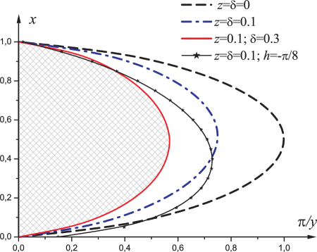
Figure 3: (Color online) The phase diagram exhibits the regions with magnetic and nonmagnetic states.

The behavior of magnetic moment at constant value of the effective impurity charge is presented in figure 2 when the parameter $y=U_{0}/\Delta$ increases. When $y$ is large but finite, magnetic solutions are still possible but as $y$ is reduced they eventually disappear.

The diagram describing the region of existence of magnetic and nonmagnetic states is presented in figure 3. The interplay of hybridization and local environment disorder produces a rich structure zero-temperature phase diagram. The region of impurity magnetic states in a disordered metal decreases in contrast to the quasi-crystalline case ($\delta=0$) [28]. This famous experimental fact for ferromagnetic alloys is discussed in various monographs, see e.g. [7].

The solvation free energy, $\Delta E$, that determines the excess free energy associated with the insertion of an impurity atom into liquid metal, was calculated for this model in our earlier work [27] that corresponds to the quasi-crystalline case. The dependence of $\Delta E$, caused by the impurity solvation in liquid metal, on Fermi level $x$, is shown in figure (4). The dotted lines correspond to the cases when the structural disorder is taken into account. The solid lines correspond to the quasi-crystalline approximation [27].

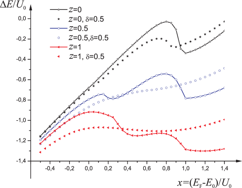
Figure 4: (Color online) The solvation free energy of impurity atom in liquid metal.

6 Conclusions

A generalized model proposed in this article permits to calculate the microscopic characteristics of impurity states in liquid metal and to analyze the effect of the structural disorder on the macroscopic properties.

Using the equation of motion method for the two-time retarded Green function and using HFA, the system of self-consistent equations for average thermodynamic occupation numbers of localized impurity level is obtained. The region of impurity magnetic states in a disordered metal decreases in contrast to the quasi-crystalline case. The contribution to the broadening of virtual impurity level at $T=0$ comes from the scattering processes on the charged impurity and from the structural disorder of the impurity environment as well. This interplay may be relevant to experimental realizations of the system ‘‘liquid metal+electronegative impurity’’ in order to study its magnetic properties.

The next possible step of exploration of the proposed model can be the study of Kondo regime taking into account the processes of exchange. In the discussed Hamiltonian (2.7), these processes are described by the following terms, $a_{\bf{k}1\sigma}^{+}\,a_{\bf{k}2\sigma^{\prime}}^{+}d_{0,\sigma^{\prime}}d_{0,\sigma}$,   $d_{0,\sigma^{\prime}}^{+}d_{0,\sigma^{\prime}}^{+}a_{\bf{k}2\sigma^{\prime}}\,a_{\bf{k}1\sigma}$,   $a_{\bf{k}1\sigma}^{+}\,d_{0,\sigma^{\prime}}^{+}a_{\bf{k}2\sigma^{\prime}}d_{0,\sigma}$, that correspond to the spin flip processes. They were not accounted for because their matrix elements are of an order of magnitude less than the Coulomb matrix elements. However, using these terms and the decoupling scheme beyond the HFA one can analyse the Kondo effect, which is important at low temperatures. This exchange interaction is more likely to increase the polarization of the band electrons rather than to enhance the formation of a magnetic moment.

Ukrainian 0 Магнiтнi стани iзольованої домiшки у невпорядкованому середовищi

Г.В. Понедiлок, М.I. Клапчук

             
Нацiональний унiверситет ’’Львiвська полiтехнiка’’, Iнститут прикладної математики
та фундаментальних наук, вул. С. Бандери, 12, 79013 Львiв, Україна

References

• [1] Anderson P., Phys. Rev., 1961, 124, 41; doi:10.1103/PhysRev.124.41.
• [2] Edwards S.F., Proc. Roy. Soc., 1962, A267, 518; doi:10.1098/rspa.1962.0116.
• [3] Roth L.M., Phys. Rev. B, 1972, 7, 4321; doi:10.1103/PhysRevB.7.4321.
• [4] Ishida Y.,Yonezawa F., Prog. Theor. Phys., 1973, 49, 731; doi:10.1143/PTP.49.731.
• [5] Kaneyoshi T., J. Phys. C: Solid State Phys., 1972, 5, 3504; doi:10.1088/0022-3719/5/24/013.
• [6] Schwartz L., Phys. Rev. B, 1973, 7, 4425; doi:10.1103/PhysRevB.7.4425.
• [7] Xandrich K., Kobe S., Amorphe Ferro- und Ferrimagnetika, Akademie-Verlag, Berlin, 1980.
• [8] Rudavskii Yu., Ponedilok G., Klapchuk M., Preprint of the Institute for Condensed Matter Physics, ICMP-02-13U, Lviv, 2002 (in Ukrainian).
• [9] Rudavskii Yu., Ponedilok G., Klapchuk M., Preprint of the Institute for Condensed Matter Physics, ICMP-02-24U, Lviv, 2003 (in Ukrainian).
• [10] Zubarev D.N., Sov. Phys. Usp., 1960, 3, 320; doi:10.1070/PU1960v003n03ABEH003275 [Usp. Fiz. Nauk, 1960, 71, 71 (in Russian)].
• [11] Luo H.G., Ying Ju., Wang S., Phys. Rev. B, 1999, 59, 9710; doi:10.1103/PhysRevB.59.9710.
• [12] Rudavskii Yu., Ponedilok G., Klapchuk M., Condens. Matter Phys., 2003, 36, 611; doi:10.5488/CMP.6.4.611.
• [13] Rudavskii Yu., Ponedilok G., Klapchuk M., J. Phys. Stud., 2005, 8, 352.
• [14] Hubbard J., Proc. R. Soc. Lond. A, 1963, 276, 238; doi:10.1098/rspa.1963.0204.
• [15] Hewson A.C., Phys. Rev., 1966, 144, 420; doi:10.1103/PhysRev.144.420.
• [16] Haldane F.D.M., Anderson P.W., Phys. Rev. B, 1976, 13, 2553; doi:10.1103/PhysRevB.13.2553.
• [17] Haldane F.D.M., Phys. Rev. B, 1977, 15, 281; doi:10.1103/PhysRevB.15.281.
• [18] Kishore R., Joshi S.K., Phys. Rev. B, 1970, 2, 1411; doi:10.1103/PhysRevB.2.1411.
• [19] Ostrovskii O.I., Grygorian V.A., Vishkariov A.F., Properties of Metallic Alloys, Moscow, Metallurgia, 1988 (in Russian).
• [20] Harrison U., Pseudopotentials in Theory of Metals, Moscow, Mir, 1968 (in Russian).
• [21] Yuhnovskii I.R., Gurskii Z.A., Quantum Statistic Theory of Disordered System, Kiev, Naukova Dumka, 1991 (in Ukrainian).
• [22] Aschkroft N., Lekner J., Phys. Rev., 1966, 145, 83; doi:10.1103/PhysRev.145.83.
• [23] Smirnow B.M., Negative Ions, Moscow, Atomizdat, 1978 (in Russian).
• [24] Golovinskii P.A., Zon B.A., Izv. An. SSSR Fiz.+, 1981, 45, 2305 (in Russian).
• [25] Cooper J.W., Martin J.B., Phys. Rev., 1962, 126, 1482; doi:10.1103/PhysRev.126.1482.
• [26] Robinson E.J., Geltman S., Phys. Rev., 1967, 153, 4; doi:10.1103/PhysRev.153.4.
• [27] Rudavskii Yu.K., Ponedilok G.V., Klapchuk M.I., Ukr. J. Phys., 2005, 50, 1308 (in Ukrainian).
• [28] Rudavskii Yu., Ponedilok G., Klapchuk M., Preprint of the Institute for Condensed Matter Physics, ICMP-06-19U, Lviv, 2006 (in Ukrainian).
\@nopatterns
Ukrainian \adddialect\l@ukrainian0 \l@ukrainian Магнiтнi стани iзольованої домiшки у невпорядкованому середовищi