Exact dynamics for optical coherent-state qubits subject to environment noise

Abstract

We study the exact dynamics of optical qubits encoded via coherent states with opposite phases which are interacting with an environment modeled as a collection of simple harmonic oscillators. Making use of a coherent-state path integral formulation, we are able to study memory effects on the dynamics of the coherent-state qubits due to strong environment coupling. We apply this formulation to examine the time evolution of a noisy quantum channel formed by two coherent-state qubits that are subject to uncorrelated local environment noises. In particular, we examine the time evolution of entanglement and maximal teleportation fidelity of the noisy quantum channel and show that at strong coupling, due to large feedback effects from the environment noise, it is possible to maintain a robust quantum channel in the long-time limit if appropriate error-correcting code is applied.

I Introduction

Classical computation and information theories have chiefly been based on encoding bit states for computing and information processing using discrete classical variables taking two values, say, 0 and 1. Quantum mechanics has opened up new possibilities for representing the bit states making use of quantum mechanical states, such as $|0\rangle$ and $|1\rangle$ along with their superpositions. This brings computational theory to a new horizon, since new algorithms have proved to be able to solve problems that are believed to be unsolvable classically Sho ; Gro . At the same time, it has also revolutionized information theory in that new communication protocols can reach unprecedented security level that is classically impossible [NC, –Bou, ].

In standard approaches to quantum computing and quantum information processing, one adopts two orthogonal basis states, denoted $|0_{L}\rangle$ and $|1_{L}\rangle$ to encode the logical states of the quantum bits (qubits), which can be two orthogonal spin states of electrons or nuclear moments, or two orthogonal polarization states of single photons NC . In recent years, however, there has been a rapid growth of interest in an alternative approach which encodes quantum information using continuous (quantum) variables cv1 ; cv2 . Since unconditional quantum operations can be achieved in this scheme, it has the merit of significantly reducing the resource overhead for quantum information processing (though with non-ideal fidelities). For optical implementations, the continuous-variable approach has the additional advantage of experimental accessibility KL . Typically, in optical implementations the quantum information is encoded using the quadrature variables (for instance, the “position” and the “momentum” operators) of the electromagnetic fields which have continuous spectra. The experimental detections of the quantum states can then be achieved using homodyne detections with high efficiency and accuracy. Moreover, various quantum optical techniques are available for quantum state manipulations necessary for gate operations.

Along with these developments, Jeong and Kim Jeon02 , and Ralph et al. Ralph03 propose to encode the logical states of qubits using two coherent states with unequal amplitudes, for example,

$$|0_{L}\rangle\mapsto|\alpha\rangle\qquad\mbox{and}\qquad|1_{L}\rangle\mapsto|\beta\rangle\,,$$ (1)

where $|\alpha\rangle$, $|\beta\rangle$ are coherent states with (complex) amplitudes $\alpha$, $\beta$, respectively, for an optical mode. The coherent states are defined as Walls

$$|\alpha\rangle\equiv e^{\alpha\hat{a}^{\dagger}-\alpha^{*}\hat{a}}|0\rangle=e^{-\frac{|\alpha|^{2}}{2}}\sum_{n=0}^{\infty}\frac{\alpha^{n}}{\sqrt{n!}}|n\rangle\,,$$ (2)

where $\hat{a}$ is the annihilation operator for the optical mode, and $|n\rangle$ the number state with $n$ photons, so that $|0\rangle$ represents the vacuum state. Although coherent states with finite amplitudes are not exactly orthogonal to each other (thus causing errors in quantum computing tasks and reduced fidelity in quantum information processing), the coherent-state approach has several advantages. Among them, due to the continuous spectra of coherent states, this scheme is thus a “hybrid” of the discrete-variable and the continuous-variable approaches. It therefore inherits merits from both approaches, so that unconditional single-qubit gate operations can be implemented via offline resource states, linear optical networks, photon counting, and classical feedforward Ralph03 . In particular, it has been shown that based on this scheme efficient quantum gates can be implemented Jeong and fault-tolerant quantum computation can be achieved with experimentally accessible amplitudes for the coherent states Lund08 . At the same time, quantum error-correcting codes have also been developed for the coherent-state logic [Glancy, –Wick13, ]. Experimentally, the resource states for this scheme (the “cat states”) can be generated using photon subtractions [Ourj07, –Ourj09, ], making the scheme a promising candidate for realistic quantum computing and quantum information processing.

As with other realizations for quantum computing and quantum information processing, coherent-state qubits are inevitably exposed to environment noises. For instance, when an optical coherent-state passes through an optical element (e.g., a beam splitter) that is part of a quantum gate, photon loss can occur due to finite absorption coefficient of the element. In any realistic analysis, it is therefore essential to take into account such effects. Earlier works in this regard have primarily focused on the limit of weak qubit-environment interactions and/or negligible environment-noise coherence time compared with the time scale for the qubit dynamics, so that the Born-Markov approximation can be invoked Jeong ; Glancy ; Mun10 ; Wick10 . In recent years, however, it has been recognized that such considerations are not satisfactory for most realistic conditions. In particular, for full scale quantum computing it may be necessary to integrate optical systems with, for instance, solid-state systems obrien . At the interface between these systems, more complicated decoherence mechanisms may arise compared with those in all-optical settings. The study of non-Markovian dynamics for open quantum systems has therefore become a key issue [Wolf, –LoF, ]. In the present work, we aim to study the exact open-system dynamics for coherent-state qubits making use of a formulation based on coherent-state path integrals developed by Zhang and collaborators [An, –WM12, ]. This formulation will allow us to study non-perturbatively the dynamics of coherent-state qubits in the presence of strong environment noise. In particular, we will consider a noisy quantum channel, which consists of two entangled qubits that are interacting with their local environments, and examine the time evolution of its entanglement and teleportation fidelity. Surprisingly, we find that at strong coupling, due to feedback effects from the environment noise, it is possible to preserve at long time the entanglement of the two qubits and achieve better-than-classical teleportation fidelity if an appropriate error-correcting code is applied. This demonstrates that it is feasible to establish a robust coherent-state quantum channel even in the presence of environment noise.

We will start in Sec. II by introducing a model for dissipation which allows exact solutions via coherent-state path integral formulation. We will then examine the exact dynamics of a single coherent-state qubit subject to such environment noise. In Sec. III the analysis will be extended to two entangled qubits that constitute a quantum channel. We will look into the time evolution of the entanglement and teleportation fidelity of the quantum channel in the presence of dissipation. Then in Sec. IV we will study how error-correcting codes can help recover the entanglement and teleportation fidelity of the pair of coherent-state qubits at long time. Finally, in Sec. V we summarize our findings and offer brief discussions over related issues.

II Formulation

To study decoherence of the coherent-state qubits, let us suppose the optical mode (henceforth the “CS mode”) adopted for coherent-state encoding undergoes dissipation due to photon loss to its environment. This dissipation has previously been modeled with a beam splitter which deflects photons from the CS mode into an environment mode Glancy ; Mun10 ; Wick10 . Since the dissipation is characterized solely by the transmissivity of the beam splitter, it has no dynamics in this simple model Wick10 . Although one could phenomenologically ascribe an exponentially decaying time-dependence to the transmissivity, the dynamics would invariably be Markovian for which no memory effect from the environment coupling can arise Mun10 . In order to overcome this difficulty, let us consider a generic model in which the CS mode interacts with an environment that consists of a collection of simple harmonic oscillator modes. The total Hamiltonian thus reads (we set $\hbar=1$ throughout) loui

$$H=\omega_{0}\hat{a}^{\dagger}\hat{a}+\sum_{k}\omega_{k}\hat{b}_{k}^{\dagger}\hat{b}_{k}+\sum_{k}\left(V_{k}\hat{a}^{\dagger}\hat{b}_{k}+V_{k}^{*}\hat{b}_{k}^{\dagger}\hat{a}\right)\,,$$ (3)

where $\omega_{0}$ is the CS mode frequency and $\hat{a}$ the corresponding annihilation operator, $\hat{b}_{k}$ is the annihilation operator for the $k$-th environment mode with frequency $\omega_{k}$, which is coupled to the CS mode with amplitude $V_{k}$. In this model, the CS mode exchanges energy with each environment mode through a beam-splitter interaction Hamiltonian Weiss . These environment modes can correspond to, for instance, phonon modes in a solid or other photon modes. The Hamiltonian (3) therefore provides a generic model for photon loss which may be relevant for interfacing between optical and solid-state systems, for instance in integrated quantum optical circuits obrien . In the limit of weak coupling, it reduces to a beam-splitter model with transmissivity that decays exponentially with time (see later in this section) Jeong . For general coupling, this generic model can exhibit richer dynamics than that of the beam-splitter model, as we will see in the following Xion . In particular, memory effects due to environment feedback at strong coupling can lead to novel dynamics for the coherent-state qubits.

In the context of damped harmonic oscillators, the Hamiltonian (3) has previously been studied under the Born-Markov approximation loui ; barnett . In order to examine feedback effects from the environment noise, it is necessary to go beyond this limit. This has been achieved by Zhang and coworkers [An, –WM12, ] using coherent-state path integrals applied to the Feynman-Vernon influence functional formalism An ; FV . In essence, one starts from the time evolution of the density matrix $\rho_{tot}$ for the total system (including the CS mode and the environment)

$$\rho_{tot}(t)=e^{-iH(t-t_{0})}\rho_{tot}(t_{0})e^{+iH(t-t_{0})}\,,$$ (4)

where $t_{0}$ is the initial time and the Hamiltonian $H$ is given by (3). In the coherent-state representation, one has the completeness relation Walls ; note

$$\int\frac{d^{2}\alpha}{\pi}|\alpha\rangle\langle\alpha|=\hat{I}\,,$$ (5)

where the integral extends over the entire complex $\alpha$-plane and $d^{2}\alpha\equiv d\,\mbox{Re}\{\alpha\}\,d\,\mbox{Im}\{\alpha\}$ with Re, Im indicating the real and imaginary parts, respectively; the coherent state $|\alpha\rangle$ are defined earlier in (2), and $\hat{I}$ is the identity operator. Utilizing (5), one can express (4) in terms of coherent-state basis for the CS mode and the environment modes. By integrating out all environment degrees of freedom, one can then arrive at an effective equation for the time evolution of the CS mode which is encoded with the full environment effects.

Let us suppose the CS mode and the environment modes are completely decoupled initially, and the environment starts off in the vacuum state at zero temperature. The initial total density matrix is thus

$$\rho_{tot}(t_{0})=\rho(t_{0})\otimes|0_{E}\rangle\langle 0_{E}|\,,$$ (6)

where $\rho(t_{0})$ is the initial density matrix for the CS mode and $|0_{E}\rangle$ denotes vacuum state for the environment modes. Using (6) in (4) and tracing out all environment modes in the coherent-state basis, one can derive a path-integral representation for the time evolution of the reduced density matrix for the CS mode An . Expressing the reduced density matrix for the CS mode at time $t$

$$\rho(t)=\int\frac{d^{2}\alpha_{f}}{\pi}\int\frac{d^{2}\alpha_{f}^{\prime}}{\pi}\rho(\alpha_{f}^{*},\alpha_{f}^{\prime};t)|\alpha_{f}\rangle\langle\alpha_{f}^{\prime}|\,,$$ (7)

where $\alpha^{*}$ denotes the complex conjugate of $\alpha$ and $\rho(\alpha_{f}^{*},\alpha_{f}^{\prime};t)\equiv\langle\alpha_{f}|\rho(t)|\alpha_{f}^{\prime}\rangle$, one finds in the influence functional formulation the time evolution for the matrix elements of the reduced density matrix

$$\rho(\alpha_{f}^{*},\alpha_{f}^{\prime};t)=\int\frac{d^{2}\alpha_{i}}{\pi}\int\frac{d^{2}\alpha_{i}^{\prime}}{\pi}\rho(\alpha_{i}^{*},\alpha_{i}^{\prime};t_{0}){\cal K}(\alpha_{i},\alpha_{i}^{\prime},\alpha_{f},\alpha_{f}^{\prime};t,t_{0})\,,$$ (8)

where the kernel ${\cal K}$ now incorporates the entire environment effects in the Hamiltonian (3) An ; FV . At zero temperature the kernel is given by Xion

$${\cal K}(\alpha_{i},\alpha_{i}^{\prime},\alpha_{f},\alpha_{f}^{\prime};t,t_{0})=A(t)\exp\left\{\alpha_{f}^{*}u(t)\alpha_{i}+\alpha_{i}^{\prime*}B(t)\alpha_{i}+\alpha_{i}^{\prime*}u^{*}(t)\alpha_{f}^{\prime}\right\}$$ (9)

with note

$$A(t)=e^{-\frac{1}{2}(|\alpha_{i}|^{2}+|\alpha_{i}^{\prime}|^{2}+|\alpha_{f}|^{2}+|\alpha_{f}^{\prime}|^{2})}\,,\quad B(t)=1-|u(t)|^{2}\,.$$ (10)

Here $u(t)$ follows the equation of motion

$$\frac{d}{dt}u(t)+i\omega_{0}u(t)+\int_{t_{0}}^{t}d\tau g(t-\tau)u(\tau)=0\,$$ (11)

subject to the initial condition $u(t_{0})=1$. As we will notice in the following, $u(t)$ plays an essential role in the dynamics of coherent-state qubits. In (11) we have introduced the noise correlation function

$$g(t)=\int_{0}^{\infty}\frac{d\omega}{2\pi}J(\omega)e^{-i\omega t}\,,$$ (12)

where $J(\omega)$ is the spectral function for the CS mode-environment coupling in (3)

$$J(\omega)=\sum_{k}|V_{k}|^{2}\delta(\omega-\omega_{k})\,.$$ (13)

Namely it is the density of the environment modes weighted with the modulus square of the coupling amplitude. For explicit calculations of the problem, one must have an explicit expression for the spectral function. We will defer such calculations to later and focus for the moment on establishing general formulations for the problems that will concern us.

Let us now apply the formulation above to study the decoherence dynamics of a single coherent-state qubit. In the coherent-state encoding, the initial density matrix for a single qubit has the general form

$$\rho(t_{0})=\sum_{m,n=1}^{2}c_{mn}|\alpha_{m}\rangle\langle\alpha_{n}|\,,$$ (14)

where $c_{mn}$ are time-independent coefficients and $\alpha_{m,n}$ take values at the encoding amplitudes. Throughout this work we will adopt coherent states with opposite phases as the encoding basis. Therefore, for instance, with the encoding basis $|\pm\alpha_{0}\rangle$, one would have in the equation above $\alpha_{1,2}=\pm\alpha_{0}$. From (14), it is clear that the time evolution of the density matrix is entirely delegated to the elements $|\alpha_{m}\rangle\langle\alpha_{n}|$. Our first task is therefore to work out the time evolution of such an element.

Let us consider an arbitrary element $\sigma(t_{0})\equiv|\alpha\rangle\langle\beta|$. In the coherent-state representation, its matrix elements are

$$\sigma(\alpha_{i}^{*},\alpha_{i}^{\prime};t_{0}) = \langle\alpha_{i}|\Big{(}|\alpha\rangle\langle\beta|\Big{)}|\alpha_{i}^{\prime}\rangle=\langle\alpha_{i}|\alpha\rangle\langle\beta|\alpha_{i}^{\prime}\rangle$$ (15)

$$= e^{-\frac{1}{2}\left(|\alpha_{i}|^{2}+|\alpha|^{2}-2\alpha_{i}^{*}\alpha\right)}e^{-\frac{1}{2}\left(|\beta|^{2}+|\alpha_{i}^{\prime}|^{2}-2\beta^{*}\alpha_{i}^{\prime}\right)}\,.$$

The time evolution of the matrix element (15) can be found using (8), with $\sigma$ here in place of the reduced density matrix $\rho$. The integrals over $\alpha_{i}$ and $\alpha_{i}^{\prime}$ are Gaussian integrals which can be dealt with easily and yield

$$\sigma(\alpha_{f}^{*},\alpha_{f}^{\prime};t) = e^{-\frac{1}{2}\left(|\alpha|^{2}+|\beta|^{2}\right)+\alpha(1-|u(t)|^{2})\beta^{*}}$$ (16)

$$\times e^{-\frac{1}{2}\left(|\alpha_{f}|^{2}+|\alpha_{f}^{\prime}|^{2}\right)+\alpha u(t)\alpha_{f}^{*}+\beta^{*}u^{*}(t)\alpha_{f}^{\prime}}\,.$$

Substituting (16) back into (7) and, as above, replacing $\rho$ with $\sigma$, one can carry out the integrals over $\alpha_{f}$ and $\alpha_{f}^{\prime}$, and arrive at the following prescription for the exact dynamics for the element $|\alpha\rangle\langle\beta|$ in the presence of environment noise

$$|\alpha\rangle\langle\beta|\longrightarrow e^{-\frac{1-|u(t)|^{2}}{2}(|\alpha|^{2}+|\beta|^{2}-2\alpha\beta^{*})}|\alpha u(t)\rangle\langle\beta u(t)|\,,$$ (17)

where the arrow indicates time evolution. Equipped with (17), we are now able to find the exact time evolution for a coherent-state qubit with any initial density matrix. We will therefore refer to this result repeatedly in the rest of this paper.

As an example, let us consider a coherent-state qubit initially in the “cat state” in the basis $\{|\pm\alpha_{0}\rangle\}$

$$|Q\rangle=\frac{1}{\sqrt{N}}\left(c_{1}|\alpha_{0}\rangle+c_{2}|-\alpha_{0}\rangle\right)\,,$$ (18)

where $|c_{1}|^{2}+|c_{2}|^{2}=1$ and $N=1+e^{-2|\alpha_{0}|^{2}}(c_{1}^{*}c_{2}+c_{1}c_{2}^{*})$ is a normalization factor (note that it depends on $c_{1}$, $c_{2}$ and thus cannot be absorbed into them). Following the prescription (17), the time evolution of the state (18) subject to dissipations due to the Hamiltonian (3) can be obtained easily

$$\rho(t) = \frac{1}{N}[\,|c_{1}|^{2}|\alpha_{t}\rangle\langle\alpha_{t}|+|c_{2}|^{2}|-\alpha_{t}\rangle\langle-\alpha_{t}|$$ (19)

$$+ e^{-2(|\alpha_{0}|^{2}-|\alpha_{t}|^{2})}\left(c_{1}c_{2}^{*}|\alpha_{t}\rangle\langle-\alpha_{t}|+c_{1}^{*}c_{2}|-\alpha_{t}\rangle\langle\alpha_{t}|\right)\,]\,.$$

Note that, for brevity here we have denoted

$$\alpha_{t}\equiv\alpha_{0}u(t)\,,$$ (20)

which will also be used in the rest of this paper. Since the absolute value of $u(t)$ turns out to be always less than 1 for $t>t_{0}$, the environment noise thus causes amplitude reduction in the coherent-state qubit note4 and induces phase damping through the off-diagonal elements of the density matrix. In the limit of weak coupling, or when the coupling has a broad spectrum, the spectral function $J(\omega)$ would have weak frequency dependence, so that the noise correlation function (12) becomes a sharp function in time. Taking $t_{0}=0$, one can find from (11) in this limit barnett ; Xion

$$u(t)\simeq e^{-\left(i\omega_{0}^{\prime}+\frac{J(\omega_{0})}{2}\right)t}$$ (21)

with $\omega_{0}^{\prime}=\omega_{0}+{\cal P}\int_{0}^{\infty}d\omega\frac{J(\omega)}{\omega-\omega_{0}}$, where $\cal P$ denotes principal value of the integral. Therefore, in this limit the coherent-state amplitude decays exponentially with time and Eq. (19) reduces to the Markovian result obtained in Ref. Jeong, . For general coupling strength, however, $u(t)$ can have quite different time dependence and novel qubit dynamics can emerge, as we will soon discover.

It is interesting to note that the result (19) can be expressed in the form of an operator sum Wick10 ; Kraus

$$\rho(t)=(1-p_{e})|Q_{t}\rangle\langle Q_{t}|+p_{e}\hat{Z}|Q_{t}\rangle\langle Q_{t}|\hat{Z}^{\dagger}\,,$$ (22)

where $p_{e}\equiv(1-e^{-2(|\alpha_{0}|^{2}-|\alpha_{t}|^{2})})/2$ and $|Q_{t}\rangle$ is the state $|Q\rangle$ of (18) with $|\pm\alpha_{0}\rangle$ replaced by $|\pm\alpha_{t}\rangle$ (the factor $N$ remains the same; thus $|Q_{t}\rangle$ is not normalized), and we have introduced the “Pauli-$Z$” operator $\hat{Z}$ such that

$$\hat{Z}|\pm\alpha_{t}\rangle=\pm|\pm\alpha_{t}\rangle\,.$$ (23)

Note that here $\hat{Z}$ is neither Hermitian nor unitary note2 . It follows immediately from (22) that the dynamical map induced by the environment noise consists of two parts: the mapping of $|Q\rangle$ to $|Q_{t}\rangle$ (or damping of $\alpha_{0}$ to $\alpha_{t}$) and the random application of the Pauli-$Z$ operator. We therefore recognize that the decoherence due to the interaction Hamiltonian in (3) has a two-fold effect over the coherent-state qubit Glancy :

(a) reduction of the coherent-state amplitude through $$u(t)$$,

(b) generation of random phase-errors with probability $$p_{e}$$. (24)

As we shall find out, this is a crucial observation, since it suggests the appropriate error-correcting code to be employed when one wishes to recover the coherence of the qubit Wick10 , which we shall discuss in Sec. IV.

III Exact dynamics of two qubits

Let us now turn to the problem of two coherent-state qubits under the influence of environment noise. In this case, it would be interesting to look into a quantum channel formed by two entangled qubits and examine how its quality degrades under the action of environment noise. For this purpose, let us consider an initial state which has been of experimental interest (the cluster-type entangled coherent state) Mun10 ; ct

$$|C\rangle=\frac{1}{\sqrt{M}}\left(|\alpha_{0},\alpha_{0}\rangle-z|\alpha_{0},-\alpha_{0}\rangle-z|-\alpha_{0},\alpha_{0}\rangle-z^{2}|-\alpha_{0},-\alpha_{0}\rangle\right)\,,$$ (25)

where $M=4(1+e^{-4|\alpha_{0}|^{2}})$, $z=-i$ (which is kept implicit here for later convenience), and $|\alpha_{0},\alpha_{0}\rangle=|\alpha_{0}\rangle\otimes|\alpha_{0}\rangle$ etc denote coherent states of the two CS modes in question. Here, again, each qubit is encoded with the $\{|\pm\alpha_{0}\rangle\}$ basis states. When the two CS modes are subject to independent dissipations induced by the Hamiltonian (3) with the same spectral function, the time evolution of the CS modes can then be found in accordance with the single qubit case. Namely, with each mode following the prescription (17), we have the following for the time evolution of any element in a two-qubit density matrix

$$|\alpha,\alpha^{\prime}\rangle\langle\beta,\beta^{\prime}|=|\alpha\rangle\langle\beta|\otimes|\alpha^{\prime}\rangle\langle\beta^{\prime}|$$

$$\rightarrow e^{-\frac{1-|u(t)|^{2}}{2}(|\alpha|^{2}+|\alpha^{\prime}|^{2}+|\beta|^{2}+|\beta^{\prime}|^{2}-2(\alpha\beta^{*}+\alpha^{\prime}\beta^{\prime*}))}|\alpha u(t),\alpha^{\prime}u(t)\rangle\langle\beta u(t),\beta^{\prime}u(t)|\,.$$ (26)

It is then easy to work out the exact dynamics for the initial state (25). Its density matrix at any time $t>t_{0}$ is found to be

$$\rho(t)=\frac{1}{M}[\,|\alpha_{t},\alpha_{t}\rangle\langle\alpha_{t},\alpha_{t}|-ic|\alpha_{t},\alpha_{t}\rangle\langle\alpha_{t},-\alpha_{t}|-ic|\alpha_{t},\alpha_{t}\rangle\langle-\alpha_{t},\alpha_{t}|+c^{2}|\alpha_{t},\alpha_{t}\rangle\langle-\alpha_{t},-\alpha_{t}|$$

$$+ic|\alpha_{t},-\alpha_{t}\rangle\langle\alpha_{t},\alpha_{t}|+|\alpha_{t},-\alpha_{t}\rangle\langle\alpha_{t},-\alpha_{t}|+c^{2}|\alpha_{t},-\alpha_{t}\rangle\langle-\alpha_{t},\alpha_{t}|+ic|\alpha_{t},-\alpha_{t}\rangle\langle-\alpha_{t},-\alpha_{t}|$$

$$+ic|-\alpha_{t},\alpha_{t}\rangle\langle\alpha_{t},\alpha_{t}|+c^{2}|-\alpha_{t},\alpha_{t}\rangle\langle\alpha_{t},-\alpha_{t}|+|-\alpha_{t},\alpha_{t}\rangle\langle-\alpha_{t},\alpha_{t}|+ic|-\alpha_{t},\alpha_{t}\rangle\langle-\alpha_{t},-\alpha_{t}|$$

$$+c^{2}|-\alpha_{t},-\alpha_{t}\rangle\langle\alpha_{t},\alpha_{t}|-ic|-\alpha_{t},-\alpha_{t}\rangle\langle\alpha_{t},-\alpha_{t}|-ic|-\alpha_{t},-\alpha_{t}\rangle\langle-\alpha_{t},\alpha_{t}|+|-\alpha_{t},-\alpha_{t}\rangle\langle-\alpha_{t},-\alpha_{t}|\,]\,.$$

(27)

Here $M$ is the same as in (25) and we have denoted $c\equiv 1-2p_{e}=\exp\{-2(|\alpha_{0}|^{2}-|\alpha_{t}|^{2})\}$. Note that this result can also be obtained using the operator sum formulation by extending (22) to two CS modes subject to independent, identical dissipations wu12 . Equation (27) thus describes the exact time evolution of a noisy quantum channel initially in the state (25) with each CS mode under the action of the Hamiltonian (3).

To examine the quality of the noisy quantum channel, we shall study the change of its entanglement property and teleportation ability with time. To this end, we shall calculate the time evolution of the concurrence Woot and maximal teleportation fidelity Horod for the density matrix (27). For bipartite two-state systems, the concurrence for a density matrix $\rho$ is defined as

$$C\equiv\max\{0,\sqrt{\lambda_{1}}-\sqrt{\lambda_{2}}-\sqrt{\lambda_{3}}-\sqrt{\lambda_{4}}\}\,,$$ (28)

where $\lambda_{i}$ are eigenvalues of $\rho(\hat{Y}_{1}\otimes\hat{Y}_{2})\rho^{*}(\hat{Y}_{1}\otimes\hat{Y}_{2})$ with $\lambda_{1}$ being the largest one. Here $\hat{Y}_{j}$ are Pauli-$Y$ operators for sub-system $j$ and $\rho^{*}$ is the complex conjugate of the density matrix $\rho$ Woot . To find the concurrence for $\rho(t)$ of (27), it is thus necessary to have first a matrix representation for the density matrix with respect to an orthonormal basis for the restricted two-mode space spanned by $\{|\pm\alpha_{t}\rangle\otimes|\pm\alpha_{t}\rangle\}$. Let us consider the following “even” and “odd” states

$$|e\rangle=\frac{1}{\sqrt{N_{e}}}\left(|\alpha_{t}\rangle+|-\alpha_{t}\rangle\right)\quad\mbox{and}\quad|o\rangle=\frac{1}{\sqrt{N_{o}}}\left(|\alpha_{t}\rangle-|-\alpha_{t}\rangle\right)\,,$$ (29)

where $N_{e,o}=2(1\pm e^{-2|\alpha_{t}|^{2}})$ are normalization factors. One can easily check using (2) that $|e\rangle$ and $|o\rangle$ consist of number states with, respectively, even and odd numbers of photons, and hence are orthogonal to each other. We can therefore employ the basis set $\{|ee\rangle,|eo\rangle,|oe\rangle,|oo\rangle\}$ for the two CS modes and arrive at the following matrix representations for the original basis states

$$|\alpha_{t},\pm\alpha_{t}\rangle=\left(\begin{array}[]{c}a^{2}\\ \pm ab\\ ab\\ \pm b^{2}\\ \end{array}\right)\,,\qquad|-\alpha_{t},\pm\alpha_{t}\rangle=\left(\begin{array}[]{c}a^{2}\\ \pm ab\\ -ab\\ \mp b^{2}\\ \end{array}\right)\,.$$ (38)

Here we have denoted

$$a=\sqrt{\frac{1+e^{-2|\alpha_{t}|^{2}}}{2}}\quad\mbox{and}\quad b=\sqrt{\frac{1-e^{-2|\alpha_{t}|^{2}}}{2}}\,.$$ (39)

Using (38) in (27), we arrive at the matrix representation for the density matrix in the basis $\{|ee\rangle,|eo\rangle,|oe\rangle,|oo\rangle\}$

$$\rho(t)=\frac{4}{M}\left(\begin{array}[]{cccc}a^{4}(1+c^{2})&0&0&2ica^{2}b^{2}\\ 0&a^{2}b^{2}(1-c^{2})&0&0\\ 0&0&a^{2}b^{2}(1-c^{2})&0\\ -2ica^{2}b^{2}&0&0&b^{4}(1+c^{2})\\ \end{array}\right)\,.$$ (44)

We note that the density matrix takes an “X-form” YE_X . Its concurrence can thus be found relatively easily. We get

$$C=\frac{2a^{2}b^{2}}{1+e^{-4|\alpha_{0}|^{2}}}\max\{0,c^{2}+2c-1\}\,.$$ (45)

The maximal teleportation fidelity (henceforth “teleportation fidelity” for short) for a quantum channel with density matrix $\rho$ is defined through its fully entangled fraction

$$f_{\rm max}\equiv\max_{|\psi\rangle}\langle\psi|\rho|\psi\rangle\,,$$ (46)

where the maximum is taken over all possible maximally entangled states $|\psi\rangle$. For two-state systems, the teleportation fidelity is then given by Horod

$$F=\frac{2f_{\rm max}+1}{3}\,.$$ (47)

To find the fully entangled fraction for the noisy channel (27), one can first recast the density matrix in terms of the following orthonormal basis set

$$|\phi_{1}\rangle \equiv |\Phi^{+}\rangle=\frac{1}{\sqrt{2}}\left(|ee\rangle+|oo\rangle\right)\,,$$

$$|\phi_{2}\rangle \equiv i|\Phi^{-}\rangle=\frac{i}{\sqrt{2}}\left(|ee\rangle-|oo\rangle\right)\,,$$

$$|\phi_{3}\rangle \equiv i|\Psi^{+}\rangle=\frac{i}{\sqrt{2}}\left(|eo\rangle+|oe\rangle\right)\,,$$

$$|\phi_{4}\rangle \equiv |\Psi^{-}\rangle=\frac{1}{\sqrt{2}}\left(|eo\rangle-|oe\rangle\right)\,,$$ (48)

where $|\Phi^{\pm}\rangle$, $|\Psi^{\pm}\rangle$ are the usual Bell states in the even-odd basis. The fully entangled fraction $f_{\rm max}$ then corresponds to the largest eigenvalue for the real part of the transformed density matrix bennett . This calculation leads to

$$f_{\rm max}=\frac{1}{2(1+e^{-4|\alpha_{0}|^{2}})}(c^{2}-2a^{2}b^{2}(1-c)^{2}+1)\,.$$ (49)

Because here each qubit is restricted to a two-dimensional state space, the teleportation fidelity for the noisy channel (27) can thus be obtained by substituting (49) back into (47).

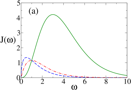
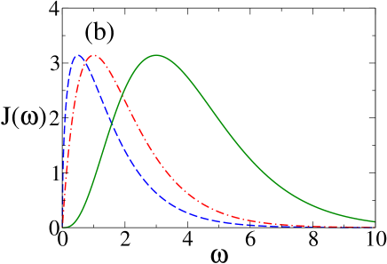
Figure 1: Spectral function $J(\omega)$ for $\eta_{0}=0.5$ (a) without scaling (i.e. $\eta_{s}=\eta_{0}$ in (50)) and (b) with scaling (i.e. with $\eta_{s}$ given by (51)) for sub-Ohmic ($s=1/2\,$; blue dashed curves), Ohmic ($s=1\,$; red dot-dashed curves), and super-Ohmic ($s=3\,$; green solid curves) cases. Here the horizontal axes are plotted in units of $\omega_{c}$, which is taken to be 1 in all plots throughout this paper.

We shall now proceed with explicit calculations for noise models for the results above. This requires a specific form for the spectral function $J(\omega)$. Here we will consider the following form of a power law with an exponential cutoff Weiss

$$J(\omega)=2\pi\eta_{s}\omega\left(\frac{\omega}{\omega_{c}}\right)^{s-1}\exp\left(-\frac{\omega}{\omega_{c}}\right)\,,$$ (50)

where (cf. Ref. Weiss, )

$$\eta_{s}=\eta_{0}\left(\frac{e}{s}\right)^{s}\,.$$ (51)

Here $\eta_{0}$ is the coupling strength and $\omega_{c}$ the cutoff frequency, which is much larger than any other frequency scales in the problem. It is common to categorize the spectral function (50) into three classes according to the power $s$ of the frequency variable $\omega$: the sub-Ohmic ($0<s<1$), Ohmic ($s=1$), and super Ohmic ($s>1$) ones Weiss . Note that unlike earlier literatures, here we have defined $\eta_{s}$ in the form (51) so that for the same $\eta_{0}$ and $\omega_{c}$, the spectral function (50) would have the same peak height $2\pi\eta_{0}\omega_{c}$ for all $s>0$; Figure 1 illustrates a comparison for $J(\omega)$ without scaling and with scaling. This would make the meaning of “coupling strength” less ambiguous when one compares results for $J(\omega)$ with different power $s$. This is because for given $s$ the peak position of $J(\omega)$ occurs at $\omega=s\omega_{c}$, its coupling is therefore “detuned” by $s\omega_{c}-\omega_{0}$ from the CS mode frequency $\omega_{0}$. Now that $J(\omega)$ for different $s$ have the same peak height (for the same $\eta_{0}$ and $\omega_{c}$), by comparing the “detunning”, one can have a clear picture as to which power $s$ would generate stronger coupling for the CS mode.

For the spectral function (50), it is not possible to obtain analytic solution for $u(t)$ from the equation of motion (11). Using techniques of Laplace transformation, however, one can express $u(t)$ as Bromwich integrals involving special functions (such as exponential integrals and error functions). Besides contribution from contours around branch-cut for the integrand, depending on the coupling strength $\eta_{0}$, the integral can also receive contribution from poles of the integrand. When the pole contribution exists, $u(t)$ would tend to non-zero steady value at long time WM12 . We relegate details of these calculations to Appendix A. Figure 2 illustrates our results for $|u(t)|$ for the coupling strengths $\eta_{0}=0.01$ and $\eta_{0}=0.5$ for different power $s$ in the spectral function (50). Here, following Ref. Xion, we consider $s=1/2$ for sub-Ohmic coupling, and $s=3$ for super-Ohmic coupling. We note that at weak coupling ($\eta_{0}=0.01$), $|u(t)|$ decays exponentially with time, while at strong coupling ($\eta_{0}=0.5$), after a sharp drop initially it recovers gradually and eventually saturates at non-zero value at long time. The weak coupling result (Fig. 2(a)) exhibits typical Markovian dynamics note3 . For the strong coupling result (Fig. 2(b)), the sharp decay is due to the large coupling between the qubit and the environment modes, which leads to a stronger decay initially than that at weak coupling. However, feedback from the environment modes subsequently bring $|u(t)|$ back and a long-time correlation between the qubit and the environment modes is gradually established, leading to non-dissipative $|u(t)|$ evolution at long time Xion . In view of Eq. (24), this means that at strong coupling the amplitude decay of the qubit saturates in the long-time limit. A natural question thus arises: For the noisy quantum channel (27), would we have a robust, non-dissipative quantum channel at long time? Namely, would the concurrence and the teleportation fidelity of the noisy quantum channel possess, respectively, non-zero steady values and better than classical values in the long-time limit?

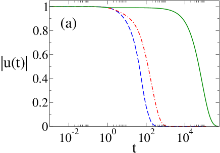
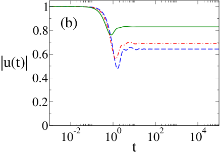
Figure 2: The absolute value of $u(t)$ for coupling strength (a) $\eta_{0}=0.01$ and (b) 0.5 for sub-Ohmic ($s=1/2\,$; blue dashed curves), Ohmic ($s=1\,$; red dot-dashed curves), and super-Ohmic ($s=3\,$; green solid curves) cases. Note that here and in all subsequent plots, we take $t_{0}=0$ and use log scale for the time axis, which is in units of $1/\omega_{c}$.

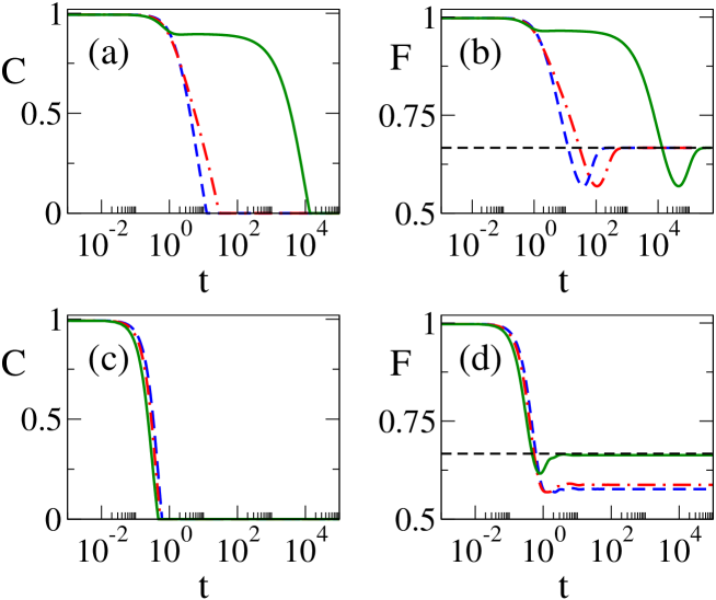
Figure 3: Concurrence $C$ and teleportation fidelity $F$ for the noisy quantum channel (27) at weak coupling ($\eta_{0}=0.01$; panels (a) and (b)) and strong coupling ($\eta_{0}=0.5$; panels (c) and (d)) for sub-Ohmic ($s=1/2\,$; blue dashed curves), Ohmic ($s=1\,$; red dot-dashed curves), and super-Ohmic ($s=3\,$; green solid curves) cases. The horizontal dashed lines in (b) and (d) indicate the classical limit $F=2/3$ for the teleportation fidelity. In all panels, the time axes are plotted in units of $1/\omega_{c}$.

To answer the questions above, we supply the numerically obtained $u(t)$ to formulas for the concurrence (45) and the teleportation fidelity (47) (by way of (49)) for the noisy quantum channel (27). For the CS mode, we shall consider an experimentally realistic initial amplitude $\alpha_{0}=1.2$ [Ourj07, –Ourj09, ] and the frequency $\omega_{0}=0.1\omega_{c}$, since the cutoff frequency $\omega_{c}$ is the largest frequency scale in the problem. The results for our calculation are demonstrated in Fig. 3 for weak ($\eta_{0}=0.01$) and strong ($\eta_{0}=0.5$) couplings with sub-Ohmic ($s=1/2$), Ohmic, and super-Ohmic ($s=3$) spectral functions. From Fig. 3(a), we see that at weak coupling the concurrence decays monotonically to zero for all three cases, with the sub-Ohmic case having the largest decay rate and the super-Ohmic one the smallest. This can be understood easily because the super-Ohmic case has the largest detunning (with its peak at $\omega=3\omega_{c}$) from the CS mode frequency ($\omega_{0}=0.1\omega_{c}$), while the sub-Ohmic case has the smallest (with peak position at $\omega=0.5\omega_{c}$). In the long-time limit, as Fig. 3(b) shows, the teleportation fidelities of all three cases drop to the classical value $2/3\simeq 0.667$ pope . Thus, as anticipated, at weak coupling the quality of the noisy channel (27) does degrade with time.

For strong coupling, despite the non-dissipative evolution of $u(t)$ at long time, we see in Figs. 3(c), (d) that the concurrence decays monotonically to zero at even faster rates than at weak coupling, and the teleportation fidelity even falls below the classical value at long time. In other words, in terms of the two figures-of-merit considered here, at strong coupling the quantum channel has a lower quality than that at weak coupling. This is surprising because the long-time correlation in $u(t)$ turns out not helpful in preserving the quantum channel at long time, in spite of the non-dissipative time evolution. Nevertheless, if one recalls from Eq. (24) that the effects of the environment noise on the qubits are in fact two-fold, it is then clear why such results emerge: The non-dissipative evolution at long time is not enough to support the quantum channel because effect (b) in (24) is still in action here. Namely, it is the random phase-errors between the two qubits that disrupt the quantum channel at strong coupling. Therefore, in order to sustain a robust quantum channel at long time, we need to take care of both effects in (24) properly. This is the task we shall now turn to.

IV Exact dynamics of two qubits with error corrections

In order to combat against effect (b) in (24) due to the environment noise, we shall resort to schemes of quantum error-corrections. Now that we have identified these errors being due to random phase-flips, it is natural to adopt phase-flip error-correcting codes Glancy ; Wick10 . In Sec. IV.1, we will therefore examine the exact dynamics of the noisy quantum channel when a phase-flip error-correcting code is applied. As a comparison, in Sec. IV.2 we will also consider an encoding scheme (the “bit-flip encoding”) that was previously proposed for constructing quantum channels using coherent-state qubits Mun10 .

IV.1 Phase-flip error correction

To correct the random phase-flip error, we shall employ a scheme proposed by Glancy et al. Glancy for coherent-state qubits. Take three-bit encoding as an example, in this scheme the signal qubit is sent at the encoding stage together with two ancilla modes in vacuum states from the sender’s side. Making use of two sets of beam splitters simulating two CNOT operations, one subsequently applies three Hadamard gates so that the qubits can be protected against phase-flip errors. Here the Hadamard gate operates in the way that (up to normalization factors) note_H

$$|\pm\alpha\rangle\xrightarrow{\text{\tiny Hadamard}}|\alpha\rangle\pm|-\alpha\rangle\,$$ (52)

with $|\pm\alpha\rangle$ the basis states for the qubit. After passing through the noisy region, the encoded qubit first passes through another three Hadamard gates for decoding and then a sequence of beam-splitters and photodetectors for syndrome detection. According to the error syndromes, one can apply corrective operations to recover the signal qubit at the receiving end. In this way, one would be able to correct one phase-flip error in the qubits NC . More errors can be corrected similarly when more encoding ancilla modes are added. In general, an $n$-bit encoding in the present scheme can correct up to $(n-1)/2$ phase-errors ($n$ must be odd number) and the probability for an error-free transmission is NC ; Glancy

$$p_{s}=\sum_{k=0}^{\frac{n-1}{2}}\left(\begin{array}[]{c}n\\ k\end{array}\right)(1-p_{e})^{n-k}p_{e}^{k}\,,$$ (55)

where $p_{e}$ is the probability for one phase-flip error in each mode. Note that when $p_{e}<1/2$, the success probability $p_{s}$ can be made arbitrarily close to 1 with sufficiently large $n$.

To incorporate the error-correcting scheme above into our calculation for the exact dynamics of the noisy quantum channel (27), we note that the probability $p_{e}$ for phase-flip errors in our calculation is given by that in (22). Thus, according to (55), with an $n$-bit error-correcting code implemented the error probability becomes $p_{e}^{\prime}=1-p_{s}$. This corresponds to changing the previously defined $c$ in (27) into

$$c^{\prime}=1-2p_{e}^{\prime}=2p_{s}-1\,.$$ (56)

The time evolution for the concurrence and the fully entangled fraction for the error-corrected noisy quantum channel can now be obtained from (45) and (49) by simply replacing $c$ with $c^{\prime}$ above.

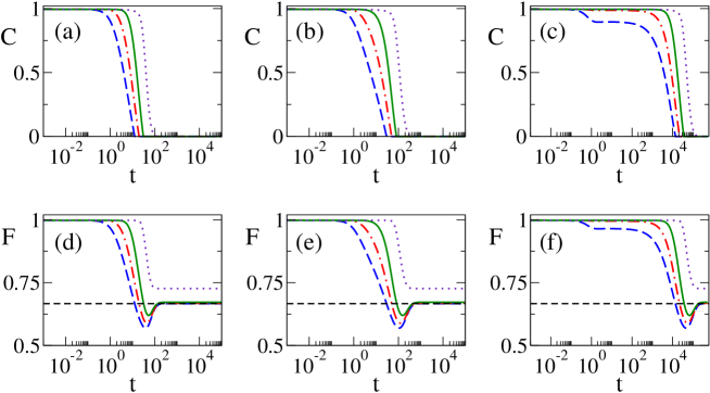
Figure 4: Concurrence $C$ and teleportation fidelity $F$ for the noisy channel at weak coupling ($\eta_{0}=0.01$) for sub-Ohmic ($s=1/2\,$; panels (a), (d)), Ohmic ($s=1\,$; panels (b), (e)), and super-Ohmic ($s=3\,$; panels (c), (f)) cases without encoding (blue dashed curves), and with phase-flip encoding using 3-bit (red dot-dashed curves), 9-bit (green solid surves), and 101-bit (purple dotted curves) codes. In each of panels (d)–(f), the horizontal dashed line signifies the classical limit $F=2/3$.

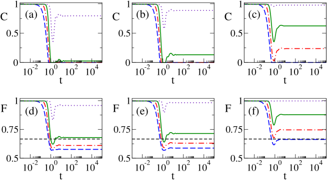
Figure 5: The same as Fig. 4 but for strong coupling ($\eta_{0}=0.5$).

The results for these calculations are shown in Fig. 4 for weak coupling ($\eta_{0}=0.01$) and Fig. 5 for strong coupling ($\eta_{0}=0.5$). One can notice immediately that at weak coupling the concurrence for all three cases have now attained longer life spans, and the teleportation fidelity can go above the classical limit after error correction is applied. These gains, however, do not seem to be very impressive as even with a 101-bit encoding, the enhancement in the teleportation fidelity is still rather limited ($F\simeq 0.727$ at large time for all three cases). Such limited gain at so high cost does not seem practical.

At strong coupling, however, the situation turns out quite different. We see from Fig. 5 that in this case, error correction can improve the concurrence and the teleportation fidelity quite significantly. For super-Ohmic coupling, with 3-bit encoding the noisy channel can maintain a non-zero concurrence ($\simeq 0.237$; see Fig. 5(c)) and a better than classical teleportation fidelity ($\simeq 0.747$; see Fig. 5(f)) at long time. With 9-bit encoding, we find that the concurrence for all three classes of spectral functions attain finite steady values and the teleportation fidelity are all raised above the classical value at long time. In the limit of large $n$ encoding (illustrated with $n=101$ here), even for the sub-Ohmic case (which would induce the strongest environment coupling due to its small detunning), the concurrence can be recovered to 0.796, and the teleportation fidelity to 0.958. Therefore, at strong coupling, the phase-flip error-correcting code can recover the noisy channel significantly and result in a robust quantum channel at long time.

To understand the results above, let us recall from (24) the two effects (a) amplitude reduction, and (b) random phase-errors due to the environment noise. As noted above, for error probability $p_{e}<1/2$ the present error-correcting code can correct phase-flip errors very efficiently. For coherent-state qubits, from (22), since $p_{e}<1/2$ always, the error-correcting code can protect the noisy channel against effect (b) very well. The difference between the weak-coupling and the strong-coupling results, therefore, is primarily due to effect (a). At weak coupling, since $|u(t)|$ decays with time monotonically to zero (see Fig. 2(a)), effect (a) persists all the way until the qubit is completely damped away. At strong coupling, however, $|u(t)|$ saturates at long time and thus effect (a) is entirely removed when this steady is reached. Therefore, for strong coupling, when the phase-flip error-correcting code is implemented, both effects from the environment noise can be accounted for and a robust quantum channel can persist at long time.

IV.2 Bit-flip encoding

In the preceding subsection, we have seen that when $u(t)$ becomes non-dissipative in the long-time limit, applying phase-flip error-correcting code can help preserve the quantum channel. As a comparison, here we shall consider a different encoding scheme for coherent-state qubits. In Ref. Mun10, , a repetition encoding was proposed for the quantum channel (25) and its performance under photon loss has been analyzed in the Markovian limit. With exact dynamics for the coherent-state qubits available, here we revisit this problem in particular for strong environment coupling when non-dissipative dynamics of $u(t)$ is present. Since this encoding scheme is identical to that in bit-flip error-correcting codes NC , in the following we will refer to it as the “bit-flip encoding” (note that no error correction is attempted in this scheme Mun10 ). Following Ref. Mun10, , an $n$-bit encoding in this scheme yields for the state (25)

$$|C_{n}\rangle=\frac{1}{\sqrt{M_{n}}} \left(|\alpha_{0}\rangle^{\otimes n}|\alpha_{0}\rangle^{\otimes n}-z^{n}|\alpha_{0}\rangle^{\otimes n}|-\alpha_{0}\rangle^{\otimes n}\right.$$ (57)

$$\left.-z^{n}|-\alpha_{0}\rangle^{\otimes n}|\alpha_{0}\rangle^{\otimes n}|-z^{2n}|-\alpha_{0}\rangle^{\otimes n}|-\alpha_{0}\rangle^{\otimes n}\right)\,,$$

where the normalization factor

$$M_{n}=\left\{\begin{array}[]{ll}4&\mbox{for even $n$,}\\ 4(1+e^{-4n|\alpha_{0}|^{2}})&\mbox{for odd $n$,}\end{array}\right.$$ (60)

and as in (25) $z=-i$; here $|\alpha\rangle^{\otimes n}\equiv|\alpha\rangle\otimes\dots\otimes|\alpha\rangle$ etc denote direct products of $n$ coherent states. Since each basis state $|\pm\alpha_{0}\rangle^{\otimes n}$ consists of $n$ independent modes, the time evolution for an element of the density matrix for the encoded state (57) at zero temperature can be generalized straightforwardly from (17)

$$|\alpha\rangle^{\otimes n}\langle\beta|^{\otimes n}\rightarrow e^{-\frac{1-|u(t)|^{2}}{2}(|\alpha|^{2}+|\beta|^{2}-2\alpha\beta^{*})n}|\alpha u(t)\rangle^{\otimes n}\langle\beta u(t)|^{\otimes n}\,$$ (61)

with $u(t)$, as before, determined from (11). The time evolution of the initial density matrix $|C_{n}\rangle\langle C_{n}|$ for (57) then follows easily from the prescription (61)

$$\rho(t)=\frac{1}{M_{n}}[\,|\alpha_{t}\rangle^{\otimes n}|\alpha_{t}\rangle^{\otimes n}\langle\alpha_{t}|^{\otimes n}\langle\alpha_{t}|^{\otimes n}-z^{*n}c^{n}|\alpha_{t}\rangle^{\otimes n}|\alpha_{t}\rangle^{\otimes n}\langle\alpha_{t}|^{\otimes n}\langle-\alpha_{t}|^{\otimes n}$$

$$-z^{*n}c^{n}|\alpha_{t}\rangle^{\otimes n}|\alpha_{t}\rangle^{\otimes n}\langle-\alpha_{t}|^{\otimes n}\langle\alpha_{t}|^{\otimes n}-z^{*2n}c^{2n}|\alpha_{t}\rangle^{\otimes n}|\alpha_{t}\rangle^{\otimes n}\langle-\alpha_{t}|^{\otimes n}\langle-\alpha_{t}|^{\otimes n}$$

$$-z^{n}c^{n}|\alpha_{t}\rangle^{\otimes n}|-\alpha_{t}\rangle^{\otimes n}\langle\alpha_{t}|^{\otimes n}\langle\alpha_{t}|^{\otimes n}+|\alpha_{t}\rangle^{\otimes n}|-\alpha_{t}\rangle^{\otimes n}\langle\alpha_{t}|^{\otimes n}\langle-\alpha_{t}|^{\otimes n}$$

$$+c^{2n}|\alpha_{t}\rangle^{\otimes n}|-\alpha_{t}\rangle^{\otimes n}\langle-\alpha_{t}|^{\otimes n}\langle\alpha_{t}|^{\otimes n}+z^{*n}c^{n}|\alpha_{t}\rangle^{\otimes n}|-\alpha_{t}\rangle^{\otimes n}\langle-\alpha_{t}|^{\otimes n}\langle-\alpha_{t}|^{\otimes n}$$

$$-z^{n}c^{n}|-\alpha_{t}\rangle^{\otimes n}|\alpha_{t}\rangle^{\otimes n}\langle\alpha_{t}|^{\otimes n}\langle\alpha_{t}|^{\otimes n}+c^{2n}|-\alpha_{t}\rangle^{\otimes n}|\alpha_{t}\rangle^{\otimes n}\langle\alpha_{t}|^{\otimes n}\langle-\alpha_{t}|^{\otimes n}$$

$$+|-\alpha_{t}\rangle^{\otimes n}|\alpha_{t}\rangle^{\otimes n}\langle-\alpha_{t}|^{\otimes n}\langle\alpha_{t}|^{\otimes n}+z^{*n}c^{n}|-\alpha_{t}\rangle^{\otimes n}|\alpha_{t}\rangle^{\otimes n}\langle-\alpha_{t}|^{\otimes n}\langle-\alpha_{t}|^{\otimes n}$$

$$-z^{2n}c^{2n}|-\alpha_{t}\rangle^{\otimes n}|-\alpha_{t}\rangle^{\otimes n}\langle\alpha_{t}|^{\otimes n}\langle\alpha_{t}|^{\otimes n}+z^{n}c^{n}|-\alpha_{t}\rangle^{\otimes n}|-\alpha_{t}\rangle^{\otimes n}\langle\alpha_{t}|^{\otimes n}\langle-\alpha_{t}|^{\otimes n}$$

$$+z^{n}c^{n}|-\alpha_{t}\rangle^{\otimes n}|-\alpha_{t}\rangle^{\otimes n}\langle-\alpha_{t}|^{\otimes n}\langle\alpha_{t}|^{\otimes n}+|-\alpha_{t}\rangle^{\otimes n}|-\alpha_{t}\rangle^{\otimes n}\langle-\alpha_{t}|^{\otimes n}\langle-\alpha_{t}|^{\otimes n}]\,,$$

(62)

where $\alpha_{t}$ is, as previously, given by (20) and $c$ the same as in (27). To find the concurrence and teleportation fidelity for the noisy channel (62), again one has to express $\rho(t)$ in terms of orthonormal basis sets. Similar to (29), we adopt the $n$-bit repetition even-odd states

$$|e_{n}\rangle=\frac{1}{\sqrt{M_{e}}}\left(|\alpha_{t}\rangle^{\otimes n}+|-\alpha_{t}\rangle^{\otimes n}\right)\quad\mbox{and}\quad|o_{n}\rangle=\frac{1}{\sqrt{M_{o}}}\left(|\alpha_{t}\rangle^{\otimes n}-|-\alpha_{t}\rangle^{\otimes n}\right)\,,$$ (63)

where $M_{e,o}=2(1\pm e^{-2n|\alpha_{t}|^{2}})$. The calculation then proceeds in close parallel with that for the non-encoded case in Sec. III, except that care must be taken over the distinction between $n$ being even or odd. In the basis $\{|e_{n}e_{n}\rangle,|e_{n}o_{n}\rangle,|o_{n}e_{n}\rangle,|o_{n}o_{n}\rangle\}$, one finds for even $n$

$$\rho(t)=\left(\begin{array}[]{cccc}a_{n}^{4}&-i^{n}a_{n}^{3}b_{n}c^{n}&-i^{n}a_{n}^{3}b_{n}c^{n}&-a_{n}^{2}b_{n}^{2}c^{2n}\\ -i^{n}a_{n}^{3}b_{n}c^{n}&a_{n}^{2}b_{n}^{2}&a_{n}^{2}b_{n}^{2}c^{2n}&i^{n}a_{n}b_{n}^{3}c^{n}\\ -i^{n}a_{n}^{3}b_{n}c^{n}&a_{n}^{2}b_{n}^{2}c^{2n}&a_{n}^{2}b_{n}^{2}&i^{n}a_{n}b_{n}^{3}c^{n}\\ -a_{n}^{2}b_{n}^{2}c^{2n}&i^{n}a_{n}b_{n}^{3}c^{n}&i^{n}a_{n}b_{n}^{3}c^{n}&b_{n}^{4}\\ \end{array}\right)\,,$$ (68)

and for odd $n$

$$\rho(t)=\frac{4}{M_{n}}\left(\begin{array}[]{cccc}a_{n}^{4}(1+c^{2n})&0&0&2i^{n}a_{n}^{2}b_{n}^{2}c^{n}\\ 0&a_{n}^{2}b_{n}^{2}(1-c^{2n})&0&0\\ 0&0&a_{n}^{2}b_{n}^{2}(1-c^{2n})&0\\ -2i^{n}a_{n}^{2}b_{n}^{2}c^{n}&0&0&b_{n}^{4}(1+c^{2n})\\ \end{array}\right)\,.$$ (73)

In both (68) and (73), we have denoted

$$a_{n}=\sqrt{\frac{1+e^{-2n|\alpha_{t}|^{2}}}{2}}\quad\mbox{and}\quad b_{n}=\sqrt{\frac{1-e^{-2n|\alpha_{t}|^{2}}}{2}}\,.$$ (74)

Accordingly, in the same manners as before, one can find for the bit-flip encoded noisy channel the concurrence

$$C=\frac{8a_{n}^{2}b_{n}^{2}}{M_{n}}\max\{0,c^{2n}+2c^{n}-1\}$$ (75)

and the fully entangled fraction

$$f_{\rm max}=\left\{\begin{array}[]{cc}\displaystyle\frac{1}{4}\left(1+4a_{n}^{2}b_{n}^{2}c^{2n}+\sqrt{(a_{n}^{2}-b_{n}^{2})^{4}+16a_{n}^{2}b_{n}^{2}c^{2n}}\right)&\mbox{for even $n$,}\\ \displaystyle\frac{1}{2(1+e^{-4n|\alpha_{0}|^{2}})}(c^{2n}-2a_{n}^{2}b_{n}^{2}(1-c^{n})^{2}+1)&\mbox{for odd $n$.}\end{array}\right.$$ (78)

As usual, using (78) in (47), one can obtain the teleportation fidelity for the encoded noisy channel.

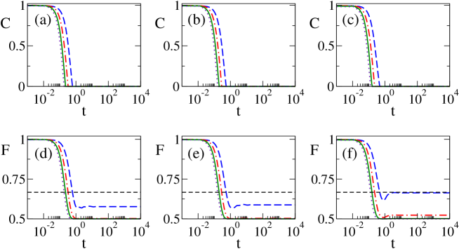
Figure 6: Concurrence $C$ and teleportation fidelity $F$ for the noisy channel at strong coupling ($\eta_{0}=0.5$) for sub-Ohmic ($s=1/2\,$; panels (a), (d)), Ohmic ($s=1\,$; panels (b), (e)), and super-Ohmic ($s=3\,$; panels (c), (f)) cases without encoding (blue dashed curves), and with bit-flip encoding using 3-bit (red dot-dashed curves), 6-bit (green solid curves), and 9-bit (purple dotted curves) codes. As in previous figures, the horizontal dashed lines in (d)–(f) indicate the classical limit $F=2/3$.

Figure 6 illustrates our results for the above calculations with the CS mode frequency $\omega_{0}=0.1\omega_{c}$ and initial amplitude $\alpha_{0}=1.2$ at strong coupling ($\eta_{0}=0.5$). Surprisingly, we find that the bit-flip encoding turns out to further degrade the quantum channel. With increasing bit redundancy in the encoding, the concurrence tends to have shorter life spans and the teleportation fidelity drops further below the classical value, despite the non-decaying $u(t)$ at long time. The bit-flip encoding here thus not only would not help recover the quantum channel, but would actually further disrupt it.

In order to see the reason for the deterioration caused by bit-flip encoding, let us apply this encoding to the cat state (18). This yields

$$|Q_{n}\rangle=\frac{1}{\sqrt{N_{n}}}\left(c_{1}|\alpha_{0}\rangle^{\otimes n}+c_{2}|-\alpha_{0}\rangle^{\otimes n}\right)\,,$$ (79)

where $N_{n}=1+e^{-2n|\alpha_{0}|^{2}}(c_{1}^{*}c_{2}+c_{1}c_{2}^{*})$. Using the prescription (61) for the time evolution of the density matrix $|Q_{n}\rangle\langle Q_{n}|$ and expressing the result as an operator sum similar to (22), one finds the phase-error probability after the bit-flip encoding becomes

$$p_{e}^{(n)}=\frac{1}{2}\left(1-e^{-2n(|\alpha_{0}|^{2}-|\alpha_{t}|^{2})}\right)\,.$$ (80)

It is then clear that with increasing bit redundancy $n$ in the encoding, the phase error actually increases. In other words, the bit-flip encoding would in fact enhance effect (b) in (24) for coherent-state qubits. Therefore, instead of reducing environment noises, the bit-flip encoding induces additional sources for phase errors, which further corrupt the noisy channel.

V Conclusions and Discussions

In summary, we have studied the exact dynamics of optical coherent-state qubits when they are exposed to environment noises. The environment is modeled with a collection of simple harmonic oscillators which interact with the qubit by exchanging energies. Making use of a coherent-state path integral formulation for this model An ; Xion , we are able to study non-perturbatively feedback effects on the qubit dynamics due to strong environment coupling. In particular, we examine the dynamics of a noisy quantum channel that consists of two entangled qubits which are coupled independently to their local environments. Due to feedback from the qubit-environment interaction at strong coupling, the time evolution of the qubit can become non-dissipative at long time. We study the concurrence and teleportation fidelity of the noisy channel and show that, by incorporating a phase-flip error-correcting code, a robust quantum channel can be achieved when the qubit-environment interaction is strong. As a comparison, we also consider a bit-flip encoding scheme, which turns out to further degrade the noisy channel.

In addition to demonstrating an approach for studying the exact dynamics of coherent-state qubits subject to environment noise, a key finding of this work is the possibility for achieving a robust quantum channel despite strong qubit-environment interactions. This relies not only on applying appropriate error-correcting code, but also occurrence of the non-dissipative dynamics of $u(t)$ at long time, which depends strongly on the structure of the spectral function WM12 . For instance, for a Lorentzian spectral function, $u(t)$ would not exhibit non-dissipative dynamics in the strong coupling regime wu12 . Therefore, in this case even when phase-flip error-correcting code is implemented for the noisy channel, its concurrence cannot have a non-zero steady value, and its teleportation fidelity always stays below the classical value at long time MJ .

Although the robust quantum channel discovered in this paper has been demonstrated for a specific initial state (25), we believe that the result should be fairly general. This is because the robust quantum channel would emerge as long as one can deal with both amplitude reduction and phase errors due to the environment noise properly. Since the dynamics of $u(t)$ depends solely on the Hamiltonian (3), and not on the initial state, whenever $u(t)$ attains non-zero steady value at long time, amplitude reduction would cease to exist. For phase errors, as noted in Sec. IV.1, the phase-flip error-correcting code can work efficiently since the error probability $p_{e}$ here is always less than 1/2, irrespective of the initial state. Therefore, a robust quantum channel can survive in the long-time limit for any initially entangled states for suitably chosen parameters (e.g. the coupling strength). Of course, the quality of the quantum channel would certainly depend on the specific initial state, the essence of our conclusions should remain valid in general.

Finally, we would like to point out that it would be interesting to try to understand the deeper reason underlying the emergence of the robust quantum channel. For instance, can we understand it in terms of the interplay between different dynamical maps? And if so, can we extend these results to more general settings? We hope to pursue these lines of investigation in future works.

Appendix A The calculations for solving $u(t)$ from Eq. (11)

In this appendix we explain briefly how to solve for $u(t)$ from (11) when the spectral function is given by (50). Taking the Laplace transform of (11) and using the initial condition $u(0)=1$ (we take $t_{0}=0$ throughout), one can obtain the Laplace transform for $u(t)$

$$\hat{u}(z)=\frac{1}{i\omega_{0}+z+\hat{g}(z)}\,.$$ (81)

Here $z$ is the Laplace variable and $\hat{g}$ stands for the Laplace transform of $g(t)$ in (12). Using (50) in (12), one can find easily

$$\hat{g}(z)=-i\eta_{s}\tau_{c}\int_{0}^{\infty}dx\frac{x^{s}}{x-i\tau_{c}\,z}e^{-x}\,,$$ (82)

where we have denoted $\tau_{c}=1/\omega_{c}$. The $x$-integral here can then be spelled out in full using special functions. For example, for $s=3$ one can express the $x$-integral in terms of the exponential integral $E_{1}$ AB and find

$$\hat{g}(z)=-i\eta_{s}\tau_{c}\left[2+i\tau_{c}\,z-(\tau_{c}\,z)^{2}-i(\tau_{c}\,z)^{3}e^{-i\tau_{c}\,z}E_{1}(-i\tau_{c}\,z)\right]\,.$$ (83)

Substituting (83) back into (81), one can then write $u(t)$ as the following Bromwich integral

$$u(t) = \frac{1}{2\pi i}\int_{\zeta-i\infty}^{\zeta+i\infty}\!\!dz\,\hat{u}(z)\,e^{zt}$$ (84)

$$= \frac{1}{2\pi i}\int_{\zeta\tau_{c}-i\infty}^{\zeta\tau_{c}+i\infty}\!\!dz^{\prime}\frac{e^{z^{\prime}t^{\prime}}}{i(\omega_{0}\tau_{c}-2\eta_{s})+(1+\eta_{s})z^{\prime}+i\eta_{s}z^{\prime 2}-\eta_{s}z^{\prime 3}e^{-iz^{\prime}}E_{1}(-iz^{\prime})}\,$$

with $t^{\prime}\equiv t/\tau_{c}$. Here $\zeta$ is a real number such that any pole of $\hat{u}(z)$ would lie to the left of the contour $z=\zeta$ and we have made the change of variable $z^{\prime}=z\tau_{c}$ going from the first to the second equation. Since the exponential integral $E_{1}(z)$ has a branch cut along the negative real axis, the integral in (84) can thus be separated into two parts, one coming from the pole contribution and the other from the branch cut:

$$u(t) = \sum\mbox{residues}$$

$$+ \frac{1}{\pi}\int_{0}^{\infty}\!\!d\omega\,\mbox{Im}\!\left\{\frac{1}{(\omega_{0}\tau_{c}-2\eta_{s})-(1+\eta_{s})\omega-\eta_{s}\omega^{2}-\eta_{s}\omega^{3}e^{-\omega}(-E_{i}(\omega)+i\pi)}\right\}e^{-i\omega t^{\prime}}\,.$$

Here the first term indicates a summation over all pole contributions, and the second term arises from the deformed contour around the negative imaginary axis. In arriving at the last expression, we have used $E_{1}(xe^{\pm i\pi})=-E_{i}(x)\mp i\pi$ for $x>0$ AB . The integral in (LABEL:ut-supOhm) is now a (half-range) Fourier integral, which can be evaluated very efficiently using fast-Fourier transform techniques NR . We note that when $\hat{u}(z)$ has any pole, it invariably lies over the imaginary $z$-axis and gives rise to a non-decaying term in (LABEL:ut-supOhm) WM12 . It is the interference between this term and the $\omega$-integral term that gives rise to the novel time evolution of $|u(t)|$ at strong coupling (see Fig. 2(b)).

For the sub-Ohmic case with $s=1/2$ considered in this paper, the calculation proceeds similarly to above and we find

$$u(t) = \sum\mbox{residues}$$ (86)

$$+ \frac{1}{\pi}\int_{0}^{\infty}\!\!d\omega\,\mbox{Im}\!\left\{\frac{1}{(\omega_{0}\tau_{c}-\sqrt{\pi}\eta_{s})-\omega-i\pi\eta_{s}\sqrt{\omega}(e^{-\omega}+i\frac{2}{\sqrt{\pi}}F(\sqrt{\omega}))}\right\}e^{-i\omega t^{\prime}}\,,$$

where $F(z)$ is Dawson’s integral

$$F(z)=e^{-z^{2}}\int_{0}^{z}e^{x^{2}}dx$$ (87)

which can again be evaluated numerically with high efficiency NR . For Ohmic coupling, setting $s=1$ in (82), one can carry out the calculation similarly and obtain

$$u(t) = \sum\mbox{residues}$$ (88)

$$+ \frac{1}{\pi}\int_{0}^{\infty}\!\!d\omega\,\mbox{Im}\!\left\{\frac{1}{(\omega_{0}\tau_{c}-\eta_{s})-\omega[1+\eta_{s}e^{-\omega}(-E_{i}(\omega)+i\pi)]}\right\}e^{-i\omega t^{\prime}}\,.$$

The results (LABEL:ut-supOhm), (86), and (88) are in complete agreement with those found in Ref. WM12, .

References

- (1) P. W. Shor, in Proceedings, 35th Annual Symposium on Foundations of Computer Science (IEEE Press, Los Alamitos, CA, 1994); SIAM J. Comp. 26, 1484 (1997).
- (2) L. K. Grover, in Proc. 28th Annual ACM Symposium on the Theory of Computation (ACM Press, New York, 1996); Phys. Rev. Lett. 79, 325 (1997).
- (3) M. A. Nielsen and I. L. Chuang, Quantum Computation and Quantum Information (Cambridge University Press, Cambridge, 2000).
- (4) J. Preskill, Lecture Notes on Quantum Information and Quantum Computation, available at http://www.theory.caltech.edu/people/preskill/ph229.
- (5) D. Bouwmeester, A. Ekert, and A. Zeilinger (eds.), The Physics of Quantum Information (Springer, Berlin, 2000).
- (6) S. L. Braunstein and A. K. Pati (eds.), Quantum Information with Continuous Variables (Kluwer, Dordrecht, 2003).
- (7) S. L. Braunstein and P. van Loock, Rev. Mod. Phys. 77, 513 (2005).
- (8) See, for example, P. Kok and B. W. Lovett, Introduction to Optical Quantum Information Processing (Cambridge University Press, Cambridge, 2010); A. Furusawa and P. van Loock, Quantum Teleportation and Entanglement (Wiley-VCH, Weinheim, 2011).
- (9) H. Jeong and M. S. Kim, Phys. Rev. A 65, 042305 (2002).
- (10) T. C. Ralph, A. Gilchrist, G. J. Milburn, W. J. Munro, and S. Glancy, Phys. Rev. A 68, 042319 (2003).
- (11) See, for example, D. F. Walls and G. J. Milburn, Quantum Optics (2nd ed.) (Springer-Verlag, Berlin, 2008).
- (12) H. Jeong and T. C. Ralph, in Quantum Information with Continuous Variables of Atoms and Light, edited by N. J. Cerf, G. Leuchs, and E. S. Polzik (Imperial College Press, Singapore, 2007), p. 159.
- (13) A. P. Lund, T. C. Ralph, and H. L. Haselgrove, Phys. Rev. Lett. 100, 030503 (2008).
- (14) S. Glancy, H. M. Vasconcelos, and T. C. Ralph, Phys. Rev. A 70, 022317 (2004).
- (15) C. R. Myers and T. C. Ralph, New J. Phys. 13, 115015 (2011).
- (16) R. Wickert and P. van Loock, Preprint arXiv: 1303.0273v2 (2013).
- (17) A. Ourjoumtsev, H. Jeong, R. Tualle-Brouri, and P. Grangier, Nature 448, 784 (2007).
- (18) S. Glancy and H. M. de Vasconcelos, J. Opt. Soc. Am. B 25, 712 (2008).
- (19) H. Takahashi et al., Phys. Rev. Lett. 101, 233605 (2008).
- (20) A. Ourjoumtsev, F. Ferreyrol, R. Tualle-Brouri, and P. Grangier, Nature Phys. 5, 189 (2009).
- (21) P. P. Munhoz, J. A. Roversi, A. Vidiella-Barranco, and F. L. Semião, Phys. Rev. A 81, 042305 (2010).
- (22) R. Wickert, N. K. Bernardes, and P. van Loock, Phys. Rev. A 81, 062344 (2010); 83, 039906(E) (2011).
- (23) J. L. O’Brien, A. Furusawa, and J. Vučković, Nature Photon. 3, 687 (2009).
- (24) M. M. Wolf, J. Eisert, T. S. Cubitt, and J. I. Cirac, Phys. Rev. Lett. 101, 150402 (2008).
- (25) H.-P. Breuer, E.-M. Laine, and J. Piilo, Phys. Rev. Lett. 103, 210401 (2009).
- (26) Á. Rivas, S. F. Huelga, and M. B. Plenio, Phys. Rev. Lett. 105, 050403 (2010).
- (27) S.-T. Wu, Chin. J. Phys. (Taipei) 50, 118 (2012).
- (28) J.-H. An and W.-M. Zhang, Phys. Rev. A 76, 042127 (2007).
- (29) H.-N. Xiong, W.-M. Zhang, X. Wang, and M.-H. Wu, Phys. Rev. A 82, 012105 (2010).
- (30) W.-M. Zhang, P.-Y. Lo, H.-N. Xiong, M. W.-Y. Tu, and F. Nori, Phys. Rev. Lett. 109, 170402 (2012).
- (31) R. Lo Franco, B. Bellomo, S. Maniscalco, and G. Compagno, Int. J. Mod. Phys. B 27, 1345053 (2013).
- (32) W. H. Louisell, Quantum Stastistical Properties of Radiation (John Wiley & Sons, New York, 1973).
- (33) U. Weiss, Quantum Dissipative Systems (3rd ed.) (World Scientific, Singapore, 2008).
- (34) S. M. Barnett and P. M. Radmore, Methods in Theoretical Quantum Optics (Oxford University Press, Oxford, 1997).
- (35) Note that here we have used normalized coherent states, instead of those in Refs. An, and Xion, .
- (36) R. P. Feynman and F. L. Vernon, Ann. Phys. (N. Y.) 24, 118 (1963).
- (37) Namely, the reduction of the coherent-state amplitude from to . We avoid using the term “amplitude damping” here, because for qubits this usually refers to dissipations due to random transitions from the higher energy basis state to the lower one NC .
- (38) K. Kraus, States, Effects, and Operations: Fundamental Notions of Quantum Theory (Springer-Verlag, Berlin, 1983).
- (39) Since would in general change the norm of the state vector that it acts on (say, the cat state (18)), we have . Now that , it implies that .
- (40) N. B. An and J. Kim, Phys. Rev. A 80, 042316 (2009); H. N. Chen and J. M. Liu, Commun. Theor. Phys. 52, 597 (2009).
- (41) W. K. Wootters, Phys. Rev. Lett. 80, 2245 (1998).
- (42) M. Horodecki, P. Horodecki, and R. Horodecki, Phys. Rev. A 60, 1888 (1999).
- (43) T. Yu and J. H. Eberly, Quant. Inf. Comput. 7, 459 (2007).
- (44) C. H. Bennett, D. P. DiVincenzo, J. A. Smolin, and W. K. Wootters, Phys. Rev. A 54, 3824 (1996).
- (45) In fact, for the dacay rate of does not fully agree with that of (21), i.e. . For better agreement with the Markovian result (21), one must consider smaller values of coupling strength, such as . Since Markovian dynamics is not our major concern here, we avoid using such small coupling strengths.
- (46) S. Popescu, Phys. Rev. Lett. 72, 797 (1994).
- (47) It should be noted that the implementation for the transformation (52) would require non-linear processes. A non-deterministic realization for this gate operation has been proposed theoretically in P. Marek and J. Fiurášek, Phys. Rev. A 82, 014304 (2010) and demonstrated experimentally in A. Tipsmark, R. Dong, A. Laghaout, P. Marek, M. Ježek, and U. L. Andersen, ibid. 84, 050301 (2011).
- (48) M.-J. Yang, M. S. thesis, National Chung Cheng University (Taiwan), 2012.
- (49) M. Abramowitz and I. A. Stegun, Handbook of Mathematical Functions (Dover, New York, 1972).
- (50) W. H. Press, S. A. Teukolsky, W. T. Vetterling, and B. P. Flannery, Numerical Recipes (3rd ed.) (Cambridge University Press, Cambridge, 2007).