Extraordinary luminous soft X-ray transient MAXI J0158$-$744 as an ignition of a nova on a very massive O-Ne white dwarf

Abstract

We present the observation of an extraordinary luminous soft X-ray transient, MAXI J0158$-$744, by the Monitor of All-sky X-ray Image (MAXI) on 2011 November 11. This transient is characterized by a soft X-ray spectrum, a short duration ($1.3\times 10^{3}$ s $<\Delta T_{d}<1.10\times 10^{4}$ s), a very rapid rise ($<5.5\times 10^{3}$ s), and a huge peak luminosity of $2\times 10^{40}$ erg s^-1 in 0.7$-$7.0 keV band. With Swift observations and optical spectroscopy from the Small and Moderate Aperture Research Telescope System (SMARTS), we confirmed that the transient is a nova explosion, on a white dwarf in a binary with a Be star, located near the Small Magellanic Cloud. An extremely early turn-on of the super-soft X-ray source (SSS) phase ($<0.44$ d), the short SSS phase duration of about one month, and a 0.92 keV neon emission line found in the third MAXI scan, 1296 s after the first detection, suggest that the explosion involves a small amount of ejecta and is produced on an unusually massive O-Ne white dwarf close to, or possibly over, the Chandrasekhar limit. We propose that the huge luminosity detected with MAXI was due to the fireball phase, a direct manifestation of the ignition of the thermonuclear runaway process in a nova explosion.

1 Introduction

Classical or recurrent novae are typically characterized by a rapid optical increase of 6 magnitudes or more followed by a decline to quiescence over the next $3-300$ days (Warner, 1995). They originate from an accreting binary system consisting of a white dwarf (WD) and a mass-losing late-type companion star. Novae are triggered by thermonuclear runaways (TNR) lasting $\sim 100$ s at the bottom of the accreted mass layer on the WD surface (Warner, 1995; Starrfield, Iliadis & Hix, 2008). The TNR blows off the outer layer of the accumulated mass and causes an optically thick wind expanding up to $\sim 100R_{\odot}$. It produces bright blackbody emission ($\sim 10^{38}$ erg s^-1, comparable to the Eddington luminosity of a $1M_{\odot}$ object) at optical bands. This optical nova phase lasts for $\sim 3-300$ days (Warner, 1995). At the same time a blast wave, caused by a nova explosion in a dense circumstellar medium, sometimes produces shock-induced optically-thin hard X-ray emission lasting $\sim 10$ days, as observed in RS Ophiuchi (Sokoloski et al., 2006) and V407 Cyg (Nelson et al., 2012), for example. After the wind stops, the photosphere shrinks down to the WD surface ($\sim 10^{3}-10^{4}$ km), and the blackbody temperature increases to $\sim 100$ eV, meaning the emission is in the soft X-ray energy range. This transient phase with soft X-ray emission is called the super-soft source phase (SSS phase) and it lasts about $\sim 100-1000$ days (Schwarz et al., 2011; Hachisu & Kato, 2006). When the nuclear burning stops, the SSS phase ends. Novae are classified into speed classes by the decay time scale of their optical light curves (Warner, 2008). Faster novae show earlier turn-ons and shorter durations of the SSS phase. For example, the fastest nova, U Sco, showed a turn-on of the SSS phase at 10 days and had a duration of about 25 days (Schwarz et al., 2011). In general, the evolution of classical/recurrent novae has been established, except for the early phase. At the time of the TNR, the very early and short emission (a few hours) is predicted to appear in the UV to soft X-ray range, called “fireball phase” (Starrfield et al., 1998; Krautter, 2008a, b; Starrfield, Iliadis & Hix, 2008). However, no such signal has yet been observed due to the difficulty in detecting the abrupt short phenomenon appearing in these energy range.

Monitor of All-sky X-ray Image (MAXI; Matsuoka et al., 2009) is an all-sky X-ray monitor, which is operated on the Japanese Experiment Module, the Exposed Facility (JEM-EF) on the International Space Station (ISS). MAXI carries two types of X-ray cameras: Gas Slit Camera (GSC; Mihara et al., 2011; Sugizaki et al., 2011) and Solid-state Slit Camera (SSC; Tsunemi et al., 2010; Tomida et al., 2011). GSC and SSC have wide fields of view (FoVs) of $1.5^{\circ}\times 160^{\circ}$ and $1.5^{\circ}\times 90^{\circ}$, respectively, and they scan almost all of the sky every $\sim 92$ min utilizing the attitude rotation coupled with the ISS orbital motion (See Fig. 1 in Sugizaki et al., 2011). GSC covers the $2-30$ keV band using gas proportional counters, while SSC covers the $0.5-12$ keV band with the X-ray CCDs. MAXI started its operation in orbit in 2009 August.

The MAXI transient alert system (Negoro et al., 2010) was triggered on 2011 November 11 at 05:05:59 UT ($=T_{\rm trig}$) by a new bright soft X-ray source near the Small Magellanic Cloud (SMC; Fig. 1a) . We analyzed the data and reported the source position through an Astronomer’s Telegram (ATEL; Kimura et al., 2011) and the GRB Coordinates Network (GCN; Morii et al., 2011a).

At 0.44 days after $T_{\rm trig}$, Swift X-ray Telescope (XRT; Gehrels et al., 2004; Burrows et al., 2005) began follow-up observations (Kennea et al., 2011a) with a tiling mode to cover the MAXI error circle (Fig. 1d; Kimura et al., 2011). An uncataloged X-ray source was found within the MAXI GSC error ellipse (Fig. 1d; Kennea et al., 2011b; Morii et al., 2011a). Within the Swift XRT error circle, a single optical source is cataloged in USNO-A2.0, which was also reported as a source with a near-infrared excess (ID 115 in Nishiyama et al., 2007). The position is consistent with that of an optical counterpart observed by Swift Ultraviolet/Optical Telescope (UVOT; Roming et al., 2005), $\alpha=01\,^{\rm h}\,59\,^{\rm m}\,25.83\,^{\rm s}$, $\delta=-74\,^{\circ}\,15\,^{\prime}\,27.9\,^{\prime\prime}$, with an estimated uncertainty of 0.5 arcsec (90% confidence; Fig. 1e; Kennea et al., 2011b).

The Swift XRT spectra obtained after $T_{\rm trig}+0.44$ d were reported to be similar to the SSS phase of novae (Li et al., 2012). Further follow-up observations by Swift and ground-based optical observations confirmed that this source is a binary system consisting of a WD and a Be star at the distance of the SMC ($d=60$ kpc; Hilditch, Howarth & Harries, 2005; Li et al., 2012). Li et al. (2012) analyzed the spectrum of the GSC scan at $+8$ s, using the on-demand data products provided by the MAXI team, and reported that the luminosity was $\sim 1.6\times 10^{39}$ erg s^-1 in the $2-4$ keV band; this is one order of magnitude brighter than the Eddington luminosity of a solar mass object. To explain the huge outburst luminosity, Li et al. (2012) proposed a model of the interaction of the ejected nova shell with the Be star wind in which the WD is embedded.

Here we present observations of MAXI J0158$-$744 by MAXI, Swift and the Small and Moderate Aperture Research Telescope System (SMARTS) in Section 2. The analysis and results of the MAXI GSC and SSC data are described in Sections 3.1 and 3.2 with the detailed spectral analysis for the third scan of MAXI shown in Sections 3.2.1 and 3.2.2. The upper flux limits before and after the MAXI detection are given in Section 3.3 while the analysis and results for the Swift and SMARTS follow-up observations are presented in Section 3.4. The historical observations of this source are described in Section 3.5. In Section 4, we interpret the results obtained by MAXI, Swift and SMARTS and discuss the emission mechanism of the very luminous soft X-ray transient detected by MAXI. Finally, we summarize this paper in Section 5.

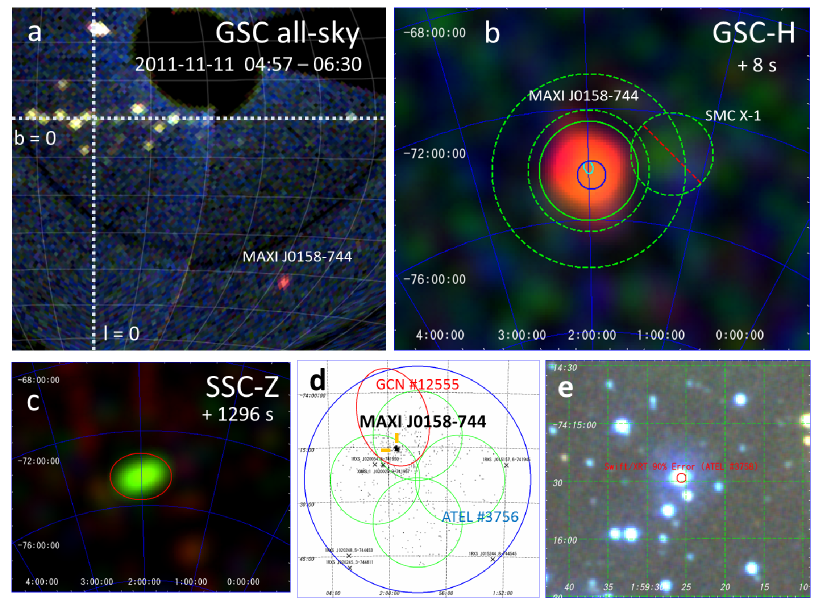
Figure 1: Images of MAXI J0158$-$744 taken by MAXI and Swift. (a) A part of the GSC all-sky image shown in Hammer-Aitoff projection of Galactic coordinates. Red, green, and blue color maps represent the intensities in 2$-$4, 4$-$10, and 10$-$20 keV bands, respectively. Grid lines are drawn every 1 h and 10^∘ in longitude and latitude, respectively. (b) Scan image of GSC-H around $T_{\rm trig}$. The source and background regions for the spectral analysis are shown in a green solid circle and dashed annulus, respectively. The excluded region centered at SMC X-1 is shown by a dashed circle. The colors represent the same energy bands as in a. The error regions reported in Kimura et al. (2011) and Morii et al. (2011a) are shown by a blue circle and cyan ellipse, respectively. Here, these error regions are made by adding the 90% confidence statistical error and the systematic uncertainty (0.1 deg, 90% containment radius). (c) Scan image of SSC-Z around $T_{\rm trig}+1296$ s. The source regions are shown by the red ellipses. Red, green, and blue color maps represent the intensities in 0.7$-$1, 1$-$4, and 4$-$10 keV bands, respectively. (d) Swift XRT mosaic image around MAXI J0158$-$744 obtained by the tiling observation data taken to search the X-ray counterpart (Kennea et al., 2011b). Green circles show FoVs of four Swift XRT pointings. The X-ray sources cataloged in ROSAT All-sky Survey and XMM-Newton Slew Survey are marked with X symbols. The same error regions as b are shown by blue circle and red ellipse. (e) Swift UVOT image made by combining the data with $v$, $b$, and $u$ filters, colored in red, green, and blue, respectively. The 90% confidence error circle obtained by Swift XRT is shown by a red circle.

2 Observation

MAXI J0158$-$744 (Kimura et al., 2011) was first detected during a MAXI GSC scan (Fig. 1b), centered at $T_{\rm trig}+8$ s within the $55$ s triangular transit response (See Fig. 9 in Sugizaki et al., 2011). It was subsequently detected twice by the MAXI SSC in scans at $+220$ s and $+1296$ s (Fig. 1c). Hereafter, we designate the MAXI scans by the mid-time of the scan transit, referred to $T_{\rm trig}$. Subsequent GSC scans to date (up to 2013 July 8) have failed to detect the source. In addition, the source had not been detected in prior GSC scans, since MAXI observations started on 2009 August 14 up to the previous scan at $-5530$ s. The MAXI observations around $T_{\rm trig}$ are summarized in Table 1.

Table 1: Summary of MAXI observation

Scan-ID	Scan Time(Start – End)(UT)	$\Delta t$(s)a	$t$(s)b	Detector	Fluxc
M$-1$d	2011-11-11 03:33:22 – 03:34:17∗	55	$-5530$	GSC-H	$<2.75\times 10^{-9}$$\,\,\,\,{}^{e,f}$
M+0	2011-11-11 05:05:39† – 05:06:34	55	$+8$	GSC-H	$1.81^{+0.14}_{-0.33}\times 10^{-8}$$\,\,\,\,{}^{g}$
M+1	2011-11-11 05:09:13 – 05:10:04	51	$+220$	SSC-H	$4.16^{+0.47}_{-1.20}\times 10^{-8}$$\,\,\,\,{}^{g}$
M+2	2011-11-11 05:27:09 – 05:28:00‡	51	$+1296$	SSC-Z	$1.57^{+0.17}_{-0.18}\times 10^{-8}$$\,\,\,\,{}^{h}$
M+3	2011-11-11 06:37:56§ – 06:38:51	55	$+5545$	GSC-H	$<9.60\times 10^{-10}$$\,\,\,\,{}^{e,f}$

Swift XRT performed follow-up observations from 0.44 days after $T_{\rm trig}$ (See Table 1 of Li et al., 2012). Swift UVOT also observed the optical counterpart in image mode. Swift UVOT grism observations were performed on 2011 November 19 (+8.23 days after $T_{\rm trig}$) and 2012 September 30 (324 days).

A ground-based optical spectrum, with relatively high resolution, was obtained on 2012 May 19 (190 days after the $T_{\rm trig}$) with the RC spectrograph on the SMARTS /CTIO 1.5m telescope; this is a long slit spectrograph oriented east-west (Walter et al., 2004, 2012). We used a 1 arcsec slit width and a Loral 1K CCD for the detector.

3 Analysis and results

3.1 Data analysis of MAXI GSC

On 2011 November 11, the position of MAXI J0158$-$744 was visible by three cameras of GSC-H (GSC_2, GSC_7 and GSC_8; Mihara et al., 2011; Sugizaki et al., 2011). One of these cameras (GSC_2) was operated at the nominal high voltage ($=1650$V), while the other two (GSC_7 and GSC_8) were operated at the reduced voltage ($=1550$V). We analyzed the GSC event data version 1.0 or later, which included the data taken by cameras operated at the nominal and reduced voltages. In these versions, the position and energy responses of the anodes #1 and #2 were significantly improved from the previous versions (0.x). We therefore used events taken from all anodes.

To make light curves within the interval of the scan-ID M+0 (Table 1), we followed the method shown in Morii et al. (2011b). Here we selected events within 5 mm of the position coincident with this source along the anode wires, which corresponds to about 2^∘ on the sky. The obtained light-curve data in energy bands of $2-4$, $4-10$, $10-20$, and $2-20$ keV were fitted with a model consisting of a triangular transit response curve for a point source with a constant flux and a constant background. The light curves are consistent with the model at the 90% confidence level, meaning that there was no significant variation of the source flux during that scan.

For the spectral analysis, we removed the GSC_8 data due to its poor response in the soft energy band. We selected a concentric circle and annulus centered at the target as the source and background regions, respectively. The radius of the source circle was set to 1.8 deg. The inner and outer radii of the background annulus were set to 2.2 and 3.5 deg, respectively. In both these regions, we excluded a circular region with a radius of 1.5^∘ centered at a near-by bright X-ray source, SMC X-1 (Fig. 1b). The spectrum and response files were made by the method described in Nakahira et al. (2011). The energy spectra obtained by the GSC Scan-ID M+0 are shown in Fig. 2 (left). We rebinned the data with a minimum of 1 count per energy bin and applied Cash statistics (Cash, 1979) in the fit. We used XSPEC v12.7.1 for the spectral analysis.

Since the location of this source is near the SMC, the interstellar absorption by the total Galactic H I column density towards this source, $N_{H}$, and optical extinction $E(B-V)$ are expected to be small. Thus, we decided to fix them for the following X-ray and optical spectral analysis. Two plausible different $N_{H}$ values are obtained from the HEASARC web site : $1.36\times 10^{21}$ cm^-2 by using LAB map (Kalberla et al., 2005) and $4.03\times 10^{20}$ cm^-2 by using DL map (Dickey & Lockman, 1990). The corresponding optical extinctions $E(B-V)$ are derived to be 0.28 and 0.084 mag, respectively, by using the relation with the H I column density (Bohlin, Savage & Drake, 1978). On the other hand, the map of dust infrared emission (Schlegel, Finkbeiner & Davis, 1998) suggests $E(B-V)=0.050$, which is closer to that from the DL map. Therefore, we decided to use the latter $N_{H}$ value, $4.03\times 10^{20}$ cm^-2, for the interstellar absorption. In the following, unabsorbed flux is corrected only for the interstellar absorption.

We fit the GSC X-ray spectrum with absorbed blackbody, power-law, thermal bremsstrahlung and Mekal (Mewe, Gronenschild & van den Oord, 1985) models from $2.0-10.0$ keV with $N_{H}$ fixed to $4.03\times 10^{20}$ cm^-2; the results are shown in Table 2. The spectrum is statistically consistent with all the models. Adopting the $N_{H}$ value of LAB map increases the unabsorbed flux by 2% from that using DL map. However, the difference in the spectral parameters and unabsorbed flux are negligibly small, when they are compared with the statistical uncertainty.

Figure 2: Energy spectra of MAXI J0158$-$744 observed by MAXI. (Top left) Crosses are the GSC-H spectrum at the scan of $+8$ s. The histogram is the best-fit blackbody model (Table 2). (Top middle) Crosses are the SSC-H spectrum at the scan of $+220$ s. The histogram is the best-fit blackbody model (Table 2). (Top right) Crosses are the SSC-Z spectrum at the scan of $+1296$ s. The histogram is the best-fit blackbody + Mekal model with parameters shown in Section 3.2.2. The Mekal component is shown by a dotted histogram. All the spectra are plotted binned with a minimum of 5 counts per energy bin. Backgrounds are subtracted. (Bottom) The residuals of the data from the models. Error bars, $1\sigma$.

Table 2: Spectral fitting parameters with 1$\sigma$ errors for the MAXI scans.

Model a	$\Gamma$b	$kT$c	$R_{\rm BB}$d	${\it EM}$e	abundf	Flux g	Luminosity h	C-stati
		(keV)	($\times 10^{3}$ km)	($\times 10^{63}$ cm-3)		(erg s-1 cm-2)	(erg s-1)	(DOFj)
MAXI GSC-H (Scan-ID M+0, $+8$ s)
PL	$4.89^{+0.29}_{-0.28}$	…	…	…	…	$6.92^{+0.55}_{-0.52}\times 10^{-9}$	$2.98^{+0.24}_{-0.22}\times 10^{39}$	43.4 (60)
BB	…	$0.45^{+0.03}_{-0.03}$	$1.26^{+0.29}_{-0.23}$	…	…	$6.74^{+0.27}_{-1.01}\times 10^{-9}$	$2.90^{+0.12}_{-0.43}\times 10^{39}$	51.8 (60)
TB	…	$0.93^{+0.10}_{-0.09}$	…	$5.9^{+2.1}_{-1.5}$	…	$6.84^{+0.31}_{-0.98}\times 10^{-9}$	$2.95^{+0.13}_{-0.42}\times 10^{39}$	45.3 (60)
Mekal	…	$0.94^{+0.08}_{-0.11}$	…	$4.3^{+1.6}_{-0.9}$	0.1 (fix)	$6.80^{+0.38}_{-0.67}\times 10^{-9}$	$2.93^{+0.17}_{-0.29}\times 10^{39}$	44.6 (60)
Mekal	…	$0.97^{+0.11}_{-0.10}$	…	$2.4^{+3.0}_{-2.1}$	$0.50^{+5.74}_{-0.50}$	$6.74^{+0.10}_{-5.14}\times 10^{-9}$	$2.90^{+0.04}_{-2.21}\times 10^{39}$	44.2 (59)
MAXI SSC-H (Scan-ID M+1, $+220$ s)
PL	$2.85^{+0.34}_{-0.32}$	…	…	…	…	$4.96^{+0.84}_{-0.84}\times 10^{-8}$	$2.13^{+0.36}_{-0.36}\times 10^{40}$	20.5 (36)
BB	…	$0.37^{+0.05}_{-0.05}$	$4.8^{+1.6}_{-1.2}$	…	…	$4.16^{+0.47}_{-1.20}\times 10^{-8}$	$1.79^{+0.20}_{-0.52}\times 10^{40}$	30.2 (36)
TB	…	$1.46^{+0.50}_{-0.35}$	…	$4.5^{+1.7}_{-1.2}$	…	$4.71^{+0.56}_{-1.13}\times 10^{-8}$	$2.03^{+0.24}_{-0.49}\times 10^{40}$	22.5 (36)
Mekal	…	$1.61^{+0.48}_{-0.36}$	…	$3.4^{+0.7}_{-0.6}$	0.1 (fix)	$4.71^{+0.64}_{-0.87}\times 10^{-8}$	$2.03^{+0.28}_{-0.37}\times 10^{40}$	24.0 (36)
Mekal	…	$1.51^{+0.44}_{-0.41}$	…	$4.1^{+1.5}_{-1.0}$	$<0.25$(90%)	$4.77^{+1.36}_{-0.83}\times 10^{-8}$	$2.05^{+0.59}_{-0.36}\times 10^{40}$	22.6 (35)
MAXI SSC-Z (Scan-ID M+2, $+1296$ s)
PL	$3.19^{+0.26}_{-0.24}$	…	…	…	…	$1.71^{+0.20}_{-0.18}\times 10^{-8}$	$7.37^{+0.87}_{-0.78}\times 10^{39}$	83.4 (69)
BB	…	$0.33^{+0.03}_{-0.03}$	$2.29^{+0.48}_{-0.39}$	…	…	$1.50^{+0.10}_{-0.28}\times 10^{-8}$	$6.48^{+0.45}_{-1.21}\times 10^{39}$	84.2 (69)
TB	…	$0.94^{+0.17}_{-0.14}$	…	$2.61^{+0.71}_{-0.54}$	…	$1.61^{+0.12}_{-0.30}\times 10^{-8}$	$6.91^{+0.50}_{-1.30}\times 10^{39}$	80.8 (69)
Mekal	…	$1.03^{+0.10}_{-0.09}$	…	$1.42^{+0.18}_{-0.16}$	0.1 (fix)	$1.57^{+0.17}_{-0.18}\times 10^{-8}$	$6.75^{+0.73}_{-0.77}\times 10^{39}$	80.8 (69)
Mekal	…	$0.96^{+0.13}_{-0.10}$	…	$1.86^{+0.57}_{-0.46}$	$0.041^{+0.058}_{-0.031}$	$1.58^{+0.11}_{-0.45}\times 10^{-8}$	$6.80^{+0.49}_{-1.93}\times 10^{39}$	79.4 (68)

3.2 Data analysis of MAXI SSC

After the first detection of MAXI J0158$-$744 with the MAXI GSC scan at $+8$ s, MAXI SSC detected this source twice as shown in Table 1. Before $+8$ s, MAXI J0158$-$744 was below the SSC detection limit of $\sim$200 mCrab in each night scan. For the spectral analysis, we selected the source regions as shown in Fig. 1c and reduced the SSC events in the same way as Kimura et al. (2012). While the second SSC detection at $+1296$ s was done at night in the orbit, the first SSC at $+220$ s was done at the day-time. Since the SSC day-time data were contaminated by the visible/infrared light from the Sun (Tsunemi et al., 2010), we have to be careful of the analysis of the $+220$ s scan data. We estimated the area suffering from the contamination based on the event distribution, which led to the decision that 63% of the source area was not suitable for the spectral analysis. We thus used data from the remaining 37% area in the analysis.

The energy spectra obtained by the SSC scans at $+220$ s and $+1296$ s are shown in Fig. 2 (middle, right). In the latter spectrum, since emission lines seemed to be present, we analyzed the SSC spectra with special care by following the method shown in “low count spectra” of the XSPEC wiki site . To avoid losing information on emission lines due to the spectral binning, we did not bin the data and applied Cash statistics (Cash, 1979) to the fits. We fit the source spectra with a model consisting of a source and a background component. Here, the background model was analytically-described to approximate the actual background spectrum in $0.7-7.0$ keV. It was constructed by averaging the two year SSC data weighted with geomagnetic cut-off-rigidity, because the background events are caused by charged particles and cosmic diffuse X-rays. The details of the background spectrum are shown in Kimura et al. (2012). We fit the spectra by absorbed blackbody, power-law, thermal bremsstrahlung and Mekal (Mewe, Gronenschild & van den Oord, 1985) models in $0.7-7.0$ keV with $N_{H}$ fixed to $4.03\times 10^{20}$ cm^-2 (Section 3.1) and the results are shown in Table 2. For the Mekal model we let the abundance parameter (hereafter, we abbreviate it to abund.) be free or fixed to 0.1 (a typical abundance of the SMC; Carrera et al., 2008). For the first SSC spectrum ($+220$ s), the data are statistically consistent with all the models, while for the second, the free abundance Mekal model is preferred. Adopting the $N_{H}$ value of LAB map increases the unabsorbed fluxes by up to 20% from those using DL map. However, differences in all the spectral parameters and unabsorbed fluxes are not significant (less than 2.6 sigma level of the statistical uncertainty).

As shown in Table 2, the initial X-ray outburst of MAXI J0158$-$744 detected by MAXI GSC and SSC was peaked at $+220$ s. The peak luminosity was extraordinarily luminous, $2\times 10^{40}$ erg s^-1 in $0.7-7.0$ keV, which is two orders of magnitude larger than the Eddington luminosity of a solar mass object. In the following subsections, we investigate the MAXI SSC spectrum at $+1296$ s, where emission lines are apparent, with two scenarios: shock-induced emission and photospheric emission at the fireball phase (See Section 4).

3.2.1 Detailed spectral analysis of MAXI SSC at $+1296$ s with a shock-induced emission model

To investigate the emission lines in the spectrum at $+1296$ s, we first fit the spectrum with models consisting of thermal bremsstrahlung continuum and Gaussian lines, whose widths were fixed to be small against the detector energy resolution, 85 eV (FWHM) at 1.0 keV (Kimura et al., 2012). The best-fit parameters are summarized in Table 3 (upper) and the models are shown in Fig. 3 (abcd). The results of the likelihood ratio tests (Cash, 1979) in the last two rows of Table 3 (upper) indicate that the addition of the Gaussian lines at the energies $E_{1}$, $E_{2}$ and $E_{3}$ one by one improves the fits with a chance probability of 0.0044, 0.084 and 0.085, respectively. The line at the energy $E_{1}$ is the most significant, and is inferred to be a resonance line of He-like neon (0.922 keV). The other two lines are less significant than $2\sigma$ and no corresponding major lines exist at these energies. However, the line center energy $E_{2}$ may suggest a radiative recombination continuum of He-like neon (1.20 keV) or Lyman beta line of H-like neon (1.24 keV), and the $E_{3}$ may suggest a resonance line of He-like aluminum (1.60 keV) or $1s3p$ ${}^{1}P_{1}$ $\rightarrow$ $1s^{2}$ ${}^{1}S_{0}$ line of He-like magnesium (1.58 keV). The neon emission line suggests that the initial bright outburst would have been produced by an optically-thin thermal emission mechanism, whose site was a region heated by the shock wave of a nova explosion as seen in some novae (RS Ophiuchi and V407 Cyg; Sokoloski et al., 2006; Nelson et al., 2012).

Table 3: Spectral fitting parameters of a continuum + emission lines for the SSC-Z scan at $+1296$ s and the likelihood ratio test.

Model	TBa	TB + Lineb	TB + 2 Lines	TB + 3 Lines
$kT$c (keV)	$0.94^{+0.17}_{-0.14}$	$1.12^{+0.25}_{-0.19}$	$1.21^{+0.34}_{-0.20}$	$1.28^{+0.36}_{-0.25}$
${\it EM}$d ($\times 10^{63}$ cm-3)	$2.61^{+0.71}_{-0.54}$	$1.78^{+0.53}_{-0.40}$	$1.42^{+0.44}_{-0.37}$	$1.17^{+0.43}_{-0.32}$
$E_{1}$e (keV)	…	$0.93^{+0.01}_{-0.01}$	$0.93^{+0.01}_{-0.01}$	$0.93^{+0.01}_{-0.01}$
$EW_{1}$f (keV)	…	$0.19^{+0.13}_{-0.07}$	$0.26^{+0.22}_{-0.10}$	$0.33^{+0.26}_{-0.11}$
$E_{2}$g (keV)	…	…	$1.19^{+0.02}_{-0.02}$	$1.19^{+0.02}_{-0.02}$
$EW_{2}$ (keV)	…	…	$0.14^{+0.14}_{-0.08}$	$0.18^{+0.20}_{-0.08}$
$E_{3}$h (keV)	…	…	…	$1.57^{+0.03}_{-0.04}$
$EW_{3}$ (keV)	…	…	…	$0.24^{+0.26}_{-0.14}$
$C$-stati(DOFj)	342.9(1723)	332.1(1721)	327.1(1719)	322.2(1717)
$\Delta C$($\Delta$DOF)k	…	10.8(2)	5.0(2)	4.9(2)
$P$-valuel	…	0.0044	0.084	0.085
Model	BBm	BB + Line	BB + 2 Lines	BB + 3 Lines
$kT$c (keV)	$0.33^{+0.03}_{-0.03}$	$0.38^{+0.04}_{-0.03}$	$0.41^{+0.04}_{-0.04}$	$0.42^{+0.05}_{-0.04}$
$R_{\rm BB}$n ($\times 10^{3}$ km)	$2.29^{+0.48}_{-0.39}$	$1.54^{+0.35}_{-0.28}$	$1.22^{+0.35}_{-0.23}$	$1.10^{+0.35}_{-0.22}$
$E_{1}$e (keV)	…	$0.93^{+0.01}_{-0.01}$	$0.93^{+0.01}_{-0.01}$	$0.93^{+0.01}_{-0.01}$
$EW_{1}$f (keV)	…	$0.32^{+0.21}_{-0.11}$	$0.45^{+0.36}_{-0.14}$	$0.55^{+0.45}_{-0.18}$
$E_{2}$g (keV)	…	…	$1.19^{+0.02}_{-0.02}$	$1.19^{+0.02}_{-0.02}$
$EW_{2}$ (keV)	…	…	$0.16^{+0.16}_{-0.08}$	$0.20^{+0.21}_{-0.09}$
$E_{3}$h (keV)	…	…	…	$1.57^{+0.04}_{-0.05}$
$EW_{3}$ (keV)	…	…	…	$0.16^{+0.22}_{-0.11}$
$C$-stati(DOFj)	343.8(1723)	326.7(1721)	321.1(1719)	318.2(1717)
$\Delta C$($\Delta$DOF)k	…	17.1(2)	5.6(2)	2.9(2)
$P$-valuel	…	$1.9\times 10^{-4}$	0.061	0.23

Figure 3: MAXI SSC-Z spectrum of MAXI J0158$-$744 at $+1296$ s. (a, c) The histograms are the best-fit thermal bremsstrahlung (a) and thermal bremsstrahlung + 3 Gaussian lines models (c). (e) The histogram is the best-fit Mekal_LT + Mekal_HT model, where the abunds of Ne and the other elements in the Mekal_LT component are set to 0.1 and 0.1, respectively (Table 4, the first row). (g) The histogram is the same model as e, where these abunds are set to 10.0 and 0.1 (Table 4, the fifth row). All the spectra are plotted binned with a minimum of 5 counts per energy bin. (b, d, f, h) The residuals of the data from the models. Error bars, 1 $\sigma$.

We next tried to fit the spectrum with more physically motivated models. Although it can be fit with an optically-thin thermal emission model (Mekal in XSPEC terminology) with a temperature of $\sim 1.0$ keV (Table 2), the model cannot produce the observed strong He-like neon line. To reproduce the He-like neon, another optically-thin thermal component with a lower temperature (about 0.1 keV) is necessary. Thus, we examined a model consisting of two Mekal models (Mekal_LT + Mekal_HT), whose temperatures are $\sim 0.1$ keV in the lower component (LT) and $\sim 1.0$ keV in the higher component (HT), respectively. The best-fit result in Table 2 shows that the abund of the Mekal_HT is consistent with that of the SMC. This conclusion, however, is not completely correct, because the fit included an energy range affected by the He-like neon line produced by the Mekal_LT component. To determine the abund of Mekal_HT, we fit the spectrum excluding the energy range $0.8-1.0$ keV, and then obtained an upper limit for the abund of 0.25 (90% confidence limit), which is consistent with that of the SMC (Carrera et al., 2008). We thus decided to fix the abund of the Mekal_HT component to 0.1. For the Mekal_LT component, the observed strong He-like neon line suggests a large abundance for neon. We postulate that the Mekal_LT component was produced in a reverse shocked region whose material was ejecta from the nova explosion (See Section 4).

To estimate the abunds of the Mekal_LT component, we fit the spectrum with the Mekal_LT + Mekal_HT model assuming six combinations of the abunds of neon and the other elements for Mekal_LT as shown in Table 4. Here, at the first step in the spectral fit, we let the temperature and emission measure of the Mekal_HT component freely vary. When the 1$\sigma$ error range of the temperature of the Mekal_LT was not constrained to less than 0.3 keV in the first step (the first three cases of Table 4), we fixed the temperature of Mekal_HT and then the emission measure of Mekal_HT to the best-fit values. These best fit values were obtained by fitting the same spectrum, excluding the energy range $0.8-1.0$ keV, with a single Mekal component and the abund fixed to 0.1. For the first case of Table 4, the 1$\sigma$ error range of the Mekal_LT could not be constrained to be less than 0.3 keV, even after both the temperature and emission measure of Mekal_HT were fixed. Figure 3 (efgh) presents the difference in these spectral fits with respect to the neon abunds of the Mekal_LT component. As a result, the neon abund of the Mekal_LT was suggested to be much higher than that of the SMC (Table 4), and it indicates that the Mekal_LT component originates in ejecta from the nova. The unabsorbed flux in $0.7-7.0$ keV, assuming the Mekal_LT + Mekal_HT model with parameters shown in the fifth row of Table 4 (the best-fit model), is $1.63^{+0.19}_{-0.17}\times 10^{-8}$ erg s^-1 cm^-2.

Table 4: Spectral fitting parameters of the Mekal_LT^a + Mekal_HT^b model for the SSC-Z scan at $+1296$ s with 1$\sigma$ errors.

abundc		$kT$(LTd)	${\it EM}$(LT)	$kT$(HTe)	${\it EM}$(HT)	C-statf
Ne	Others	(keV)	($\times 10^{63}$ cm-3)	(keV)	($\times 10^{63}$ cm-3)	(DOFg)
$0.1$	$0.1$	0.13h(unconstrained)i	11.5h(0.0 $-$ 194)j	$1.29$ (fix)k	$1.19$ (fix)k	81.6 (69)
$1.0$	$1.0$	$0.14^{+0.11}_{-0.05}$	$1.83^{+18.87}_{-1.80}$	$1.29$ (fix)k	$1.19$ (fix)k	80.6 (69)
$10.0$	$10.0$	$0.13^{+0.08}_{-0.05}$	$0.19^{+1.88}_{-0.18}$	$1.29$ (fix)k	$1.19$ (fix)k	80.5 (69)
$1.0$	$0.1$	$0.13^{+0.06}_{-0.04}$	$10.3^{+184.5}_{-8.3}$	$1.44^{+0.16}_{-0.28}$	$1.03^{+0.24}_{-0.12}$	74.8 (67)
∗$10.0$	$0.1$	0.13h($0.0808^{l}-0.24$)j	$1.43^{+58.32}_{-1.30}$	$1.44^{+0.17}_{-0.21}$	$1.02^{+0.20}_{-0.09}$	73.8 (67)
$10.0$	$1.0$	$0.13^{+0.06}_{-0.04}$	$1.11^{+21.24}_{-0.87}$	$1.42^{+0.17}_{-0.25}$	$1.05^{+0.20}_{-0.15}$	74.6 (67)

3.2.2 Detailed spectral analysis of MAXI SSC at $+1296$ s with photospheric emission at the fireball phase

The initial bright outburst detected by MAXI may also be explained by photospheric emission at the ignition phase of a nova explosion, the so-called fireball phase (See Section 4). In this scenario, the main continuum component in the spectrum of MAXI SSC at $+1296$ s is blackbody emission, while the emission lines come from the optically-thin region surrounding the photosphere (See Fig. 5 in Section 4). Thus, we fit the spectrum with models consisting of blackbody continuum and Gaussian lines. The results of the fit are shown in Table 3 (lower). The addition of the Gaussian line at the energy $E_{1}$ significantly improves the fits with a chance probability of $1.9\times 10^{-4}$, while the other two lines are detected at $<2\sigma$. The identifications of these lines are the same as in Section 3.2.1. The detection of the neon emission line suggests that the spectrum contains an optically-thin thermal emission component. Therefore, this spectrum could be explained by a composite model of a blackbody and a Mekal with a temperature below 0.3 keV, and an exceptionally large neon abundance, similar to the two Mekal models in Section 3.2.1. When the abunds of neon and the other elements are set to $10$ and 0.1, respectively, the resultant best-fit spectral parameters are as follows: the temperature and emission measure of the Mekal component are 0.14($0.0808-0.28$) keV (See footnotes $h$, $j$ and $l$ of Table 4) and $1.13^{+62.97}_{-1.03}\times 10^{63}$ cm^-3, respectively. The temperature and radius of the blackbody component are $0.39^{+0.04}_{-0.04}$ keV and $1.47^{+0.37}_{-0.31}\times 10^{3}$ km, respectively.

3.3 Upper limits on other MAXI GSC scans

In the scans at $-5530$ s and $+5545$ s (Table 1), MAXI J0158$-$744 was not detected by MAXI GSC. To calculate the upper limits on these fluxes, we assumed the best-fit Mekal_LT + Mekal_HT model obtained by the MAXI SSC scan at $+1296$ s (Section 3.2.1) and the best-fit blackbody model (the Scan-ID M+1 in Table 2). In the former model, the abund of the Mekal_HT and the Mekal_LT was fixed to 0.1 except for the neon abund in the Mekal_LT fixed to 10 (Table 4, the fifth row). The 90% confidence-level upper limits on the unabsorbed flux in $0.7-7.0$ keV for these scans are $<1.94\times 10^{-9}$ and $<8.29\times 10^{-10}$ erg s^-1 cm^-2 in the two Mekal model, and $<2.75\times 10^{-9}$ and $<9.60\times 10^{-10}$ erg s^-1 cm^-2 in the blackbody model.

In addition, in all five scans between the scan at $+5545$ s (+0.064 d) and the start of the Swift XRT follow-up (i.e. at +0.128, +0.192, +0.256, +0.320, and +0.385 days), MAXI J0158$-$744 was not detected by MAXI GSC. The 90% confidence-level upper limit on the unabsorbed flux in the 0.7$-$7.0 keV band for this period was $3.5\times 10^{-10}$ erg s^-1 cm^-2, assuming the former model and $2.5\times 10^{-10}$ erg s^-1 cm^-2 for the latter model.

3.4 Analysis of follow-up observations

3.4.1 Analysis of Swift observations

We analyzed the same Swift XRT archival data as listed in Table 1 of Li et al. (2012), using Swift software version 3.9, released as part of HEASOFT 6.12. We extracted the source events from a circle with optimal radii ($47^{\prime\prime}-23^{\prime\prime}$) and the background from an offset circular region of radius 142^′′. For the data on day 0.54, we excluded events from the inner 5^′′ of the PSF to avoid pile-up. In the spectral fit, we used the RMFs (Redistribution Matrix Files) of swxpc0to12s6_20010101v013.rmf in PC mode and swxwt0to2s6_20010101v014.rmf in WT mode. The ARFs (Ancillary Response Files) were generated by using the commands xrtexpomap (to create the exposure maps) and xrtmkarf.

We fit the Swift XRT spectra with absorbed blackbody or Mekal models with the intrinsic column $N_{H}$ allowed to vary. These models include two absorption components: the interstellar absorption $N_{H}$ fixed at $4.03\times 10^{20}$ cm^-2 (Section 3.1) and intrinsic absorption. In the Mekal model, the abund was fixed to 0.1, a typical abund of the SMC (Carrera et al., 2008, See also Section 3.2.1). The unabsorbed flux obtained by the blackbody fits are shown in Figure 4.

We also analyzed the Swift UVOT data obtained at the same time as Swift XRT, using the Swift software version 3.9, released as part of HEASOFT 6.12. The image data of each filter, from each observation sequence, i.e., with a given observation ID, were summed using uvotimsum. However, for images taken within 2 days of the outburst ($b$, $u$ and $w1$ bands) individual exposures were long enough that summing was not necessary. Photometry of the source in individual sequences was derived via uvotmaghist, using an extraction region of radius 5^′′ and a suitable background region. Magnitudes are based on the UVOT photometric system (Poole et al., 2008). XSPEC compatible spectral files for the source were created using the same region with uvot2pha.

The $u$ band light curve is shown in Figure 4. We calculated the absolute magnitude of the enhanced emission after extinction correction, where $E(B-V)=0.050$ mag (Section 3.1), $A_{V}/E(B-V)=3.1$, $A_{u}=1.664A_{V}$ (Schlegel, Finkbeiner & Davis, 1998), and the SMC distance of $d=60$ kpc were assumed. Here, we subtracted the flux in the plateau phase ($13.58$ mag, average of $u$-band magnitudes from 11.65 days to 27.86 days.). By fitting it with a linear function, we obtained the absolute magnitude of $-5.04\pm 0.07$ mag at 0.44 day and the speed class indicator parameter defined by the time to decline 2 mag from maximum (Warner, 2008), $t_{d,2}=1.9\pm 0.2$ ($1\sigma$) days. This classifies the event as a “very fast nova” (Warner, 2008), assuming that the optical enhancement was due to the photospheric emission as in usual novae.

To investigate the optical enhanced emission, we made a difference spectrum from the Swift UVOT photometry over the six filter bandpasses between day 1.5 and 149, and we fit it with a blackbody model with fixed interstellar extinction (Section 3.1). The blackbody temperature of $1.22^{+0.11}_{-0.10}\times 10^{4}$ K and the radius of $6.58^{+1.03}_{-0.89}\times 10^{11}$ cm were obtained at the best fit. We also fit the spectrum from day 149 with the blackbody model, obtaining a temperature of $2.34^{+0.04}_{-0.04}\times 10^{4}$ K and a radius of $5.81^{+0.14}_{-0.14}\times 10^{11}$ cm. The extrapolation of the best-fit blackbody spectrum towards the UV region is consistent with the UV flux obtained by Galaxy Evolution Explorer (GALEX; Morrissey et al., 2005) during the pre-outburst phase (Li et al., 2012). In addition, Li et al. (2012) reported that the I-band flux returned to the pre-outburst level $\sim 60$ days after $T_{\rm trig}$. So, we can assume that the flux at day 149 contains only emission from the binary companion star. The obtained temperature and radius are consistent with those of a B-type star, as shown in Li et al. (2012).

Swift UVOT grism spectra are close to that of an early B-type star. No clear emission lines can be identified above the noise, as shown in Li et al. (2012).

3.4.2 Ground-based optical spectroscopy by SMARTS

We obtained three 200-s spectra of the optical counterpart of MAXI J0158$-$744 in order to filter for cosmic rays. We combine the three images, and extract the spectrum by fitting a Gaussian in the spatial direction at each pixel. Wavelength calibration is accomplished by fitting a 3^rd to 6^th order polynomial to the calibration lamp line positions. The optical spectrum covers nearly the entire optical band ($3300-9500\AA$) at $17\AA$ resolution.

There are clear emission lines of $H_{\alpha}$ and $H_{\beta}$, with equivalent widths of $16$ $\AA$ and $1$ $\AA$, respectively. We could not find any other significant emission or absorption lines above the noise level. The SMARTS spectrum matches the NTT spectrum of Li et al. (2012), albeit with worse signal to noise.

3.5 Historical X-ray fluxes

To investigate the activity of MAXI J0158$-$744 before the discovery, we searched for previous X-ray observations of the area including the target position. This region was observed by the ROSAT all-sky survey, XMM-Newton slew survey and MAXI GSC. The source was undetected in all these observations. We calculated the upper limits on the unabsorbed fluxes in an energy range of $0.7-7.0$ keV, assuming the best-fit Mekal_LT + Mekal_HT model (Table 4, the fifth row; Outburst Model) and a typical spectrum in the SSS phase observed by Swift XRT, an absorbed blackbody with a temperature of 0.1 keV (SSS Model; Li et al., 2012).

The ROSAT All-Sky Survey covered this field, with an exposure of 775 s in total between 1990 September 22 and December 3. These data provide a PSPC count rate upper limit of $0.14$ counts s^-1 (90% confidence limit) over $0.1-2.5$ keV; corresponding to $<2.1\times 10^{-13}$ and $<6.5\times 10^{-14}$ ergs cm^-2 s^-1 ($0.7-7.0$ keV), assuming Outburst Model and SSS Model, respectively (Table 5).

XMM-Newton slewed over the source three times on 2006 November, 2007 October, and 2009 November. We obtained EPIC pn count rate upper limits of 0.35, 1.5 and 0.50 counts s^-1 ($2\sigma$ level) in $0.2-12$ keV, respectively. The corresponding unabsorbed fluxes ($0.7-7.0$ keV) are shown in Table 5.

We also analyzed the MAXI GSC image in the 4$-$10 keV band integrated for 7 months from 2009 September 1 to 2010 March 31. Applying the same analysis procedure as used by Hiroi et al. (2011), we obtain a 90% confidence-level upper limit of 0.10 mCrab. It corresponds to an unabsorbed flux of $<1.8\times 10^{-11}$ ergs cm^-2 s^-1 ($0.7-7.0$ keV), assuming Outburst Model.

Table 5: Summary of ROSAT all-sky survey and XMM-Newton slew survey observations.

Date	Telescope	Exp.(s)a	Flux(Outburst)b	Flux(SSS)b
1990-09-22 – 1990-12-03	ROSAT	775	$<2.1\times 10^{-13}$	$<6.5\times 10^{-14}$
2006-11-01 10:03:35	XMM-Newton	8.9	$<3.6\times 10^{-13}$	$<7.3\times 10^{-14}$
2007-10-28 11:57:17	XMM-Newton	2.1	$<1.6\times 10^{-12}$	$<3.2\times 10^{-13}$
2009-11-30 23:41:46	XMM-Newton	6.1	$<5.2\times 10^{-13}$	$<1.1\times 10^{-13}$

Figure 4: Evolution of the fluxes of MAXI J0158$-$744. (Top, Middle) The X-ray luminosity with horizontal axes in linear (top) and log (middle) scales. Here, the source distance is assumed to be the SMC distance of 60 kpc. (Bottom) The $u$ band magnitude. The squares, circles and triangles show the data obtained by MAXI GSC (Sections 3.1 and 3.3), MAXI SSC (Sections 3.2 and 3.2.2) and Swift (Section 3.4), respectively. For the MAXI data, the luminosities converted from the fluxes of Table 1 and Section 3.3 are shown. For the Swift XRT data, those obtained by blackbody fits are shown (Section 3.4). The vertical error bars represent $1\sigma$ level. Horizontal dashed and dotted lines show the 90% confidence upper limits obtained by XMM-Newton slew survey and ROSAT PSPC, respectively, assuming SSS Model (Section 3.5).

4 Discussion

The X-ray transient MAXI J0158$-$744 is characterized by (1) a soft X-ray spectrum with most of the X-ray photons being detected below 4 keV (Fig. 1 and Fig. 2), (2) a short duration (between $t_{2}-t_{1}=1.3\times 10^{3}$ s and $t_{3}-t_{-1}=1.10\times 10^{4}$ s; Table 1), (3) a very rapid rise time ($<t_{1}-t_{\rm-1}=5.5\times 10^{3}$ s; Table 1), and (4) a huge peak luminosity of $2\times 10^{40}$ erg s^-1 in the $0.7-7.0$ keV band recorded at the second MAXI scan. The unusually soft spectrum of the outburst is beyond astronomers’ expectations, because most short-lived luminous transient X-ray sources are hard X-ray emitters, e.g. Gamma-ray Bursts (Band et al., 1993), Soft Gamma Repeaters (Woods & Thompson, 2006), Super-giant Fast X-ray Transients (Sguera et al., 2006), and X-ray bursts (Galloway et al., 2008). The discovery of MAXI J0158$-$744, together with supernova shock breakouts (Soderberg et al., 2008), suggests that the wide-field monitoring experiments in soft X-rays ($<2$ keV) will open new discovery fields.

Li et al. (2012) reported the optical spectra obtained by SAAO and ESO, showing that the source is a Be star. In addition, they showed that the radial velocity of this source is consistent with the SMC, which strongly supports that this source is located in the SMC. Due to the similarity between the Swift X-ray spectra and the SSS phase of novae, they concluded that this source is a binary system consisting of a WD and a Be star. We also analyzed the SED of the optical counterpart and found that it is consistent with that of a B-type star. The optical spectrum taken by SMARTS showed clear emission lines of $H_{\alpha}$ and $H_{\beta}$, confirming the conclusion of Li et al. (2012).

We fit the Swift XRT spectra with absorbed blackbody or Mekal models. Neither model was strongly preferred from the statistics. However, the evolution of the temperature of the Mekal model shows an unexplained decrease at 3$-$7 days, while the temperature and radius of the blackbody fits can be understood as being due to the shrinking photosphere. Here, the radius decreased from $\sim 10^{4}$ km to $\sim 100$ km, while the temperature increased from $\sim 0.06$ keV to $\sim 0.1$ keV. Therefore, we conclude that the spectra were basically blackbody-like, and hence can be identified as a super-soft X-ray phase of a nova. This conclusion is the same as Li et al. (2012). Fits using WD atmosphere models (Rauch et al., 2010; van Rossum, 2012) would allow further insights, although a trial with the Tübingen WD model failed to improve the fits, due to the computational upper limit for the temperature (Li et al., 2012). Probably, more sophisticated spectral models like atmosphere models would improve the fits. Li et al. (2012) reported that adding a broad emission line at $\sim$0.7 keV and an absorption edge at $0.89$ keV improves the fit for the spectrum at $1.54$ d significantly, which also supports our interpretation that the early X-ray emission is due to the SSS phase of novae.

The SSS phase spectra from the first Swift XRT follow-up observation at $0.44$ d and the simultaneous optical enhanced emission obtained by Swift UVOT are unusual in the evolution of standard novae. Nonetheless, if the optical enhanced emission is the photospheric emission of nova ejecta as in standard novae, the speed class indicator parameter of $t_{d,2}$ means that it is the second fastest nova next to U Sco ($1.2$ days; Schwarz et al., 2011) and an equal record to V838 Her ($2$ days; Schwarz et al., 2011). The peak absolute magnitude ($-5.04\pm 0.07$) at 0.44 day in the first Swift UVOT observation is four magnitudes fainter than those of typical novae ($-9.016\pm 0.008$), expected from the MMRD (maximum magnitude - rate of decline) relation (della Valle & Livio, 1995). If this enhanced optical emission was photospheric emission from the nova ejecta, it suggests a low ejecta mass in this nova explosion. In the subsequent discussion below, we will show that the enhanced optical emission is not photospheric emission, however, the conclusion of the low ejecta mass remains correct.

4.1 Shock heating mechanism

Optically-thin thermal X-ray emission of novae is usually explained by a shock heating mechanism at a blast wave produced by the nova explosion. The recurrent nova, RS Ophiuchi, in 2006 exhibited the most luminous optically-thin thermal X-ray emission ($1\times 10^{36}$ erg s^-1) among novae that has ever been observed (Sokoloski et al., 2006). The luminosity of the X-ray outburst of MAXI J0158$-$744 was, surprisingly, four orders of magnitude larger than this. Li et al. (2012) explained the luminosity of MAXI J0158$-$744 by the shock heating mechanism, however, their explanation has difficulties as follows. They tried to explain the observed luminosity of $\sim 10^{39}$ erg s^-1 at the time of the first GSC scan (scan-ID M+0; Table 1) using Equation (1) of Li et al. (2012), where the radius of the shock wave $r_{s}\sim 1.5\times 10^{13}$ cm is assumed. However, in order for the shock wave to expand to this radius within $\Delta t_{r}=t_{1}-t_{\rm-1}=5.5\times 10^{3}$ s (Table 1), the shock wave velocity must be exceptionally large ($V_{s}=r_{s}/\Delta t_{r}\sim 3\times 10^{4}$ km s^-1) for novae. In addition, if the velocity of the shock wave was such a large value, the temperature of the plasma thermalized by the shock wave becomes very high ( $kT=\frac{3m_{p}\mu{V_{s}}^{2}}{16}\sim 1$ MeV, where $m_{p}$ is the proton mass, and $\mu$ is the mean molecular weight ), which is contradictory to the observed soft spectrum of the outburst ($kT\sim 1$ keV).

We further discuss the shock heating scenario, considering the very rapid rise time within $\Delta t_{r}$ s and the observed low temperature ($0.97$ keV; Table 2). We set the onset time of the nova explosion $t_{0}$ between the last scan time of the scan-ID M$-1$ ($t_{\rm-1}$; Table 1) and the first scan time of the scan-ID M+0 ($t_{1}$; Table 1). The elapsed time from $t_{0}$ to $t_{1}$ is $t_{{\rm e},1}=t_{1}-t_{0}<\Delta t_{r}$ s. We check whether the observed emission measure (${\it EM}\equiv\int n_{e}n_{p}dV=1.0\times 10^{63}\,{\it EM}_{63}\,{d_{60}}^{2}$ cm^-3, where ${\it EM}_{63}=2.4$ for the Mekal model fit with free abund in Table 2 and $d_{60}\simeq 1$; here $n_{e}$ and $n_{p}$ are the number densities of electrons and protons, respectively) can be produced at $t_{{\rm e},1}$ by considering two simple geometries, a filled sphere and spherical shell. Here, we assume the circumbinary space is filled with a fully-ionized electron-ion plasma with a constant density. We assume the constant shock velocity $V_{s}$, and then the distance ($R_{1}$) of the shock wave front reaching from the surface of the WD at the time $t_{{\rm e},1}$ is

$$R_{1}=t_{{\rm e},1}\times V_{s}<\Delta t_{r}\times V_{s}=5.5\times 10^{11}V_{s3}\,\,\,{\rm cm},$$ (1)

where $V_{s}=10^{3}V_{s3}$ km s^-1 ($V_{s3}\simeq 1$).

If the shape of the emission region is a filled sphere, the emission measure at $t_{{\rm e},1}$ is written as ${\it EM}=\frac{4}{3}\pi{R_{1}}^{3}{n_{p}}^{\prime}{n_{e}}^{\prime}=\frac{4}{3}\pi{R_{1}}^{3}f_{a1}{{n_{p}}^{\prime}}^{2}$ (hereafter, we add “  ^′  ” for the physical value after the shock). Since we assume that the initial X-ray outburst is an optically-thin emission, the condition of the optical depth is ${n_{e}}^{\prime}\sigma_{T}R_{1}=f_{a1}{n_{p}}^{\prime}\sigma_{T}R_{1}<1$, where $\sigma_{T}$ is the Thomson cross section. By removing ${n_{p}}^{\prime}$, we obtain $R_{1}>\frac{3{\it EM}}{4\pi}\sigma_{T}^{2}f_{a1}=1.1\times 10^{14}f_{a1}{\it EM}_{63}{d_{60}}^{2}~{}{\rm cm}$. Therefore, it is impossible to produce the observed emission measure at $t_{1}$ in the usual shock velocity ($V_{s3}\sim 1-10$; Schwarz et al., 2011; Warner, 2008), even at the speed of light.

Next, if the shape of the emission region is a spherical shell with a depth of $\delta R_{1}$, the emission measure at $t_{{\rm e},1}$ is written as ${\it EM}=4\pi{R_{1}}^{2}\delta R_{1}{n_{p}}^{\prime}{n_{e}}^{\prime}$. The condition of the optical depth is ${n_{e}}^{\prime}\sigma_{T}\delta R_{1}=f_{a1}{n_{p}}^{\prime}\sigma_{T}\delta R_{1}<1$. By removing ${n_{p}}^{\prime}$, we obtain $R_{1}>\frac{{\it EM}}{4\pi}\sigma_{T}^{2}\frac{\delta R_{1}}{R_{1}}f_{a1}=3.6\times 10^{13}f_{a1}{\it EM}_{63}{d_{60}}^{2}\frac{\delta R_{1}}{R_{1}}~{}{\rm cm}$. Using Condition 1, the depth of the shell is limited to $\frac{\delta R_{1}}{R_{1}}<1.5\times 10^{-2}{d_{60}}^{-2}V_{s3}{{\it EM}_{63}}^{-1}f_{a1}^{-1}$. Therefore, the emission region is a thin shell. On the other hand, removing $\delta R_{1}$ and using Condition 1, we obtain

$${n_{p}}^{\prime}>\frac{{\it EM}\sigma_{T}}{4\pi R_{1}^{2}}>\frac{{\it EM}\sigma_{T}}{4\pi(\Delta t_{r}V_{s})^{2}}=1.8\times 10^{14}{d_{60}}^{2}{V_{s3}}^{-2}{\it EM}_{63}~{}~{}{\rm cm}^{-3}.$$ (2)

In this high density, the shock velocity can be estimated simply from the observed temperature of $1.0{\it kT}_{1.0}$ keV (${\it kT}_{1.0}=0.97$; Table 2) using the shock condition by $V_{s}=\left(\frac{16k_{B}T_{d}}{3m_{p}\mu}\right)^{1/2}=7.1\times 10^{2}{{\it kT}_{1.0}}^{1/2}\mu^{-1/2}~{}{\rm km}~{}{\rm s}^{-1}$, where $T_{d}$ is the temperature of the shock-heated gas in the down-stream region.

The radiative cooling time scale by free-free process is

$$t_{\rm cool}=3\left(\frac{3m_{e}}{2\pi}\right)^{1/2}\frac{3hm_{e}c^{3}}{2^{5}\pi e^{6}}(k_{B}T_{e})^{1/2}{n_{p}^{\prime}}^{-1}\bar{g_{B}}^{-1}f_{b}=2.1\times 10^{19}(k_{B}T_{e})^{1/2}{n_{p}^{\prime}}^{-1}f_{b},$$ (3)

where $h$, $c$, and $\bar{g_{B}}$ are Planck constant, speed of light, and averaged Gaunt factor, respectively, and we set $\bar{g_{B}}=1.2$ (Rybicki & Lightman, 1979). Here, $f_{b}=\frac{f_{a0}+f_{a1}}{2f_{a1}f_{a2}}$ ($f_{a2}=\sum_{i}Z_{i}^{2}a_{i}$) is 0.68 for a typical SMC abundance. From Condition 2, the $t_{\rm cool}$ is limited to $t_{\rm cool}<4.6~{}{d_{60}}^{-2}V_{s3}^{2}{{\it EM}_{63}}^{-1}{{\it kT}_{1.0}}^{1/2}f_{b}$ s. Since the cooling time scale is short, the width of the emitting shell is simply written as $\delta R_{1}=\frac{1}{4}V_{s}\times t_{\rm cool}$, where $\frac{1}{4}V_{s}$ is the velocity of the post-shock region in the rest frame of the shock wave. Using $\delta R_{1}=\frac{{\it EM}}{4\pi R_{1}^{2}{n_{p}^{\prime}}^{2}f_{a1}}$ and Equation 3, we derive the relation between $n_{p}^{\prime}$ and $R_{1}$, $n_{p}^{\prime}=3.8\times 10^{39}\times R_{1}^{-2}{d_{60}}^{2}{V_{s3}}^{-1}{\it EM}_{63}{{\it kT}_{1.0}}^{-1/2}f_{a1}^{-1}f_{b}^{-1}~{}~{}{\rm cm}^{-3}.$ Using Condition 1, the density is limited to $n_{p}^{\prime}>1.3\times 10^{16}{d_{60}}^{2}{V_{s3}}^{-3}{\it EM}_{63}{{\it kT}_{1.0}}^{-1/2}f_{a1}^{-1}f_{b}^{-1}~{}~{}{\rm cm}^{-3}.$ By setting ${\it kT}_{1.0}=0.97$, ${\it EM}_{63}=2.4$, $d_{60}=1$ (Table 2) and assuming a typical SMC abundance (abund $=0.1$), we obtain $n_{p}^{\prime}>5.2\times 10^{16}~{}~{}{\rm cm}^{-3}$. This density is much larger than that in the stellar wind and even that in a circumstellar equatorial disk around a Be star, typically $\lesssim 10^{13}$ cm^-3 (Waters et al., 1988). Therefore, we conclude that the shock heating scenario cannot explain the soft X-ray outburst observed by MAXI.

4.2 Thermonuclear runaways at the ignition phase

We thus instead propose another scenario to explain this outburst by invoking an extraordinary massive WD. A more massive WD has a smaller radius (Nauenberg, 1972), and thus a higher surface gravity leading to a higher pressure in the accumulated mass. The nova explosion on a massive WD is triggered by less fuel, and thus it results in a short nova duration. The observed SSS phase of MAXI J0158$-$744 started much earlier ($<0.44$ days) and lasted a much shorter time ($\sim$ one month) than other fast novae (Hachisu & Kato, 2006; Schwarz et al., 2011; Li et al., 2012). The earliest turn-on of a SSS phase observed so far was 10 days in U Sco (Schwarz et al., 2011) and $11\pm 5$ days in one of 60 novae in M31 (Henze et al., 2011). The extremely early SSS phase of MAXI J0158$-$744 is unexpected in models of novae on typical solar mass WDs (Hachisu & Kato, 2006). It suggests an unusually low ejecta mass in the nova explosion, and thus unusually massive white dwarf near the Chandrasekhar mass. It might even suggest a super-Chandrasekhar mass. Indeed, according to theoretical models (Yoon & Langer, 2004; Hachisu et al., 2012), WDs can acquire super-Chandrasekhar masses up to $2.3-2.7M_{\odot}$, if they rotate differentially.

With this new perspective, we propose to interpret the initial super-Eddington X-ray outburst as an ignition phase of a nova just after the TNR, a fireball phase (Starrfield, Iliadis & Hix, 2008; Starrfield et al., 1998; Krautter, 2008a, b). In this process, the thermal energy produced by the TNR is conveyed by the convection and released outside the envelope with a timescale of $\sim 100$ s, characterized by the half-lives of unstable nuclei (Fig. 5). In novae on a white dwarf with a usual mass, transient soft X-ray emission ($<~{}0.1$ keV) for $\sim 100-1000$ s just after the TNR is theoretically expected (Starrfield, Iliadis & Hix, 2008), but that has not been observed yet. It is expected to reach about 10 times the Eddington luminosity (Starrfield, Iliadis & Hix, 2008). For a very massive WD, we speculate that the TNR would produce more luminous X-ray emission with higher temperature due to a smaller amount of the envelope at the ignition phase of a nova.

In this scenario, blackbody-like X-ray emission is expected at the ignition phase. In the spectral analysis (Table 2), we obtained the radius of the photosphere to be $r_{\rm ph}\sim 10^{3}r_{\rm ph,8}$ km ($r_{\rm ph,8}\simeq 1$). The rate of mass ejection ($\dot{M}$) can be estimated from this radius as follows. From the continuity equation for the distribution of ejecta around the WD, $4\pi r^{2}\rho V_{e}=\dot{M}$, where $\dot{M}$ is a rate of mass ejection from the WD and constant in the radial distance ($r$), and $\rho=\sum A_{r,i}a_{i}m_{p}n_{p}=A_{r1}m_{p}n_{p}$ is mass density, the number density of protons is written by

$$n_{p}=\frac{\dot{M}}{4\pi r^{2}A_{r1}m_{p}V_{e}}.$$ (4)

The optical depth condition is written by

$$\tau=\int_{r_{\rm ph}}^{\infty}n_{e}\sigma_{T}dr=\int_{r_{\rm ph}}^{\infty}f_{a1}n_{p}\sigma_{T}dr=\frac{f_{a1}}{A_{r1}}\frac{\dot{M}\sigma_{T}}{4\pi m_{p}V_{e}r_{\rm ph}}=1.$$ (5)

Here, $f_{a1}/A_{r1}\simeq Z_{10}/A_{r,10}\simeq 0.5$ for large abund of neon. Therefore, $\dot{M}$ is obtained to be

$$\dot{M}=\frac{A_{r1}}{f_{a1}}\frac{4\pi m_{p}V_{e}r_{\rm ph}}{\sigma_{T}}\simeq 6.4\times 10^{17}V_{e3}r_{\rm ph,8}\,\,\,{\rm g}\,\,{\rm s}^{-1}.$$ (6)

On the other hand, the reaction rate of mass producing nuclear energy ($\dot{M_{f}}$) is related to the observed luminosity ($L_{X}$) by $\eta\dot{M_{f}}c^{2}>L_{X}$, where $\eta=0.007$ and $L_{X}=10^{40}$ erg s^-1 (Table 2). Then, $\dot{M_{f}}>L_{X}/\eta c^{2}=2\times 10^{21}$ g s^-1. Therefore, the relation $\dot{M_{f}}>>\dot{M}$ is obtained, which means that energy produced by the TNR at the bottom of accreted layer can escape as an X-ray photons efficiently with very small mass ejection, despite the super-Eddington luminosity.

Thus, there must be some sort of mechanism to realize the super-Eddington luminosity with a small mass ejection. We infer a convection just after the TNR (Starrfield, Iliadis & Hix, 2008; Starrfield et al., 1998) for that mechanism, then we expect that future theoretical works of the TNR process, applied to the mass range near or over the Chandrasekhar limit, will clarify this mechanism. We also suspect that photon bubbles in highly magnetized atmospheres (Begelman, 2001) may work to solve this problem. According to Begelman (2001), to produce the $\sim 100$ Eddington luminosity with small mass ejection, the magnetic pressure $P_{\rm mag}$ must be $\sim 100$ times larger than the gas pressure $P_{\rm gas}$. On the other hand, the gas pressure at the bottom of an accreted gas layer at an ignition of a nova is expected to be $P_{\rm gas}\sim 10^{20}$ dyne cm^-2 (Starrfield, Iliadis & Hix, 2008; Fujimoto, 1982). Then the magnetic field ($B$) necessary for the $\sim 100$ Eddington luminosity is $B=\left(8\pi P_{\rm mag}\right)^{1/2}\sim\left(8\pi 100P_{\rm gas}\right)^{1/2}\sim 5\times 10^{11}$ G. Interestingly, such highly magnetized WDs with super-Chandrasekhar masses ($2.3-2.6M_{\odot}$) are predicted theoretically (Das & Mukhopadhyay, 2012).

Since the TNR process is expected to last for $\sim 100$ s at the bottom of the accreted mass layer on the surface of WDs (Starrfield, Iliadis & Hix, 2008; Starrfield et al., 1998), the rate of mass ejection probably peaked between the scans at $+220$ s and $+1296$ s. It means that MAXI scans at $+8$ s and $+220$ s observed the photospheric expansion phase (B $\rightarrow$ C in Fig. 1 of Kato & Hachisu, 1994), while the MAXI scan at $+1296$ s observed the shrinking phase (C $\rightarrow$ D in the same figure). The strong neon emission line at $+1296$ s suggests that there was an optically-thin thermal emission region surrounding the photosphere and filled with ejecta dredged-up from a massive O-Ne WD. Such ejecta may have been provided by the previous photospheric expansion. It must be noted that the existing models of the TNR do not predict this surrounding emission line region. This observation provides us new physical details.

In this scenario, the optical enhancement observed by Swift UVOT is no longer the usual photospheric emission of nova ejecta. Since the optical decay seems correlated with the decay of SSS X-ray emission (Fig. 4, middle and bottom), it can be explained by the reprocessed emission from the X-ray irradiated circumstellar disk of the Be star. It is justified by the fact that the size of the optical enhanced emission ($6.6\times 10^{11}$ cm; Section 3.4) is comparable to the disk scale height (Zorec et al., 2007).

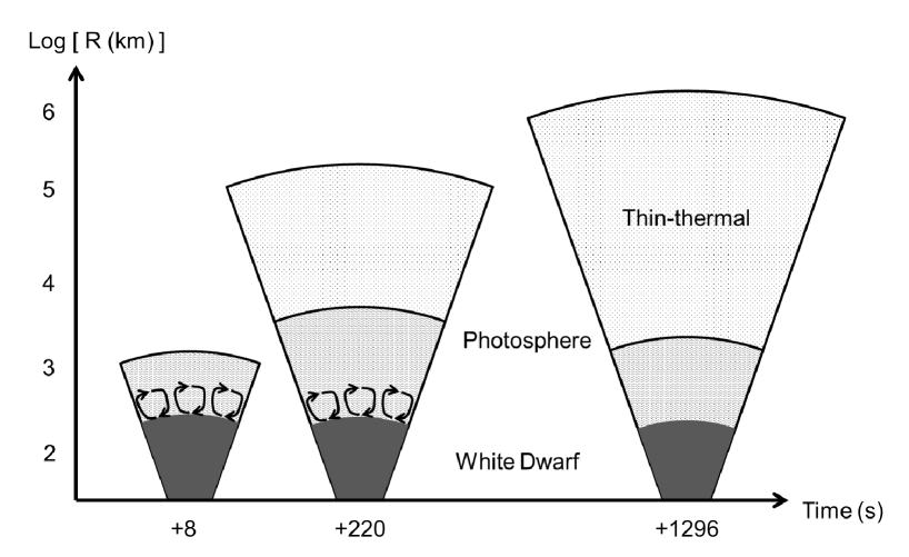
Figure 5: Schematic view of the ignition phase of the nova, MAXI J0158$-$744. The super-Eddington luminosity is produced by convection during the first $\sim 100$ s. The neon emission line at $+1296$ s was produced from the optically-thin thermal region filled with the ejecta dredged-up from the O-Ne WD.

5 Summary

Monitor of All-sky X-ray Image (MAXI) discovered an extraordinarily luminous soft X-ray transient, MAXI J0158$-$744, near the Small Magellanic Cloud (SMC) on 2011 November 11. This source is a binary system consisting of a white dwarf (WD) and a Be star at the distance of the SMC. MAXI detected it in three scans at $+8$ s, $+220$ s and $+1296$ s after the trigger time. The X-ray luminosity peaked on the second scan at $2\times 10^{40}$ erg s^-1 ($0.7-7.0$ keV), which is two orders of magnitude brighter than the Eddington luminosity of a solar mass object. The spectrum of the third scan showed a He-like neon emission, suggesting that the emission contains an optically-thin thermal component and the WD is a massive O-Ne WD. While the X-ray outburst could be considered as a kind of nova on the basis of the luminosity and the spectral evolutions, the huge peak luminosity and the rapid rise time ($<5.5\times 10^{3}$ s) are difficult to explain by shock-induced emission, accepted for optically-thin thermal emission in nova explosions observed so far. Instead, we propose the scenario that the X-ray outburst is the direct manifestation of the thermonuclear runaway process at the onset of the nova explosion, the so-called fireball phase. The super-Eddington X-ray outburst and the subsequent very early super-soft source phase indicate a small ejecta mass, implying the underlying WD is unusually massive near the Chandrasekhar limit, or possibly exceeding the limit.

References

- Anders & Grevesse (1989) Anders, E. & Grevesse, N. 1989, Geochimica et Cosmochimica Acta, 53, 197
- Band et al. (1993) Band, D. et al. 1993, ApJ, 413, 281
- Begelman (2001) Begelman, M. C. 2001, ApJ, 551, 897
- Bohlin, Savage & Drake (1978) Bohlin, R. C., Savage, B. D. & Drake, J. F. 1978, ApJ, 224, 132
- Burrows et al. (2005) Burrows, D. N. et al. 2005, Space Sci. Rev., 120, 165
- Carrera et al. (2008) Carrera, R. et al. 2008, AJ, 136, 1039
- Cash (1979) Cash, W. 1979, ApJ, 228, 939
- Das & Mukhopadhyay (2012) Das, U. & Mukhopadhyay, B. 2012, Phys. Rev. D, 86, 042001
- della Valle & Livio (1995) della Valle, M. & Livio, M. 1995, ApJ, 452, 704
- Dickey & Lockman (1990) Dickey, J. M. & Lockman, F. J. 1990, ARA&A, 28, 215
- Fujimoto (1982) Fujimoto, M. Y. 1982, ApJ, 257, 752
- Galloway et al. (2008) Galloway, D. K., Muno, M. P., Hartman, J. M., Psaltis, D. & Chakrabarty, D. 2008, ApJS, 179, 360
- Gehrels et al. (2004) Gehrels, N. et al. 2004, ApJ, 611, 1005
- Hachisu & Kato (2006) Hachisu, I. & Kato, M. 2006, ApJS, 167, 59
- Hachisu et al. (2012) Hachisu, I., Kato, M., Saio, H. & Nomoto, K. 2012, ApJ, 744, 69
- Henze et al. (2011) Henze, M. et al. 2011, A&A, 533, A52
- Hilditch, Howarth & Harries (2005) Hilditch, R. W., Howarth, I. D. & Harries, T. J. 2005, MNRAS, 357, 304
- Hiroi et al. (2011) Hiroi, K. et al. 2011, PASJ, 63, S677
- Kalberla et al. (2005) Kalberla, P. M. W. et al. 2005, A&A, 440, 775
- Kato & Hachisu (1994) Kato, M. & Hachisu, I. 1994, ApJ, 437, 802
- Kennea et al. (2011a) Kennea, J. A. et al. 2011, Proceedings of 4th International MAXI Workshop, arXiv:1101.6055
- Kennea et al. (2011b) Kennea, J. A. et al. 2011, Astron. Tel., 3758
- Kimura et al. (2011) Kimura, M. et al. 2011, Astron. Tel. 3756
- Kimura et al. (2012) Kimua, M. et al. 2012, PASJ, accepted (arXiv:1211.3737)
- Krautter (2008a) Krautter, J. 2008a, “The Super-soft Phase in Novae” in “RS Ophiuchi (2006) and the Recurrent Nova Phenomenon”, ASP Conference Series, vol. 401, p.139, ed. A. Evans, M. F. Bode, T. J. O’Brien, and M. J. Darnley, San Francisco: Astronomical Society of the Pacific.
- Krautter (2008b) Krautter, J. 2008b, “X-ray emission from classical novae in outburst” in “Classical Novae”, 2nd. edition, ed. M. Bode & A. Evans, Cambridge Univ. Press
- Li et al. (2012) Li, K. L. et al. 2012, ApJ, 761, 99, 13
- Matsuoka et al. (2009) Matsuoka, M. et al. 2009, PASJ, 61, 999
- Mewe, Gronenschild & van den Oord (1985) Mewe, R., Gronenschild, E. H. B. M. & van den Oord, G. H. J. 1985, A&A, 62, 197
- Mihara et al. (2011) Mihara, T. et al. 2011, PASJ, 63, S623
- Morii et al. (2011a) Morii, M. et al. 2011a, GRB Coordinates Network, Circular Service, 12555
- Morii et al. (2011b) Morii, M. et al. 2011b, PASJ, 63, S821
- Morrissey et al. (2005) Morrissey, P. et al. 2005, ApJ, 619, L7
- Nakahira et al. (2011) Nakahira, S. et al. 2012, PASJ, 64, 13
- Nauenberg (1972) Nauenberg, M. 1972, ApJ, 175, 417
- Negoro et al. (2010) Negoro, H. et al. 2010, Proceedings of a conference held October 4-8, 2009 in Sapporo, Japan. Ed. by Y. Mizumoto, K. Morita & M. Ohishi. ASP Conference Series, 434, San Francisco: Astronomical Society of the Pacific, 2010., p.127
- Nelson et al. (2012) Nelson, T., Donato, D., Mukai, K., Sokoloski, J. & Chomiuk, L. 2012, ApJ, 748, 16
- Nishiyama et al. (2007) Nishiyama, S. et al. 2007, ApJ, 658, 358
- Poole et al. (2008) Poole, T. S. et al. 2008, MNRAS, 383, 627
- Rauch et al. (2010) Rauch, T. et al. 2010, ApJ, 717, 363
- Roming et al. (2005) Roming, P. W. A. et al. 2005, Space Sci. Rev., 120, 95
- Rybicki & Lightman (1979) Rybicki, G. B. & Lightman, A. P. 1979, “Radiative processes in astrophysics”, John Wiley & Sons, Inc., U.S.
- Schlegel, Finkbeiner & Davis (1998) Schlegel, D. J., Finkbeiner, D. P. & Davis, M., 1998, ApJ, 500, 525
- Schwarz et al. (2011) Schwarz, G. J. et al. 2011, ApJS, 197, 31
- Sguera et al. (2006) Sguera, V. et al. 2006, ApJ, 646, 452
- Soderberg et al. (2008) Soderberg, A. M. et al. 2008, Nature, 453, 469
- Sokoloski et al. (2006) Sokoloski, J. L., Luna, G. J. M., Mukai, K. & Kenyon, S. J. 2006, Nature, 442, 276
- Starrfield et al. (1998) Starrfield, S. et al. 1998, MNRAS, 296, 502
- Starrfield, Iliadis & Hix (2008) Starrfield, S., Iliadis, C. & Hix, W. R. 2008, “Thermonuclear processes” in “Classical Novae”, 2nd. edition, ed. M. Bode & A. Evans, Cambridge Univ. Press
- Sugizaki et al. (2011) Sugizaki, M. et al. 2011, PASJ, 63, S635
- Tomida et al. (2011) Tomida, H. et al. 2011, PASJ, 63, 397
- Tsunemi et al. (2010) Tsunemi, H. et al. 2010, PASJ, 62, 1371
- van Rossum (2012) van Rossum, D. R. 2012, ApJ, 756, 43, 11
- Warner (1995) Warner, B. 1995, “Novae in Eruption” in “Cataclysmic Variable Stars”, Cambridge Univ. Press
- Warner (2008) Warner, B. 2008, “Properties of novae: an overview.” in “Classical Novae”, 2nd. edition, ed. M. Bode & A. Evans, Cambridge Univ. Press.
- Walter et al. (2004) Walter, F. M., Stringfellow, G. S., Sherry, W. H. & Field-Pollatou, A. 2004, AJ, 128, 1872
- Walter et al. (2012) Walter, F. M., Battisti, A., Towers, S. E., Bond, H. E. & Stringfellow, G. S. 2012, PASP, accepted (arXiv:1209.1583)
- Waters et al. (1988) Waters, L. B. F. M., van den Heuvel, E. P. J., Taylor, A. R., Habets, G. M. H. J. & Persi, P. 1988, A&A, 198, 200
- Woods & Thompson (2006) Woods, P. M. & Thompson, C. 2006, “Soft gamma repeaters and anomalous X-ray pulsars: magnetar candidates.” in “Compact stellar X-ray sources”. Ed. by W. Lewin & M. van der Klis. Cambridge Astrophysics Series, No. 39. Cambridge, UK: Cambridge University Press, 547
- Yoon & Langer (2004) Yoon, S.-C. & Langer, N. 2004, A&A, 419, 623
- Zorec et al. (2007) Zorec, J., Arias, M. L., Cidale, L. & Ringuelet, A. E. 2007, A&A, 470, 239