Processes that can be embedded
in a geometric Brownian motion

Abstract.

The main result is a counterpart of the theorem of Monroe [Ann. Probability 6 (1978) 42–56] for a geometric Brownian motion: A process is equivalent to a time change of a geometric Brownian motion if and only if it is a nonnegative supermartingale. We also provide a link between our main result and Monroe [Ann. Math. Statist. 43 (1972) 1293–1311]. This is based on the concept of a minimal stopping time, which is characterised in Monroe [Ann. Math. Statist. 43 (1972) 1293–1311] and Cox and Hobson [Probab. Theory Related Fields 135 (2006) 395–414] in the Brownian case. We finally suggest a sufficient condition for minimality (for the processes other than a Brownian motion) complementing the discussion in the aforementioned papers.

1. Introduction and Main Result

In his seminal paper Monroe [28] proves that a càdlàg process is equivalent to a finite time change of a Brownian motion if and only if it is a semimartingale. Here, the processes are said to be equivalent if they have the same law. We prove a counterpart of this result for a geometric Brownian motion:

Theorem 1.1.

(i) Let $X=(X_{s})_{s\geq 0}$ be a nonnegative supermartingale with $\mathsf{E}X_{0}\leq 1$. Then there exists a filtered probability space $(\Omega,\mathcal{F},(\mathcal{F}_{t})_{t\geq 0},\mathsf{P})$, an $(\mathcal{F}_{t},\mathsf{P})$-Brownian motion $W=(W_{t})$ and a $[0,\infty]$-valued $(\mathcal{F}_{t})$-time change $(T_{s})$ such that the processes $(X_{s})_{s\geq 0}$ and $(Z_{T_{s}})_{s\geq 0}$ have the same law, where $Z_{t}=e^{W_{t}-t/2}$, $t\geq 0$.

(ii) Conversely, for any $[0,\infty]$-valued $(\mathcal{F}_{t})$-time change $(T_{s})$, the process $(Z_{T_{s}})$ is a nonnegative $(\mathcal{F}_{T_{s}},\mathsf{P})$-supermartingale.

Part (ii) immediately follows from the optional sampling theorem for nonnegative supermartingales applied to $(Z_{t})$, so the task is to prove part (i).

We follow the usual convention of working with càdlàg processes. In particular, “supermartingale” means “càdlàg supermartingale”. Let us recall that a time change is a family $(T_{s})_{s\geq 0}$ of stopping times such that the maps $s\mapsto T_{s}$ are a.s. nondecreasing and right-continuous. In contrast to Monroe’s [28] setting the stopping times $T_{s}$ need not be finite here. This is natural in our setting because the nonnegative martingale $(Z_{t})$ has limit $Z_{\infty}\equiv 0$ and is closed as a supermartingale by this limit.

On the one hand, it is often helpful to know whether a random process can be considered as a time-changed process with a simple structure. In finance, the modelling approach based on time changes was, in fact, even inspired by Monroe’s theorem, see [2]. Nowadays this modelling approach is very popular in financial mathematics, see [6] and the references therein. On the other hand, Monroe’s theorem is one of the offsprings of the Skorokhod Embedding Problem (abbreviated below as the SEP). The latter was originally formulated and solved in [35] (English translation in [36]) and gave rise to a huge amount of literature. In [29] one finds a comprehensive survey of the state of the art to 2004, in particular, more than twenty different approaches to solve the SEP with the relations between them, different settings and generalisations as well as some other offsprings. Skorokhod’s motivation for the SEP was proving limit theorems (e.g. one can obtain the law of the iterated logarithm for random walks from that for a Brownian motion), but in recent years there appeared also other applications. The methodology based on Skorokhod embedding and pathwise inequalities proved to be important for finding model-independent bounds for option prices and robust hedging strategies. That gave rise to further research in this direction, which continues nowadays, see e.g. [21], [10], [14], [15], [16], [1], [8], [17], [18]. One finds more details and many further references in recent surveys on the SEP and its applications to robust pricing and hedging [22] and [30].

In spite of the generality of Monroe’s theorem, we cannot obtain Theorem 1.1 as its consequence (the reason is described in Section 3) and should therefore prove Theorem 1.1 independently. To prove it we proceed similarly to Monroe [28], although some technical details are elaborated differently, which is due to natural differences between the settings. In the first step, we consider the SEP for a geometric Brownian motion (i.e. embedding of a single random variable in a geometric Brownian motion). Different solutions to this problem (in fact, to the one for a Brownian motion with drift) were proposed in [20], [19], [33], [3], [5], and [4]. In Section 2.1, we suggest an alternative construction, which is, in our view, of interest in its own right. Also this construction will be convenient in Section 2.2. In the literature, there are already explicit embeddings in time-homogeneous diffusions, see [32], [12], [4], Section 9 in [29], Section 4.3 in [22] and the references therein. However, to the best of our knowledge, the construction that we present in Section 2.1 did not appear in the papers on the subject, although the ideas behind it are of course present in the literature. Most notably, our construction can be viewed as a rework of the original Skorokhod’s construction (see [36] or Section 3.12 in [22]) for the case of a geometric Brownian motion. In the second step, we embed discrete-time supermartingales in a geometric Brownian motion. Typically, if it is known how to embed one random variable, there is no problem to embed a discrete-time process. However, in our situation, this step turns out to be surprisingly technical. The reason is that the time change is allowed to take infinite value, see Section 2.2 for more details. In the third step, we justify a passage to the continuous-time limit. This part is closer to the corresponding part of the proof of Monroe’s theorem, and we, in fact, just refer to [28] at some point (see Section 2.3). In Section 3, we discuss some issues related to minimal stopping times for a Brownian motion, the concept studied in another Monroe’s paper [27] and taken on in many subsequent works on the SEP and its offsprings. In particular, we explain why Theorem 1.1 is not a consequence of [27] and [28] and provide in Theorem 3.5 an equivalent formulation of Theorem 1.1, which complements the discussion in [27]. For a Brownian motion, minimality is characterised in [27] and, in a more general situation, in [13]. In Section 4, we study minimal stopping times for other processes. Namely, in Theorem 4.2, we give a sufficient condition for minimality, which is new and complements the discussion of minimal stopping times for processes other than a Brownian motion in Section 8 in [29], Section 3.4 in [22] and Section 2.2 in [30]. We will see that Theorem 4.2 applies in many specific situations.

Let us finish the introduction by discussing the embedding in the process $\overline{Z}^{a,b}_{t}=e^{aW_{t}+bt}$, $t\geq 0$, where $a\neq 0$, $b\in\mathbb{R}$. First let $b\neq 0$, hence the (possibly infinite) limit $\overline{Z}^{a,b}_{\infty}:=\lim_{t\to\infty}\overline{Z}^{a,b}_{t}$ is well-defined, i.e. it is natural to consider $[0,\infty]$-valued time changes. Then Theorem 1.1 implies that a càdlàg process $\overline{X}$ is equivalent to a $[0,\infty]$-valued time change of $\overline{Z}^{a,b}$ if and only if $\overline{X}^{\lambda}$ is a nonnegative supermartingale with $\mathsf{E}\overline{X}_{0}^{\lambda}\leq 1$, where $\lambda=-\frac{2b}{a^{2}}$. Note that if $b>0$, then $\overline{X}$ is allowed to take value $+\infty$. Let now $b=0$. Since $\lim_{t\to\infty}\overline{Z}^{a,0}_{t}$ does not exist, it is now natural to consider only finite time changes. Then Monroe’s theorem implies that a càdlàg process $\overline{X}$ is equivalent to a finite time change of $\overline{Z}^{a,0}$ if and only if it is a strictly positive semimartingale.

2. Proof of Theorem 1.1

2.1. Embedding of a Single Random Variable

We will use the notation $\mu_{W}$ for the Wiener measure on $(C(\mathbb{R}_{+}),\mathcal{B}(C(\mathbb{R}_{+})))$ and $\mu_{L}$ for the Lebesgue measure on $([0,1],\mathcal{B}([0,1]))$. For some random variables $\xi$ and $\eta$, we write $\xi\sim\eta$ to express that $\xi$ and $\eta$ have the same law.

Lemma 2.1.

Let $\xi$ be a nonnegative random variable with $\mathsf{E}\xi\leq 1$. Consider the filtered probability space $(\Omega,\mathcal{F},(\mathcal{F}_{t})_{t\geq 0},\mathsf{P})$ with

$$\Omega=C(\mathbb{R}_{+})\times[0,1],\quad\mathcal{F}=\mathcal{B}(C(\mathbb{R}_{+}))\otimes\mathcal{B}([0,1]),\quad\mathsf{P}=\mu_{W}\times\mu_{L},$$

and $\mathcal{F}_{t}=\bigcap_{\varepsilon>0}\sigma(R,B_{s};s\in[0,t+\varepsilon])$, where the random variable $R$ and the process $B=(B_{t})$ on $\Omega$ are defined as follows: for $\omega=(x,r)$, $R(\omega):=r$, $B_{t}(\omega):=x(t)$. In particular, $R$ is $\mathcal{F}_{0}$-measurable and uniformly distributed on $[0,1]$, and $B$ is an $(\mathcal{F}_{t},\mathsf{P})$-Brownian motion. Then there exists a $[0,\infty]$-valued $(\mathcal{F}_{t})$-stopping time $\tau$ such that $\xi\sim Y_{\tau}$, where $Y_{t}=e^{B_{t}-t/2}$, $t\geq 0$.

Let us remark at this point that the converse, obviously, holds as well, i.e. a random variable can be embedded in a geometric Brownian motion if and only if it is nonnegative and its expectation is less than or equal to one.

Proof.

Let $F$ denote the distribution function of $\xi$ and let the quantile function $F^{-1}\colon[0,1]\to[0,+\infty]$ be defined as the right-continuous inverse of $F$, i.e. $F^{-1}(r)=\inf\{x\in\mathbb{R}_{+}\colon F(x)>r\}$; here and below $\inf\emptyset=+\infty$. It is well known that $F^{-1}(R)$ has the same distribution as $\xi$. Therefore, below we assume without loss of generality that $\xi=F^{-1}(R)$.

Let us set $h(r)=\int_{0}^{r}F^{-1}(s)\,ds$, $g(r)=r-h(r)$, $r\in[0,1]$. Then $h$ is a nondecreasing convex function on $[0,1]$, $h(0)=0$, $h(1)=\mathsf{E}\xi\leq 1$. If $h(1)<1$, the equation $g(x)=c$ for $0\leq c<g(1)$ has exactly one solution, say, $\theta=\theta(c)\in[0,1]$. For such $\theta$, we put $U(\theta)=F^{-1}(\theta)$, $V(\theta)=+\infty$. If $g(1)\leq c<g^{*}:=\max_{r\in[0,1]}g(r)$, the same equation has two solutions $\theta_{1}<\theta_{2}$ in $[0,1]$. For such $\theta_{1}$ and $\theta_{2}$, we put $U(\theta_{1})=U(\theta_{2})=F^{-1}(\theta_{1})$, $V(\theta_{1})=V(\theta_{2})=F^{-1}(\theta_{2})$. For $\theta\in[0,1]$ such that $g(\theta)=g^{*}$, we put $U(\theta)=V(\theta)=1$. We thus defined the functions $U\colon[0,1]\to[0,1]$ and $V\colon[0,1]\to[1,+\infty]$. Finally, let us introduce the random variables $\eta:=g(R)$, $\alpha:=U(R)$ and $\beta:=V(R)$. Note that $\alpha$ and $\beta$ are, in fact, functions of $\eta$. In Figure 1 we explain the structure of the random variables $\xi$, $\alpha$ and $\beta$ via the graphs of the functions $h$ and $g$.

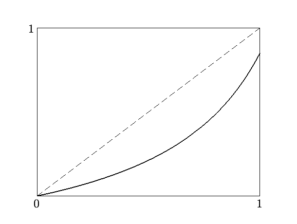
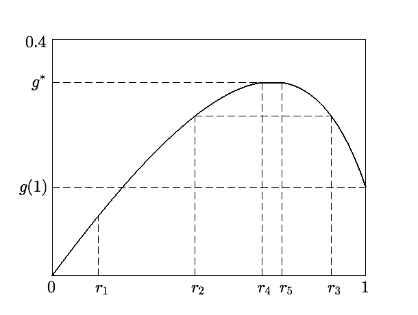
Figure 1. In the figure on the left, the solid line is the graph of the function $r\mapsto h(r)$, the dashed line is that of the identity function $r\mapsto r$. The relation with the structure of the random variable $\xi$ is explained by the formula $\xi=F^{-1}(R)=h^{\prime}_{+}(R)$, where $h^{\prime}_{+}$ denotes the right derivative of the convex function $h$. In the figure on the right, the solid line is the graph of the function $r\mapsto g(r)$. The structure of the random variables $\alpha$ and $\beta$ can be explained as follows: if $R=r_{1}$, then $\alpha=F^{-1}(r_{1})=\xi$ and $\beta=+\infty$; if $R\in\{r_{2},r_{3}\}$, then $\alpha=F^{-1}(r_{2})$ and $\beta=F^{-1}(r_{3})$; if $R\in[r_{4},r_{5}]$, then $\alpha=\beta=1$.

The key point of our construction is the following characterisation of the conditional law of $\xi$ given $\eta$:

(a) A.s. on the event $\{\eta<g(1)\}$ it is concentrated on the one-point set $\{\xi\}$ (note that $\xi$ is a function of $\eta$ on this event because $R$ and $\eta$ are in a one-to-one correspondence on $\{\eta<g(1)\}$);

(b) A.s. on the event $\{\eta\geq g(1)\}$ it is concentrated on the set $\{\alpha,\beta\}$ and, moreover,

(2.1) $$\mathsf{E}(\xi|\eta)=1\text{ a.s. on }\{\eta\geq g(1)\},$$

which determines the conditional law of $\xi$ given $\eta$ in a unique way.

To prove (2.1), it is sufficient to check that for any interval $(a,b)\subset[g(1),g^{*}]$, it follows $\mathsf{E}\xi 1_{\{\eta\in(a,b)\}}=\mathsf{P}\bigl{(}\eta\in(a,b)\bigr{)}$. We have $\{\eta\in(a,b)\}=\{g(R)\in(a,b)\}=\{R\in(r_{0},r_{1})\cup(r_{2},r_{3})\}$ with $g(r_{0})=g(r_{3})=a$ and $g(r_{1})=g(r_{2})=b$, therefore,

$$\mathsf{E}\xi 1_{\{\eta\in(a,b)\}} =\mathsf{E}F^{-1}(R)1_{\{g(R)\in(a,b)\}}=(h(r_{1})-h(r_{0}))+(h(r_{3})-h(r_{2}))$$

$$=(r_{1}-r_{0})+(r_{3}-r_{2})=\mathsf{P}\bigl{(}R\in(r_{0},r_{1})\cup(r_{2},r_{3})\bigr{)}=\mathsf{P}\bigl{(}\eta\in(a,b)\bigr{)}$$

(recall the definitions of the functions $g$ and $h$). The other statements in (a) and (b) above are clear.

Now we define $\tau$ by the formula

$$\tau=\inf\{t\in\mathbb{R}_{+}:Y_{t}\notin(\alpha,\beta)\}.$$

Since the random variables $\alpha$ and $\beta$ are $\mathcal{F}_{0}$-measurable, $\tau$ is an $(\mathcal{F}_{t})$-stopping time. Let us prove that the conditional law of $Y_{\tau}$ given $\eta$ admits the following characterisation:

(A) A.s. on the event $\{\eta<g(1)\}$ it is concentrated on the one-point set $\{\xi\}$;

(B) A.s. on the event $\{\eta\geq g(1)\}$ it is concentrated on the set $\{\alpha,\beta\}$ and, moreover,

(2.2) $$\mathsf{E}(Y_{\tau}|\eta)=1\text{ a.s. on }\{\eta\geq g(1)\}.$$

Indeed, if $\mathsf{P}(\eta<g(1))>0$, then on $\{\eta<g(1)\}$ it holds $\beta=\infty$ and, since $\lim_{t\to\infty}Y_{t}=0$ a.s., we have $Y_{\tau}=\alpha=F^{-1}(R)=\xi$ on this event (the case $\alpha=0$, where $\tau=\infty$, is included). The first statement in (B) is clear. It remains to check (2.2). Let us take $r\in[0,1]$ such that $g(r)\geq g(1)$. Since $V(r)<\infty$ for such $r$, the process $\big{(}Y(\cdot,r)_{t\wedge\tau(\cdot,r)}\big{)}$ is a bounded martingale on $C(\mathbb{R}_{+})$ with respect to the coordinate filtration and the Wiener measure $\mu_{W}$, i.e. $\int_{C(\mathbb{R}_{+})}Y(x,r)_{\tau(x,r)}\mu_{W}(dx)=1$, which means that $\mathsf{E}(Y_{\tau}|R)=1$ a.s. on $\{\eta\geq g(1)\}$. Statement (2.2) now follows by the tower property of conditional expectations.

Comparing (a), (b) and (A), (B) above we obtain that the conditional laws of $\xi$ and $Y_{\tau}$ given $\eta$ coincide. Hence, their unconditional laws coincide. This concludes the proof. ∎

Remark 2.2.

(i) At first glance it might seem tempting to prove Lemma 2.1 via a construction like Doob’s construction for embedding in a Brownian motion (see the paragraph following Problem I in Section 3). However, this does not work because $Y$ is transient. Namely, for the stopping time $\tau$ defined similarly to (3.1), we shall typically have $Y_{\tau}\neq f(Y_{1})\sim\xi$.

(ii) The proof of Lemma 2.1 provides an alternative solution to the Skorokhod embedding problem for a geometric Brownian motion. It is reminiscent of Hall’s solution [20], although qualitatively different from it. Both in [20] and in the proof above the stopping time is constructed as the hitting time of two levels, $\alpha$ and $\beta$, that are obtained via a randomization. However, these randomizations are very different. For instance, if the law of $\xi$ has no atoms, then $\beta$ in our construction is always a deterministic function of $\alpha$, while in [20] the random vector $(\alpha,\beta)$ is “genuinely two-dimensional”, i.e. the conditional distribution of $\beta$ given $\alpha$ is nondegenerate.

(iii) The construction in the proof of Lemma 2.1 appeared earlier in statistical context in [9] in the proof that each binary experiment is equivalent to a mixture of strictly ordered simple binary experiments. Here we tailored the construction to our situation and found a short proof via (2.1).

(iv) Other solutions to the SEP for a geometric Brownian motion or, equivalently, for a Brownian motion with drift were obtained in a number of papers mentioned in the introduction. One more way to construct required embeddings is to reduce the problem to the SEP for a Brownian motion and non-centred target distributions via change of time, see the explanation in Section 3. Then one can use the solution proposed by Cox [11] or just run the Brownian motion until it hits the mean of the distribution and then use a solution in the centred case.

(v) For the sequel, let us remark that the levels $\alpha$ and $\beta$ in the proof of Lemma 2.1 depend on an external uniformly distributed on $[0,1]$ random variable $R$ and on the distribution $F$ we want to embed: with a slight abuse of notation we will write $\alpha=\alpha(F,R)$, $\beta=\beta(F,R)$ (recall Figure 1 and observe that the functions $h$ and $g$ are constructed via $F$).

2.2. Embedding of a Discrete-Time Supermartingale.

Using Lemma 2.1 we now embed a nonnegative discrete-time supermartingale in a geometric Brownian motion. Let $\mathbb{N}_{0}:=\mathbb{N}\cup\{0\}$. We will also use the notation $\operatorname{Law}_{\mathsf{P}}(\xi)$ (resp. $\operatorname{Law}_{\mathsf{P}}(\xi|\eta)$ or $\operatorname{Law}_{\mathsf{P}}(\xi|\mathcal{G})$) for the law of $\xi$ under $\mathsf{P}$ (resp. for the conditional law of $\xi$ given $\eta$ or given $\mathcal{G}$ under $\mathsf{P}$) whenever $\xi$ and $\eta$ are random elements and $\mathcal{G}$ is a sub-$\sigma$-field on some probability space $(\Omega,\mathcal{F},\mathsf{P})$.

Lemma 2.3.

Let $X=(X_{n})_{n\in\mathbb{N}_{0}}$ be a nonnegative supermartingale with $\mathsf{E}X_{0}\leq 1$. Consider the filtered probability space $(\Omega,\mathcal{F},(\mathcal{F}_{t})_{t\geq 0},\mathsf{P})$ with

$$\Omega=C(\mathbb{R}_{+})\times[0,1]^{\mathbb{N}_{0}},\quad\mathcal{F}=\mathcal{B}(C(\mathbb{R}_{+}))\otimes\mathcal{B}([0,1])^{\otimes\mathbb{N}_{0}},\quad\mathsf{P}=\mu_{W}\times\mu_{L}^{\mathbb{N}_{0}},$$

and $\mathcal{F}_{t}=\bigcap_{\varepsilon>0}\sigma(R_{n},B_{s};n\in\mathbb{N}_{0},s\in[0,t+\varepsilon])$, where the random variables $R_{n}$ and the process $B=(B_{t})$ on $\Omega$ are defined as follows: for $\omega=(x,r_{0},r_{1},\ldots)$, $R_{n}(\omega):=r_{n}$, $B_{t}(\omega):=x(t)$. In particular, $R_{n}$, $n\in\mathbb{N}_{0}$, are independent $\mathcal{F}_{0}$-measurable uniformly distributed on $[0,1]$ random variables, and $B$ is an $(\mathcal{F}_{t},\mathsf{P})$-Brownian motion (note that independence of $B$ and $(R_{n})$ is included in this statement). Then there exists a nondecreasing family $(\tau_{n})$ of $[0,\infty]$-valued $(\mathcal{F}_{t})$-stopping times such that the processes $(X_{n})$ and $(Y_{\tau_{n}})$ have the same law, where $Y_{t}=e^{B_{t}-t/2}$, $t\geq 0$.

Proof.

Let $F_{0}$ denote the distribution function of $X_{0}$. Consider the $(\mathcal{F}_{t})$-stopping time

$$\tau_{0}=\inf\big{\{}t\in\mathbb{R}_{+}:Y_{t}\notin\big{(}\alpha(F_{0},R_{0}),\beta(F_{0},R_{0})\big{)}\big{\}},$$

where the notations $\alpha(F_{0},R_{0})$ and $\beta(F_{0},R_{0})$ are introduced in Remark 2.2 (v). By Lemma 2.1, the random variables $X_{0}$ and $Y_{\tau_{0}}$ have the same law. For the sequel let us also observe that the family $(R_{n})_{n\geq 1}$ is independent of $\sigma(\tau_{0},Y_{t};\,t\geq 0)$ under $\mathsf{P}$.

We proceed by induction. The induction hypothesis is as follows. For some $k\in\mathbb{N}_{0}$, we constructed a nondecreasing family $(\tau_{n})_{0\leq n\leq k}$ of $(\mathcal{F}_{t})$-stopping times such that

(2.3) $$\operatorname{Law}_{\mathsf{Pr}}(X_{0},\ldots,X_{k})=\operatorname{Law}_{\mathsf{P}}(Y_{\tau_{0}},\ldots,Y_{\tau_{k}})$$

(here and below $\mathsf{Pr}$ denotes the probability measure on the space, where the sequence $(X_{n})$ is defined) and that

(2.4) $$(R_{n})_{n\geq k+1}\text{ is independent of }\sigma\big{(}Y_{t},\tau_{n};\,t\geq 0,0\leq n\leq k\big{)}\text{ under }\mathsf{P}.$$

We need to construct an $(\mathcal{F}_{t})$-stopping time $\tau_{k+1}\geq\tau_{k}$ such that (2.3) and (2.4) hold with $k$ replaced by $k+1$.

In what follows we will work with the random variables like $\frac{X_{k+1}}{X_{k}}$ employing the convention $\frac{0}{0}:=1$ (note that $X_{k+1}=0$ $\mathsf{Pr}$-a.s. on the set $\{X_{k}=0\}$ because $(X_{n})$ is a nonnegative supermartingale). Let us remark that $\mathsf{E}_{\mathsf{Pr}}\big{(}\frac{X_{k+1}}{X_{k}}\big{|}X_{0},\ldots,X_{k}\big{)}\leq 1$ $\mathsf{Pr}$-a.s. The idea is now to embed $\operatorname{Law}_{\mathsf{Pr}}\big{(}\frac{X_{k+1}}{X_{k}}\big{|}X_{0},\ldots,X_{k}\big{)}$ via Lemma 2.1 in the geometric Brownian motion $({Y_{t+\tau_{k}}}/{Y_{\tau_{k}}})$, but this requires some additional technical work because $\tau_{k}$ may take infinite value.

Let us consider the regular conditional distribution function $F_{k+1}=(F_{k+1}(x|x_{0},\ldots,x_{k}))_{x,x_{0},\ldots,x_{k}\in\mathbb{R}_{+}}$ for the random variable $\frac{X_{k+1}}{X_{k}}$ given $X_{0},\ldots,X_{k}$. Namely, for each $x_{0},\ldots,x_{k}\in\mathbb{R}_{+}$, $F_{k+1}(\cdot|x_{0},\ldots,x_{k})$ is a distribution function of a probability measure on $\mathbb{R}_{+}$; for each $x\in\mathbb{R}_{+}$, $F_{k+1}(x|\cdot)$ is a Borel function on $\mathbb{R}_{+}^{k+1}$, and the random variable $F_{k+1}(x|X_{0},\ldots,X_{k})$ is a version of the conditional probability $\mathsf{Pr}\big{(}\frac{X_{k+1}}{X_{k}}\leq x\big{|}X_{0},\ldots,X_{k}\big{)}$. We define $\tau_{k+1}$ by the formula

$$\tau_{k+1}=\tau_{k}+\inf\left\{t\in\mathbb{R}_{+}:\frac{Y_{t+\tau_{k}}}{Y_{\tau_{k}}}\notin\big{(}\alpha(F_{k+1}(\cdot|Y_{\tau_{0}},\ldots,Y_{\tau_{k}}),R_{k+1}),\beta(F_{k+1}(\cdot|Y_{\tau_{0}},\ldots,Y_{\tau_{k}}),R_{k+1})\big{)}\right\}$$

($\tau_{k+1}:=\infty$ on the event $\{\tau_{k}=\infty\}$), which is an $(\mathcal{F}_{t})$-stopping time because $R_{k+1}$ is $\mathcal{F}_{0}$-measurable and $F_{k+1}(\cdot|Y_{\tau_{0}},\ldots,Y_{\tau_{k}})$ is known at time $\tau_{k}$. Let us note that (2.4) with $k$ replaced by $k+1$ follows from the formula for $\tau_{k+1}$, (2.4) and the fact that $R_{k+1},R_{k+2},\ldots$ are independent under $\mathsf{P}$. It remains to prove that

(2.5) $$\operatorname{Law}_{\mathsf{Pr}}(X_{0},\ldots,X_{k+1})=\operatorname{Law}_{\mathsf{P}}(Y_{\tau_{0}},\ldots,Y_{\tau_{k+1}}).$$

If $\mathsf{P}(\tau_{k}=\infty)=1$ (equivalently, $\mathsf{Pr}(X_{k}=0)=1$), then $Y_{\tau_{k+1}}=0$ $\mathsf{P}$-a.s. and $X_{k+1}=0$ $\mathsf{Pr}$-a.s., so (2.5) follows from (2.3). Below we assume that $\mathsf{P}(\tau_{k}<\infty)>0$. Let us introduce the probability measure $\mathsf{Q}$ on $(\Omega,\mathcal{F})$ by the formula

$$\mathsf{Q}(\cdot):=\mathsf{P}(\cdot|\tau_{k}<\infty).$$

We will use the notation $\mathcal{G}:=\sigma(Y_{\tau_{0}},\ldots,Y_{\tau_{k}})$. One can easily check that, for any nonnegative random variable $Z$, we have

(2.6) $$\mathsf{E}_{\mathsf{Q}}(Z|\mathcal{G})=\mathsf{E}_{\mathsf{P}}(Z|\mathcal{G})\quad\mathsf{P}\text{-a.s. on }\{\tau_{k}<\infty\}$$

(note that $\mathsf{P}$-a.s. we have $\{\tau_{k}<\infty\}=\{Y_{\tau_{k}}>0\}\in\mathcal{G}$) or, equivalently,

(2.7) $$\mathsf{E}_{\mathsf{Q}}(Z|\mathcal{G})=\mathsf{E}_{\mathsf{P}}(Z|\mathcal{G})\quad\mathsf{Q}\text{-a.s.\phantom{ on }}\phantom{\{\tau_{k}<\infty\}}$$

In fact, the identities (2.6) and (2.7) hold even conditionally on $\mathcal{F}_{\tau_{k}}$. It follows from (2.7) and (2.4) that, for $x\in[0,1]$, $\mathsf{Q}$-a.s. we have

(2.8) $$\mathsf{Q}(R_{k+1}\leq x|\mathcal{G})=\mathsf{P}(R_{k+1}\leq x|\mathcal{G})=\mathsf{P}(R_{k+1}\leq x)=x,$$

i.e. under $\mathsf{Q}$ conditionally on $\mathcal{G}$ the random variable $R_{k+1}$ is uniformly distributed on $[0,1]$. Let now $A\in\mathcal{G}$ and $B=\{R_{k+1}\leq x\}$. Then, by (2.8),

$$\mathsf{Q}(A\cap B)=\mathsf{E}_{\mathsf{Q}}\left[1_{A}\mathsf{Q}(B|\mathcal{G})\right]=\mathsf{E}_{\mathsf{Q}}\left[1_{A}\mathsf{Q}(B)\right]=\mathsf{Q}(A)\mathsf{Q}(B),$$

i.e. $\mathcal{G}$ and $R_{k+1}$ are independent under $\mathsf{Q}$. One can deduce from the strong Markov property of Brownian motion (e.g. in the form [34, Ch. III, Th. 3.1]) that under $\mathsf{Q}$ the process $(Y_{t+\tau_{k}}/Y_{\tau_{k}})$ is a geometric Brownian motion independent of $\mathcal{F}_{\tau_{k}}$. Since $\mathcal{G}\subset\mathcal{F}_{\tau_{k}}$ and $R_{k+1}$ is $\mathcal{F}_{\tau_{k}}$-measurable (even $\mathcal{F}_{0}$-measurable), we get

(2.9) $$\left({Y_{t+\tau_{k}}}/{Y_{\tau_{k}}}\right)_{t\geq 0},\;\mathcal{G}\text{ and }R_{k+1}\text{ are independent under }\mathsf{Q}.$$

Summarising, we have:

1. Under $\mathsf{Q}$ conditionally on $\mathcal{G}$ the process $(Y_{t+\tau_{k}}/Y_{\tau_{k}})$ is a geometric Brownian motion.

2. Under $\mathsf{Q}$ conditionally on $\mathcal{G}$ the random variable $R_{k+1}$ is uniformly distributed on $[0,1]$.

3. Under $\mathsf{Q}$ conditionally on $\mathcal{G}$ the process $(Y_{t+\tau_{k}}/Y_{\tau_{k}})$ and the random variable $R_{k+1}$ are independent (this follows from (2.9)).

Therefore, by Lemma 2.1 applied under $\mathsf{Q}$ conditionally on $\mathcal{G}$, for any $x\in\mathbb{R}_{+}$, $\mathsf{Q}$-a.s. it holds

$$\mathsf{Q}\left(\left.\frac{Y_{\tau_{k+1}}}{Y_{\tau_{k}}}\leq x\right|\mathcal{G}\right)=F_{k+1}(x|Y_{\tau_{0}},\ldots,Y_{\tau_{k}}).$$

By (2.6), $\mathsf{P}$-a.s. on $\{\tau_{k}<\infty\}$ it holds

(2.10) $$\mathsf{P}\left(\left.\frac{Y_{\tau_{k+1}}}{Y_{\tau_{k}}}\leq x\right|\mathcal{G}\right)=F_{k+1}(x|Y_{\tau_{0}},\ldots,Y_{\tau_{k}}).$$

But $\mathsf{P}$-a.s. on $\{\tau_{k}=\infty\}(\equiv\{Y_{\tau_{k}}=0\})$ we have $Y_{\tau_{k+1}}=0$, i.e. the left-hand side of (2.10) is then $1_{\{x\geq 1\}}$, which coincides with the right-hand side of (2.10) on this event. Thus, (2.10) holds $\mathsf{P}$-a.s. on $\Omega$ (not only on $\{\tau_{k}<\infty\}$). Since $x\in\mathbb{R}_{+}$ is arbitrary, this implies that $F_{k+1}(\cdot|Y_{\tau_{0}},\ldots,Y_{\tau_{k}})$ is a version of the regular conditional distribution function (under $\mathsf{P}$) of $Y_{\tau_{k+1}}/Y_{\tau_{k}}$ given $Y_{\tau_{0}},\ldots,Y_{\tau_{k}}$. Together with (2.3) and the definition of $F_{k+1}$ this implies (2.5). The induction step is proved.

Thus, we can construct a nondecreasing family $(\tau_{n})$ of $(\mathcal{F}_{t})$-stopping times such that the discrete-time processes $(X_{n})$ and $(Y_{\tau_{n}})$ have the same finite-dimensional distributions. This completes the proof of the lemma. ∎

2.3. Continuous-Time Limit.

Let us proceed with the proof of Theorem 1.1. We are now given a continuous-time nonnegative supermartingale $(X_{s})$ with $\mathsf{E}X_{0}\leq 1$. For each $n\in\mathbb{N}$, let us consider the piecewise constant nonnegative supermartingale $(X^{n}_{s})=\big{(}X_{2^{-n}\lfloor 2^{n}s\rfloor}\big{)}$. By Lemma 2.3, there exists a geometric Brownian motion $(Y^{n}_{t})$ and a (piecewise constant) time change $(T^{n}_{s})$ on some filtered probability space $(\Omega^{n},\mathcal{F}^{n},(\mathcal{F}^{n}_{t}),\mathsf{P}^{n})$ such that the processes $(X^{n}_{s})$ and $(Y^{n}_{T^{n}_{s}})$ have the same law. Without loss of generality we assume that $\lim_{t\to\infty}Y^{n}_{t}(\omega_{n})=0$ for all $\omega_{n}\in\Omega^{n}$ and set $Y^{n}_{\infty}(\omega_{n}):=0$ for all $\omega_{n}\in\Omega^{n}$.

Let $C([0,\infty])$ be the space of all continuous functions $z\colon[0,\infty]\to\mathbb{R}$ with the sup-norm, and let $\mathcal{A}$ be the set of all non-decreasing right-continuous functions $a\colon[0,\infty)\to[0,\infty]$. Define a metric $\rho$ on $\mathcal{A}$ by $\rho(a_{1},a_{2})=d(\hat{a}_{1},\hat{a}_{2})$, where $\hat{a}_{i}=\frac{a_{i}}{1+a_{i}}$ and

$$d(b_{1},b_{2})=\sum_{k=1}^{\infty}2^{-k}\int_{0}^{k}|b_{1}(t)-b_{2}(t)|dt.$$

It is easy to check that the convergence in the metric $d$ in the space $\hat{\mathcal{A}}$ of all non-decreasing right-continuous functions $b\colon[0,\infty)\to[0,1]$ is equivalent to the pointwise convergence for every point at which the limiting function is continuous. By Helly’s theorem, $(\hat{\mathcal{A}},d)$ is a compact. Hence, $(\mathcal{A},\rho)$ is a compact.

Put $\Omega=C([0,\infty])\times\mathcal{A}$, $\mathcal{F}=\mathcal{B}(C([0,\infty]))\otimes\mathcal{B}(\mathcal{A})$. The space $\Omega$ with the product topology is a complete separable metric space. We define the measurable mapping $f_{n}\colon\Omega^{n}\to\Omega$ by

$$f_{n}(\omega_{n})=(Y^{n}(\omega_{n}),T^{n}(\omega_{n})).$$

Let $\mathsf{Q}^{n}$ be the image of $\mathsf{P}^{n}$ under $f_{n}$. First, we show that the sequence $\mathsf{Q}_{n}$ of probability measures on $(\Omega,\mathcal{F})$ is tight. It is sufficient to check that the projections of $\mathsf{Q}^{n}$ on $C([0,\infty])$ and on $\mathcal{A}$ are tight. The projection of $\mathsf{Q}^{n}$ on $C([0,\infty])$ is the law of a geometric Brownian motion and does not depend on $n$, which implies the tightness of the projections on $C([0,\infty])$. The tightness of projections on $\mathcal{A}$ follows from the compactness of $\mathcal{A}$. Thus, the sequence $\mathsf{Q}^{n}$ is tight. Now we define $\mathsf{P}$ as an accumulation point of this sequence. It is evident that the process $(Z_{t})_{t\in\mathbb{R}_{+}}$ on $\Omega$ defined by $Z_{t}(z,a)=z(t)$ is a (standard) geometric Brownian motion under $\mathsf{P}$: namely, the process $(W_{t})_{t\in\mathbb{R}_{+}}$ with $W_{t}=\log Z_{t}+t/2$, which is well-defined under $\mathsf{P}$, is a Brownian motion under $\mathsf{P}$.

Define the process $(T_{s})_{s\in\mathbb{R}_{+}}$ on $\Omega$ by $T_{s}(z,a)=a(s)$ and consider the minimal right-continuous filtration $(\mathcal{F}_{t})_{t\in\mathbb{R}_{+}}$ on $\Omega$ with respect to which $(Z_{t})$ is adapted and $(T_{s})$ is a time change, i.e.

$$\mathcal{F}_{t}=\bigcap_{\varepsilon>0}\sigma\big{(}Z_{u},\{T_{s}\leq v\}\colon u,v\in[0,t+\varepsilon],s\in\mathbb{R}_{+}\big{)}.$$

The remaining steps of the proof are to show that:

1. The process $(Z_{T_{s}})$ has the same law under $\mathsf{P}$ as $(X_{s})$.

2. The process $(W_{t})$ is an $(\mathcal{F}_{t},\mathsf{P})$-Brownian motion, i.e. $W_{t}-W_{s}$ is independent of $\mathcal{F}_{s}$ under $\mathsf{P}$ for any $s<t$, $s,t\in\mathbb{R}_{+}$.

These two steps are proved similarly to the corresponding steps in the proof of Theorem 2 in [28] with obvious changes.

One can also give an alternative proof using a version of Theorem (3.2) in [7]. The idea is to introduce a kind of stable topology on $\Omega$ such that (2) remains true after passing to the limit; however, then the compactness is a nontrivial issue.

3. SEP, Minimality and Embedding of Processes

3.1. Classical SEP and Minimal Stopping Times

We start with a few remarks on the evolution of the formulation of the embedding problem for a Brownian motion.

Problem I (Embedding in a Brownian motion, naive formulation).

Given: a real-valued random variable $\xi$.
To find: a filtered probability space $(\Omega,\mathcal{F},(\mathcal{F}_{t})_{t\geq 0},\mathsf{P})$, an $(\mathcal{F}_{t},\mathsf{P})$-Brownian motion $B=(B_{t})$ and a finite $(\mathcal{F}_{t})$-stopping time $\tau$ such that $B_{\tau}\sim\xi$.

Problem I admits the following trivial solution. Let $f\colon\mathbb{R}\to\mathbb{R}$ be a function such that $f(B_{1})\sim\xi$. Then, with

(3.1) $$\tau:=\inf\{t\geq 1:B_{t}=f(B_{1})\},$$

due to recurrence of a Brownian motion, we have $B_{\tau}=f(B_{1})\sim\xi$. This solution is attributed to Doob (see the discussion in Section 2.3 in [29] or Section 3.2 in [22]) and is intended to show that without additional requirements the problem is trivial.

Therefore, the original formulation of the SEP contains some restrictions:

Problem II (SEP, Skorokhod [35] and [36]).

Given: a real-valued random variable $\xi$ with $\mathsf{E}\xi=0$ and $\mathsf{E}\xi^{2}<\infty$.
To find: a filtered probability space $(\Omega,\mathcal{F},(\mathcal{F}_{t})_{t\geq 0},\mathsf{P})$, an $(\mathcal{F}_{t},\mathsf{P})$-Brownian motion $B=(B_{t})$ and an $(\mathcal{F}_{t})$-stopping time $\tau$ with $\mathsf{E}\tau<\infty$ such that $B_{\tau}\sim\xi$.

Note that the stopping time $\tau$ of (3.1) is excluded because, for this stopping time, $\mathsf{E}\tau=\infty$ (unless $f$ is the identity function, which is only possible when $\xi\sim N(0,1)$). Let us further note that $\mathsf{E}\tau<\infty$ implies $\mathsf{E}B_{\tau}=0$ and $\mathsf{E}B_{\tau}^{2}=\mathsf{E}\tau$, hence we need to assume $\mathsf{E}\xi=0$ and $\mathsf{E}\xi^{2}<\infty$ in the formulation when we have the requirement $\mathsf{E}\tau<\infty$. However, these assumptions ($\mathsf{E}\xi=0$ and $\mathsf{E}\xi^{2}<\infty$) constitute the drawback of the formulation in Problem II. For example, the stopping times in the original Skorokhod’s construction (see [35] and [36]) require from $\xi$ only to have a finite mean, but, as we have just seen, unless we assume a finite variance, it is no longer clear how to select “good” stopping times.

A very natural way to select “good” stopping times is to require them to be minimal (instead of requiring $\mathsf{E}\tau<\infty$) in the following sense. A finite stopping time $\tau$ is said to be minimal if, for a stopping time $\sigma$, $\sigma\leq\tau$ and $B_{\sigma}\sim B_{\tau}$ imply $\sigma=\tau$ a.s. In the context of the SEP, this was suggested in [27] (such a concept of minimality is attributed by Monroe [27] to Doob) and taken on in many subsequent works on the SEP. In particular, for centred target distributions, minimality is characterised in [27] as follows.

Theorem 3.1 (Monroe [27]).

Let $\tau$ be a finite stopping time such that $\mathsf{E}B_{\tau}=0$. Then $\tau$ is minimal if and only if the process $(B_{t\wedge\tau})_{t\geq 0}$ is uniformly integrable.

This characterisation proved to be very useful. We will also need it below. Let us further remark that minimality for non-centred target distributions was characterised in [13], in particular, Theorem 3.1 was generalised for $\mathsf{E}|B_{\tau}|<\infty$. See also Section 8 in [29], Sections 3.4 and 4.2 in [22] as well as Section 2.2 in [30] for a further discussion of minimality.

Summarising, [27] and [13] inspire the following formulation of the SEP:

Problem III (SEP, Monroe [27], Cox and Hobson [13]).

Given: a real-valued random variable $\xi$.
To find: a filtered probability space $(\Omega,\mathcal{F},(\mathcal{F}_{t})_{t\geq 0},\mathsf{P})$, an $(\mathcal{F}_{t},\mathsf{P})$-Brownian motion $B=(B_{t})$ and a minimal $(\mathcal{F}_{t})$-stopping time $\tau$ such that $B_{\tau}\sim\xi$.

Let us note that Problem III is more general than Problem II in the sense that each solution of Problem II is a solution of Problem III (if $\sigma\leq\tau$ are solutions of Problem II, then $\mathsf{E}\tau=\mathsf{E}\sigma=\mathsf{E}\xi^{2}<\infty$, i.e. $\sigma=\tau$ a.s., hence $\tau$ is minimal), but we do not assume $\mathsf{E}\xi=0$ and $\mathsf{E}\xi^{2}<\infty$ any longer.

3.2. Embedding of Processes

Here we explain why Theorem 1.1 is not a consequence of [27] and [28]. In fact, what can be inferred directly from Monroe’s results is only the following (weaker) statement.

Proposition 3.2.

Let $X=(X_{s})_{s\geq 0}$ be a nonnegative martingale with $\mathsf{E}X_{0}=1$. Then there exists a filtered probability space $(\Omega,\mathcal{F},(\mathcal{F}_{t})_{t\geq 0},\mathsf{P})$, an $(\mathcal{F}_{t},\mathsf{P})$-Brownian motion $W=(W_{t})$ and a $[0,\infty]$-valued $(\mathcal{F}_{t})$-time change $(T_{s})$ such that the processes $(X_{s})_{s\geq 0}$ and $(Z_{T_{s}})_{s\geq 0}$ have the same law, where $Z_{t}=e^{W_{t}-t/2}$, $t\geq 0$.

Let us remark that nonnegative supermartingales $(X_{s})$ with $\mathsf{E}X_{0}\leq 1$ (see Theorem 1.1 (i)) is an important class of processes, which naturally appears in different branches of stochastics such as financial mathematics or sequential analysis. As for financial mathematics, so-called supermartingale deflators appear naturally as an extension of the class of the density processes of equivalent martingale measures. In particular, existence of a strictly positive supermartingale deflator is a weaker assumption than existence of equivalent (local) martingale measure and is equivalent to some form of absence of arbitrage, see [23]. Even if an equivalent local martingale measure exists, it is necessary to use supermartingale deflators in the utility maximization problem, see [26]. As for sequential analysis, let us, for instance, note that given two probability measures $\mathsf{P}$ and $\mathsf{Q}$ on a filtered space $(\Omega,\mathcal{F},(\mathcal{F}_{t}))$ the generalised density process $(\frac{d\mathsf{Q}_{t}}{d\mathsf{P}_{t}})$ is, in general, only a supermartingale under $\mathsf{P}$ (a martingale only when $\mathsf{Q}$ is locally absolutely continuous with respect to $\mathsf{P}$). Thus, it is really better to have Theorem 1.1 than just Proposition 3.2.

Turning to the discussion of the relations with Monroe’s results, let us first recall that both in [27] and in [28] the question is treated of whether a process is equivalent to a time-changed Brownian motion. The difference is that, in [27], only finite time changes consisting of minimal stopping times, while in [28], all finite time changes are considered. Therefore, the results are very different:

Theorem 3.3 (Monroe [27]).

Let $M=(M_{s})_{s\geq 0}$ be a martingale. Then there is a filtered probability space $(\Omega,\mathcal{F},(\mathcal{F}_{t})_{t\geq 0},\mathsf{P})$, an $(\mathcal{F}_{t},\mathsf{P})$-Brownian motion $W=(W_{t})$ and a finite $(\mathcal{F}_{t})$-time change $(T_{s})$ such that all stopping times $T_{s}$ are minimal and the processes $(M_{s})$ and $(W_{T_{s}})$ have the same law.

Theorem 3.4 (Monroe [28]).

A càdlàg process $X=(X_{s})_{s\geq 0}$ is a semimartingale if and only if there is a filtered probability space $(\Omega,\mathcal{F},(\mathcal{F}_{t})_{t\geq 0},\mathsf{P})$, an $(\mathcal{F}_{t},\mathsf{P})$-Brownian motion $W=(W_{t})$ and a finite $(\mathcal{F}_{t})$-time change $(T_{s})$ such that the processes $(X_{s})$ and $(W_{T_{s}})$ have the same law.

We now know what kind of processes can be viewed as time changes of a Brownian motion (Theorems 3.3 and 3.4), while we are interested in understanding of what kind of processes can be viewed as time changes of the geometric Brownian motion $Z=(Z_{t})$ of Theorem 1.1 (i). The idea is first to change time in $Z$ in order to get a Brownian motion starting from one (to which we then want to apply Monroe’s results), but it is only possible to obtain a Brownian motion absorbed at zero. More precisely, with $A_{t}:=[Z,Z]_{t}=\int_{0}^{t}Z_{r}^{2}\,dr$, we define the time change $\tau_{u}:=\inf\{r\geq 0:A_{r}>u\}$ and set

(3.2) $$B^{0}_{u}:=Z_{\tau_{u}},\quad u\geq 0.$$

Note that $A_{\infty}<\infty$ a.s. and that $(\tau_{u})$ is strictly increasing on $[0,A_{\infty})$ and is equal to $+\infty$ on $[A_{\infty},\infty)$. We have: $B^{0}=(B^{0}_{u})_{u\geq 0}$ is a Brownian motion absorbed at zero with $B^{0}_{0}=1$ (see [34, Ch. V, § 1]). Now the idea is: if we can embed a process $X$ in $B^{0}$ in the sense that $(X_{s})$ and $(B^{0}_{T_{s}})$ have the same law for some time change $(T_{s})$, then we can embed $X$ in $Z$ via the time change $(\tau_{T_{s}})$ (see (3.2)). At this point Theorem 3.3 turns out to be very useful and gives us Proposition 3.2. Namely, let $X$ be a nonnegative martingale with $\mathsf{E}X_{0}=1$. Applying Theorem 3.3 to the martingale $X-1$ we get that $(X_{s})$ has the same law as $(Y_{T_{s}})$ for some Brownian motion $Y$ starting from one and a time change $(T_{s})$ such that all stopping times $T_{s}$ are minimal. By Theorem 3.1, for each $s\geq 0$, the process $(Y_{u\wedge T_{s}})_{u\geq 0}$ is uniformly integrable. (The condition $\mathsf{E}B_{\tau}=0$ in Theorem 3.1 takes here the form $\mathsf{E}Y_{T_{s}}=1$ because $Y$ starts from one. This is fulfilled because $X$ is a martingale.) Since $X_{s}\geq 0$ a.s., we have $Y_{T_{s}}\geq 0$ a.s., hence the uniformly integrable martingale $(Y_{u\wedge T_{s}})_{u\geq 0}$ is nonnegative, which implies

$$T_{s}\leq H^{Y}_{0}:=\inf\{u\geq 0:Y_{u}=0\}\quad\text{a.s.}$$

Therefore, $Y_{T_{s}}=Y^{0}_{T_{s}}$ a.s. for all $s\geq 0$, where $Y^{0}:=(Y_{u\wedge H^{Y}_{0}})_{u\geq 0}$ is the Brownian motion $Y$ stopped at the time it hits zero. Thus, $X$ can be embedded in the absorbed Brownian motion $Y^{0}$, i.e. this idea works. There remain some technical details, but it is already clear that, indeed, Proposition 3.2 can be inferred from Monroe’s results, namely, from Theorems 3.3 and 3.1.

On the contrary, such an argumentation does not work any longer if we try to obtain Theorem 1.1 (i) from Theorem 3.4. Indeed, let $X$ be a nonnegative supermartingale with $\mathsf{E}X_{0}\leq 1$. Applying Theorem 3.4 to the semimartingale $X-1$ we get that $(X_{s})$ has the same law as $(Y_{T_{s}})$ for some Brownian motion $Y$ starting from one and a time change $(T_{s})$. But now there is no reason for stopping times $T_{s}$ to be minimal. We need to justify that $T_{s}\leq H^{Y}_{0}$ with $H^{Y}_{0}$ defined as above, but it was minimality of $T_{s}$ together with the property $\mathsf{E}Y_{T_{s}}=1$ that previously gave us the desired inequality $T_{s}\leq H^{Y}_{0}$. In the situation of Theorem 3.4, it can happen that the desired inequality fails even when we start with a nonnegative supermartingale $X$ with $\mathsf{E}X_{0}\leq 1$ (one can easily construct such examples due to recurrence of the Brownian motion). Thus, what we need is to justify that whenever $X$ is a nonnegative supermartingale with $\mathsf{E}X_{0}\leq 1$, then it is possible not only to find some time change $(T_{s})$ as stated in Theorem 3.4, but rather a time change with the additional property $T_{s}\leq H^{Y}_{0}$. However, the latter statement is beyond the scope of Monroe’s theorems.

Moreover, the following statement, which complements Theorem 3.3, is a direct consequence of our Theorem 1.1.

Theorem 3.5.

Let $X=(X_{s})_{s\geq 0}$ be a supermartingale bounded from below with $\mathsf{E}X_{0}\leq 0$. Then there is a filtered probability space $(\Omega,\mathcal{F},(\mathcal{F}_{t})_{t\geq 0},\mathsf{P})$, an $(\mathcal{F}_{t},\mathsf{P})$-Brownian motion $W=(W_{t})$ and a finite $(\mathcal{F}_{t})$-time change $(T_{s})$ such that all stopping times $T_{s}$ are minimal and the processes $(X_{s})$ and $(W_{T_{s}})$ have the same law.

Proof.

Let $c>0$ and $X_{s}\geq-c$ for all $s\geq 0$. By Theorem 1.1, the process $(c^{-1}X_{s}+1)_{s\geq 0}$ is equivalent to a time-changed geometric Brownian motion $(Z_{\sigma_{s}})_{s\geq 0}$ given on a filtered probability space $(\tilde{\Omega},\tilde{\mathcal{F}},(\tilde{\mathcal{F}}_{t})_{t\geq 0},\tilde{\mathsf{P}})$. Put $A_{t}:=[cZ,cZ]_{t}=c^{2}\int_{0}^{t}Z_{r}^{2}\,dr$ and $\tau_{u}:=\inf\{r\geq 0:A_{r}>u\}$. As above, $A_{\infty}<\infty$ a.s. and $(\tau_{u})$ is strictly increasing on $[0,A_{\infty})$ and is equal to $+\infty$ on $[A_{\infty},\infty)$. By the Dambis–Dubins–Schwarz theorem, see [34, Ch. V, Theorem 1.7], there is a standard Brownian motion $W=(W_{t})_{t\geq 0}$ on an enlargement $(\Omega,\mathcal{F},(\mathcal{F}_{t})_{t\geq 0},\mathsf{P})$ of $(\tilde{\Omega},\tilde{\mathcal{F}},(\tilde{\mathcal{F}}_{\tau_{t}})_{t\geq 0},\tilde{\mathsf{P}})$ such that, for all $t\geq 0$,

$$c+W_{t\wedge A_{\infty}}=cZ_{\tau_{t}}\text{ and, therefore, }c+W_{A_{t}}=cZ_{t}.$$

Then $T_{s}:=A_{\sigma_{s}}$ is a time change with respect to $(\tilde{\mathcal{F}}_{\tau_{s}})$ and hence to $(\mathcal{F}_{s})$,

(3.3) $$T_{s}\leq T_{\infty}\leq A_{\infty}=\inf\{t\geq 0:W_{t}=-c\}\;\;(\equiv H^{W}_{-c})$$

(in particular, $T_{s}$ are finite), and $(X_{s})_{s\geq 0}$ is equivalent to $(W_{T_{s}})_{s\geq 0}$.

Finally, the fact that all $T_{s}$, $s\geq 0$, are minimal follows via (3.3) from Theorem 4.2 below or from Theorem 5 in [13]. ∎

The above discussion shows that Theorem 1.1 can be deduced from Theorem 3.5 as well (in place of Theorem 3.1 use Theorem 5 in [13]).

4. Minimal Stopping Times for Other Processes

Above we discussed only minimal stopping times for a Brownian motion, but one can similarly consider minimality of a stopping time for any process (cf. Section 3.4 in [22]).

In this section, we consider a state space $(E,\mathcal{E})$, where $E$ is $[l,r]$ with $-\infty\leq l<r\leq\infty$ or $\mathbb{R}^{d}\cup\{\infty\}$ and $\mathcal{E}$ is the Borel $\sigma$-field on $E$. It may be convenient that the state space contains infinite points in order to treat stopping times that can take infinite value.

Definition 4.1.

Let $X=(X_{t})_{t\geq 0}$ be an $E$-valued adapted càdlàg process on a filtered probability space $(\Omega,\mathcal{F},(\mathcal{F}_{t})_{t\geq 0},\mathsf{P})$. An $(\mathcal{F}_{t})$-stopping time $\tau$ is said to be minimal for $X$ if, for an $(\mathcal{F}_{t})$-stopping time $\sigma$, $\sigma\leq\tau$ and $X_{\sigma}\sim X_{\tau}$ imply $\sigma=\tau$ a.s. The limit $X_{\infty}:=\lim_{t\to\infty}X_{t}$ will exist a.s. on the set $\{\tau=\infty\}$ whenever minimality of a stopping time $\tau$ with $\mathsf{P}(\tau=\infty)>0$ is checked (so that $X_{\tau}$ and $X_{\sigma}$ are well-defined).

Let us remark that, e.g., for a Brownian motion with a non-zero drift, the natural state space is $\overline{\mathbb{R}}:=[-\infty,\infty]$. This allows to check every stopping time for minimality and not a priori to exclude stopping times that can take infinite value. In this connection, let us also notice that, for a Brownian motion with a non-zero drift, every stopping time is minimal, which follows from the next theorem (this is different from the case of a Brownian motion, cf. Section 3).

Theorem 4.2.

Let $\tau$ be an $(\mathcal{F}_{t})$-stopping time and $g\colon E\to\overline{\mathbb{R}}$ a measurable function such that the following holds:

1. the stopped process $g(X)^{\tau}=(g(X_{t\wedge\tau}))_{t\geq 0}$ is a closed supermartingale (i.e. $g(X)^{\tau}$ is a supermartingale bounded from below by a uniformly integrable martingale),

2. a.s. $g(X)$ has no intervals of constancy on the stochastic interval $[0,\tau)$,

3. a.s. on $\{\tau=\infty\}$ there exists $X_{\infty}:=\lim_{t\to\infty}X_{t}$.

Then $\tau$ is minimal for $X$.

Remark 4.3.

Let $E=[l,r]$ and $g$ be strictly monotone. Then $\tau$ is minimal whenever only (a) and (b) hold (in other words, condition (c) can be dropped in this case). Indeed, if $(X_{t})_{t\geq 0}$ had distinct limit points as $t\to\infty$ on $\{\tau=\infty\}$, then $(g(X_{t}))_{t\geq 0}$ would have distinct limit points as well. But the latter is not the case because, by (a), the limit $\lim_{t\to\infty}g(X_{t})$ exists a.s. on $\{\tau=\infty\}$ ($g(X)^{\tau}$ converges a.s. as a closed supermartingale).

Proof of Theorem 4.2.

Without loss of generality we assume below that $g$ is the identity function (otherwise pursue the reasoning below with $g(X)$ in place of $X$).

The proof is a combination of two following arguments.

(1) For a closed supermartingale $Y$, Doob’s optional sampling theorem works with arbitrary stopping times, i.e., for any stopping times $\rho\leq\eta$, we have $Y_{\rho},Y_{\eta}\in L^{1}$ and ${\mathsf{E}(Y_{\eta}|\mathcal{F}_{\rho})\leq Y_{\rho}}$ a.s.

(2) If $\xi_{1}\leq\xi_{2}$ are random variables in $L^{1}$ with $\mathsf{E}\xi_{1}=\mathsf{E}\xi_{2}$, then $\xi_{1}=\xi_{2}$ a.s.

Suppose that $\sigma$ is a stopping time with $\sigma\leq\tau$ and $X_{\sigma}\sim X_{\tau}$. Then, by arguments (1) and (2), $\mathsf{E}(X_{\tau}|\mathcal{F}_{\sigma})=X_{\sigma}$ a.s. Take a strictly convex function $h$ of linear growth, e.g. $h(x)=\sqrt{1+x^{2}}$. By Jensen’s inequality and argument (2), $\mathsf{E}(h(X_{\tau})|\mathcal{F}_{\sigma})=h(X_{\sigma})$ a.s., i.e. we have the equality in Jensen’s inequality with a strictly convex function. Then $X_{\tau}=\mathsf{E}(X_{\tau}|\mathcal{F}_{\sigma})$ a.s., i.e. $X_{\tau}=X_{\sigma}$ a.s.

Let $\rho$ be any stopping time with $\sigma\leq\rho\leq\tau$. Then

$$X_{\rho}=\mathsf{E}(X_{\tau}|\mathcal{F}_{\rho})=\mathsf{E}(X_{\sigma}|\mathcal{F}_{\rho})=X_{\sigma}\quad\text{a.s.},$$

where the first equality is due to arguments (1) and (2) (use ${\mathsf{E}(X_{\tau}|\mathcal{F}_{\sigma})\leq\mathsf{E}(X_{\rho}|\mathcal{F}_{\sigma})\leq X_{\sigma}}$ a.s.). Since $X$ has no intervals of constancy on $[0,\tau)$, we get $\sigma=\tau$ a.s. ∎

Remark 4.4.

Theorem 4.2 can be slightly generalised as follows. The word “supermartingale” in (a) should be understood as a càdlàg process that is a supermartingale in the sense of Definition (1.1) in [34, Ch. II] and the following assumption should be added:

1. $g(X_{\tau})\in L^{1}$.

This slightly more general definition of a supermartingale (applied to a process $Y$) differs from the usual one in that only $Y_{t}^{-}\in L^{1}$, $t\geq 0$, is required, while $Y_{t}$ can be non-integrable (and can even take value $\infty$ with a positive probability). The resulting statement is slightly stronger than Theorem 4.2 (in Theorem 4.2, (d) is satisfied automatically, see argument (1) in the proof), but the formulation of Theorem 4.2 is more transparent in the present form. The same proof applies with the only difference: in argument (1) we only have $Y_{\rho}^{-},Y_{\eta}^{-}\in L^{1}$, but, due to (d), we always can use argument (2) when we need it.

In the examples below we will see that Theorem 4.2 applies in many specific situations. We will also need the following lemma (its proof is straightforward).

Lemma 4.5.

Let $Y=(Y_{t})_{t\geq 0}$ be a supermartingale. Then

$$Y\text{ is a closed supermartingale }\Longleftrightarrow\text{ the family }(Y_{t}^{-})_{t\geq 0}\text{ is uniformly integrable.}$$

In Examples 4.6 and 4.8 below, $X$ will be a one-dimensional diffusion. To this end, we introduce some notations. Let $J=(l,r)$, $-\infty\leq l<r\leq\infty$, and $E=[l,r]$. We consider a time-homogeneous diffusion $X$ in $J$ being a solution of the SDE

(4.1) $$dX_{t}=\mu(X_{t})\,dt+\sigma(X_{t})\,dW_{t},\quad X_{0}=x_{0}\in J,$$

on some filtered probability space $(\Omega,\mathcal{F},(\mathcal{F}_{t})_{t\geq 0},\mathsf{P})$, where $W$ is an $(\mathcal{F}_{t})$-Brownian motion. We assume that the coefficients $\mu$ and $\sigma$ are Borel-measurable functions that satisfy

(4.2) $$\sigma(x)\neq 0\;\;\forall x\in J,$$

(4.3) $$\frac{1}{\sigma^{2}},\frac{\mu}{\sigma^{2}}\in L^{1}_{\mathrm{loc}}(J),$$

where $L^{1}_{\mathrm{loc}}(J)$ denotes the set of locally integrable on $J$ functions. Under (4.2) and (4.3) SDE (4.1) has a weak solution, unique in law, which possibly exits $J$ (see [24, Sec. 5.5]). The exit time is denoted by $\zeta$. That is to say, a.s. on $\{\zeta=\infty\}$ the trajectories of $X$ do not exit $J$, while a.s. on $\{\zeta<\infty\}$ we have: either $\lim_{t\nearrow\zeta}X_{t}=r$ or $\lim_{t\nearrow\zeta}X_{t}=l$. We specify the behaviour of $X$ after $\zeta$ on $\{\zeta<\infty\}$ by making $l$ and $r$ be absorbing boundaries. Thus, we get an $E$-valued process $X=(X_{t})_{t\geq 0}$. For some $c\in J$, we set

$$s(x)=\int_{c}^{x}\exp\left\{-\int_{c}^{y}\frac{2\mu}{\sigma^{2}}(z)\,dz\right\}\,dy,\quad x\in E\;\;(\equiv[l,r]),$$

which is a scale function of $X$ (any scale function of $X$ is an affine transformation of $s$ with a strictly positive slope). Let us note that, on $J$, $s$ is a strictly increasing $C^{1}$-function with a strictly positive absolutely continuous derivative, while $s(r)$ (resp. $s(l)$) may take value $\infty$ (resp. $-\infty$). Finally, we recall that $s(X)$ is an $(\mathcal{F}_{t})$-local martingale (the boundary, at which the scale function is infinite, is not attained).

Example 4.6 (One-dimensional diffusion, transient case).

Assume that $s(r)\wedge|s(l)|<\infty$. Then $s(X)$ is a local martingale bounded from below (if $s(l)>-\infty$) or from above (if $s(r)<\infty$), hence a closed super- or submartingale. Theorem 4.2 with $g$ being $s$ or $-s$ implies that, under $s(r)\wedge|s(l)|<\infty$,

$$\text{every }(\mathcal{F}_{t})\text{-stopping time }\tau\text{ such that }\tau\leq\zeta\text{ a.s. is minimal for }X.$$

(Notice that, by Itô’s formula applied to $s(X)$, assumption (b) in Theorem 4.2 follows from (4.2), while (c) need not be checked due to Remark 4.3.)

Remark 4.7.

Let $a\neq 0$ and $B$ be an $(\mathcal{F}_{t})$-Brownian motion on some filtered probability space. Set $Y_{t}=B_{t}+at$, $t\geq 0$. It follows from the previous example that every $(\mathcal{F}_{t})$-stopping time is minimal for $Y$ (and for the geometric Brownian motion $e^{Y}$). In particular, contrary to the Brownian case, when considering the SEP for the geometric Brownian motion $(e^{B_{t}-t/2})$, as we did in Lemma 2.1, there is no difference between setting the problem like Problem I or like Problem III in Section 3.

Example 4.8 (One-dimensional diffusion, recurrent case).

Assume that $s(r)=-s(l)=\infty$. Then $\zeta=\infty$ a.s. and $\limsup_{t\to\infty}X_{t}=r$ a.s., $\liminf_{t\to\infty}X_{t}=l$ a.s. In particular, in this example minimality is well-defined only for finite $(\mathcal{F}_{t})$-stopping times. We first assume that the local martingale $Y:=s(X)$ is, in fact, a true martingale. Let us note that $Y$ satisfies the SDE

(4.4) $$dY_{t}=\varkappa(Y_{t})\,dW_{t},\quad Y_{0}=y_{0}:=s(x_{0}),$$

where $\varkappa:=(s^{\prime}\sigma)\circ s^{-1}$ is a Borel-measurable function satisying

(4.5) $$\varkappa(x)\neq 0\;\;\forall x\in\mathbb{R},\quad\varkappa^{-2}\in L^{1}_{\mathrm{loc}}(\mathbb{R}).$$

It follows from [25] that $Y$ is a martingale if and only if

(4.6) $$\int_{c}^{\infty}\frac{x}{\varkappa^{2}(x)}\,dx=\infty\text{ and }\int_{-\infty}^{c}\frac{|x|}{\varkappa^{2}(x)}\,dx=\infty$$

with some $c\in\mathbb{R}$ (condition (4.6) does not depend on $c$ due to (4.5)). Now Theorem 4.2 with $g$ being $s$ or $-s$ and Lemma 4.5 imply that, under $s(r)=-s(l)=\infty$ and (4.6), any $(\mathcal{F}_{t})$-stopping time $\tau$ satisfying

(4.7) $$\text{either }(s(X_{t\wedge\tau})^{-})_{t\geq 0}\text{ or }(s(X_{t\wedge\tau})^{+})_{t\geq 0}\text{ is uniformly integrable}$$

is finite and minimal for $X$. (We also get the finiteness of $\tau$ from (4.7) because the closed super- or submartingale $s(X)^{\tau}$ converges a.s., see Remark 4.3.) Finally, if we no longer assume (4.6), then any $(\mathcal{F}_{t})$-stopping time $\tau$ satisfying

(4.8) $$\text{either }\mathsf{E}\sup_{t\geq 0}s(X_{t\wedge\tau})^{-}<\infty\text{ or }\mathsf{E}\sup_{t\geq 0}s(X_{t\wedge\tau})^{+}<\infty$$

is finite and minimal for $X$. (Under (4.8), $s(X)^{\tau}$ is a closed super- or submartingale as a local martingale bounded from below or from above by an integrable random variable.)

Remark 4.9.

Let $B$ be an $(\mathcal{F}_{t})$-Brownian motion on some filtered probability space. It follows from the previous example that any $(\mathcal{F}_{t})$-stopping time $\tau$ satisfying

(4.9) $$\text{either }(B_{t\wedge\tau}^{-})_{t\geq 0}\text{ or }(B_{t\wedge\tau}^{+})_{t\geq 0}\text{ is uniformly integrable}$$

is finite and minimal for $B$. We now recall that, by Theorem 3 in [13], under the assumption $\mathsf{E}|B_{\tau}|<\infty$, (4.9) is, in fact, equivalent to the minimality of $\tau$. (Let us also notice that (4.9) implies that $B^{\tau}$ is a closed super- or submartingale, hence $\mathsf{E}|B_{\tau}|<\infty$.) Thus, for a Brownian motion, sufficient condition (4.9) that we get from Theorem 4.2 turns out to be necessary and sufficient (under the assumption $\mathsf{E}|B_{\tau}|<\infty$).

In Examples 4.10 and 4.11 below, $X$ will be a $d$-dimensional $(\mathcal{F}_{t})$-Brownian motion starting from $x_{0}\in\mathbb{R}^{d}$, $d\geq 2$, on some filtered probability space. The state space will be $E:=\mathbb{R}^{d}\cup\{\infty\}$. By $|\cdot|$ we denote the Euclidean norm on $\mathbb{R}^{d}$. It is well-known that, if $d>2$, then $\lim_{t\to\infty}X_{t}=\infty$ a.s., while if $d=2$, then $X$ is recurrent. Let us also recall that, for all $d\geq 2$, every one-point set in $\mathbb{R}^{d}$ is polar for $X$.

Example 4.10 (BM^d, $d>2$, which is transient).

Let $d>2$. Take $y\in\mathbb{R}^{d}$, $y\neq x_{0}$, and set $g(x)=|x-y|^{2-d}$, $x\in E$. By Itô’s formula, $g(X)$ is a positive local martingale, hence a closed supermartingale. It has a strictly increasing quadratic variation, hence no intervals of constancy. Theorem 4.2 implies that

$$\text{every }(\mathcal{F}_{t})\text{-stopping time }\tau\text{ is minimal for }X.$$

Example 4.11 (BM², which is recurrent).

For $d=2$, due to recurrence of $X$, minimality is well-defined only for finite $(\mathcal{F}_{t})$-stopping times. Take $z\in\mathbb{R}^{2}$, $z\neq x_{0}$, and set $g_{z}(x)=\log|x-z|$, $x\in E$. Let us define the process $Y_{t}=g_{z}(X_{t})$, $t\geq 0$. By Itô’s formula and Lévy’s characterisation theorem, the process $Y$ satisfies SDE (4.4) with $\varkappa(x)=e^{-x}$ (and $y_{0}=g_{z}(x_{0})$), in particular, $Y$ is a local martingale. Here, $\varkappa$ satisfies (4.5) but not (4.6), which means that $Y$ is not a martingale. Denoting $X=(X^{1},X^{2})$ and $z=(z^{1},z^{2})$, we have $Y=\log|X-z|\leq|X-z|\leq|X^{1}-z^{1}|+|X^{2}-z^{2}|$, hence $\mathsf{E}\sup_{s\leq t}Y^{+}_{s}<\infty$ for all $t\in[0,\infty)$. Therefore, $Y$ is a submartingale. Now Theorem 4.2 with $g$ being $-g_{z}$ and Lemma 4.5 imply that any $(\mathcal{F}_{t})$-stopping time $\tau$ satisfying

(4.10) $$\left((\log|X_{t\wedge\tau}-z|)^{+}\right)_{t\geq 0}\text{ is uniformly integrable}$$

is finite and minimal for $X$ (again, finiteness of $\tau$ follows from (4.10) because the closed submartingale $Y^{\tau}$ converges a.s.). Furthermore, Theorem 4.2 with $g$ being $g_{z}$ implies that any $(\mathcal{F}_{t})$-stopping time $\tau$ satisfying

(4.11) $$\mathsf{E}\sup_{t\geq 0}(\log|X_{t\wedge\tau}-z|)^{-}<\infty$$

is finite and minimal for $X$. Summarising, for a two-dimensional $(\mathcal{F}_{t})$-Brownian motion $X$ starting from $x_{0}\in\mathbb{R}^{2}$, any $(\mathcal{F}_{t})$-stopping time $\tau$ satisfying either (4.10) or (4.11) with some $z\in\mathbb{R}^{2}$, $z\neq x_{0}$, is finite and minimal for $X$.

Acknowledgement. Alexander Gushchin was partially supported by the International Laboratory of Quantitative Finance, National Research University Higher School of Economics, Russian Federation Government grant, N. 14.A12.31.0007.

References

- [1] B. Acciaio, M. Beiglböck, F. Penkner, W. Schachermayer, and J. Temme. A trajectorial interpretation of Doob’s martingale inequalities. Ann. Appl. Probab., 23(4):1494–1505, 2013.
- [2] T. Ané and H. Geman. Order flow, transaction clock, and normality of asset returns. The Journal of Finance, 55(5):2259–2284, 2000.
- [3] S. Ankirchner, G. Heyne, and P. Imkeller. A BSDE approach to the Skorokhod embedding problem for the Brownian motion with drift. Stoch. Dyn., 8(1):35–46, 2008.
- [4] S. Ankirchner, D. G. Hobson, and P. Strack. Finite, integrable and bounded time embeddings for diffusions. To appear in Bernoulli, 2014.
- [5] S. Ankirchner and P. Strack. Skorokhod embeddings in bounded time. Stoch. Dyn., 11(2-3):215–226, 2011.
- [6] O. E. Barndorff-Nielsen and A. Shiryaev. Change of time and change of measure. Advanced Series on Statistical Science & Applied Probability, 13. World Scientific Publishing Co. Pte. Ltd., Hackensack, NJ, 2010.
- [7] J. R. Baxter and R. V. Chacon. Enlargement of -algebras and compactness of time changes. Canad. J. Math., 29(5):1055–1065, 1977.
- [8] M. Beiglböck, P. Henry-Labordère, and F. Penkner. Model-independent bounds for option prices—a mass transport approach. Finance Stoch., 17(3):477–501, 2013.
- [9] A. Birnbaum. On the foundations of statistical inference: binary experiments. Ann. Math. Statist., 32:414–435, 1961.
- [10] H. Brown, D. G. Hobson, and L. C. G. Rogers. Robust hedging of barrier options. Math. Finance, 11(3):285–314, 2001.
- [11] A. M. G. Cox. Extending Chacon-Walsh: minimality and generalised starting distributions. In Séminaire de probabilités XLI, volume 1934 of Lecture Notes in Math., pages 233–264. Springer, Berlin, 2008.
- [12] A. M. G. Cox and D. G. Hobson. An optimal Skorokhod embedding for diffusions. Stochastic Process. Appl., 111(1):17–39, 2004.
- [13] A. M. G. Cox and D. G. Hobson. Skorokhod embeddings, minimality and non-centred target distributions. Probab. Theory Related Fields, 135(3):395–414, 2006.
- [14] A. M. G. Cox, D. G. Hobson, and J. Obłój. Pathwise inequalities for local time: applications to Skorokhod embeddings and optimal stopping. Ann. Appl. Probab., 18(5):1870–1896, 2008.
- [15] A. M. G. Cox and J. Obłój. Robust hedging of double touch barrier options. SIAM J. Financial Math., 2(1):141–182, 2011.
- [16] A. M. G. Cox and J. Obłój. Robust pricing and hedging of double no-touch options. Finance Stoch., 15(3):573–605, 2011.
- [17] A. M. G. Cox and J. Wang. Root’s barrier: construction, optimality and applications to variance options. Ann. Appl. Probab., 23(3):859–894, 2013.
- [18] Y. Dolinsky and H. M. Soner. Martingale optimal transport and robust hedging in continuous time. To appear in Probab. Theory Related Fields, 2014.
- [19] P. Grandits and N. Falkner. Embedding in Brownian motion with drift and the Azéma-Yor construction. Stochastic Process. Appl., 85(2):249–254, 2000.
- [20] W. J. Hall. Embedding submartingales in Wiener processes with drift, with applications to sequential analysis. J. Appl. Probability, 6:612–632, 1969.
- [21] D. G. Hobson. Robust hedging of the lookback option. Finance Stoch., 2(4):329–347, 1998.
- [22] D. G. Hobson. The Skorokhod embedding problem and model-independent bounds for option prices. In Paris-Princeton Lectures on Mathematical Finance 2010, volume 2003 of Lecture Notes in Math., pages 267–318. Springer, Berlin, 2011.
- [23] I. Karatzas and C. Kardaras. The numéraire portfolio in semimartingale financial models. Finance Stoch., 11(4):447–493, 2007.
- [24] I. Karatzas and S. E. Shreve. Brownian Motion and Stochastic Calculus, volume 113 of Graduate Texts in Mathematics. Springer-Verlag, New York, second edition, 1991.
- [25] S. Kotani. On a condition that one-dimensional diffusion processes are martingales. In In memoriam Paul-André Meyer: Séminaire de Probabilités XXXIX, volume 1874 of Lecture Notes in Math., pages 149–156. Springer, Berlin, 2006.
- [26] D. Kramkov and W. Schachermayer. The asymptotic elasticity of utility functions and optimal investment in incomplete markets. Ann. Appl. Probab., 9(3):904–950, 1999.
- [27] I. Monroe. On embedding right continuous martingales in Brownian motion. Ann. Math. Statist., 43:1293–1311, 1972.
- [28] I. Monroe. Processes that can be embedded in Brownian motion. Ann. Probability, 6(1):42–56, 1978.
- [29] J. Obłój. The Skorokhod embedding problem and its offspring. Probab. Surv., 1:321–390, 2004.
- [30] J. Obłój. On some aspects of the Skorokhod Embedding Problem and its applications in Mathematical Finance. Notes for the students of the 5th European Summer School in Financial Mathematics, 2012.
- [31] J. Obłój and F. Ulmer. Performance of robust hedges for digital double barrier options. Int. J. Theor. Appl. Finance, 15(1):1250003, 34, 2012.
- [32] J. L. Pedersen and G. Peskir. The Azéma-Yor embedding in non-singular diffusions. Stochastic Process. Appl., 96(2):305–312, 2001.
- [33] G. Peskir. The Azéma-Yor embedding in Brownian motion with drift. In High dimensional probability, II (Seattle, WA, 1999), volume 47 of Progr. Probab., pages 207–221. Birkhäuser Boston, Boston, MA, 2000.
- [34] D. Revuz and M. Yor. Continuous Martingales and Brownian Motion, volume 293 of Grundlehren der Mathematischen Wissenschaften. Springer-Verlag, Berlin, third edition, 1999.
- [35] A. V. Skorohod. Issledovaniya po teorii sluchainykh protsessov (Stokhasticheskie differentsialnye uravneniya i predelnye teoremy dlya protsessov Markova). Izdat. Kiev. Univ., Kiev, 1961.
- [36] A. V. Skorokhod. Studies in the theory of random processes. Translated from the Russian by Scripta Technica, Inc. Addison-Wesley Publishing Co., Inc., Reading, Mass., 1965.