H I Lyman-alpha equivalent widths of stellar populations

Abstract

We have compiled a library of stellar Ly$\alpha$ equivalent widths in O and B stars using the model atmosphere codes cmfgen and tlusty, respectively. The equivalent widths range from about 0 to 30 Å in absorption for early-O to mid-B stars. The purpose of this library is the prediction of the underlying stellar Ly$\alpha$ absorption in stellar populations of star-forming galaxies with nebular Ly$\alpha$ emission. We implemented the grid of individual equivalent widths into the Starburst99 population synthesis code to generate synthetic Ly$\alpha$ equivalent widths for representative star-formation histories. A starburst observed after 10 Myr will produce a stellar Ly$\alpha$ line with an equivalent width of $\sim$ -10$\pm$4 Å in absorption for a Salpeter initial mass function. The lower value (deeper absorption) results for an instantaneous burst, and the higher value (shallower line) for continuous star formation. Depending on the escape fraction of nebular Ly$\alpha$ photons, the effect of stellar Ly$\alpha$ on the total profile ranges from negligible to dominant. If the nebular escape fraction is 10%, the stellar absorption and nebular emission equivalent widths become comparable for continuous star formation at ages of 10 to 20 Myr.

1 Introduction

Galaxies with active star formation host large populations of massive, hot, young O and B stars which ionize the surrounding interstellar medium (ISM). The resulting nebular recombination spectrum includes numerous strong emission lines which are widely used as star-formation tracers (Kennicutt & Evans, 2012). Among these lines, Lyman-alpha (Ly$\alpha$) deserves special attention. Ly$\alpha$ photons are expected to be produced when the opacity approaches infinity for those photons associated with the base level (Case B). Hence, if Case B applies, strong Ly$\alpha$ emission is expected, and this line can be detected even at the highest redshifts (i.e. Partridge & Peebles, 1967; Malhotra & Rhoads, 2002; Stern et al., 2005; Bromm & Yoshida, 2011; Sandberg et al., 2013, and references therein).

At high redshift Ly$\alpha$ is often the only detectable emission line in the optical and near-infrared, and is therefore widely used as an indicator of star formation (i.e. Malhotra & Rhoads, 2002; Scarlata et al., 2009; Dijkstra & Wyithe, 2012). If the continuum light is detected, the Ly$\alpha$ equivalent width (EW) can give valuable clues on population ages and the stellar initial mass function (IMF) (Leitherer et al., 2010). If Case B applies, the theoretically predicted values of EW are expected to vary from 50 to $\sim$240 Å in star-forming galaxies with ages of less than  100 Myr (i.e. Charlot & Fall, 1993; Laursen, Duval & Östlin, 2013, and references therein). However, Ly$\alpha$ turns out to be a complex star-formation tracer. In most cases the observed line strength is less than expected from Case B recombination because the effects of radiation transfer have not been taken into account (Hansen & Oh, 2006). The assumption of Ly$\alpha$ being a pure recombination line in a gaseous medium is too simple. Meier & Terlevich (1981), Hartmann et al. (1988), Neufeld (1990), and Charlot & Fall (1993) considered the effects of dust on the Ly$\alpha$ radiative transfer. Resonant scattering by atomic hydrogen significantly increases the path length for Ly$\alpha$ photons and consequently the likelihood of Ly$\alpha$ destruction by dust, leading to much lower line strengths. On cosmological scales, models incorporating a redshift-dependent intergalactic dust obscuration (Haiman & Spaans, 1999; Malhotra & Rhoads, 2004) predict Ly$\alpha$ space densities that are broadly consistent with “semi-analytical” models connecting Ly$\alpha$ emitting galaxies and dark matter halos.

Although there is consensus that Ly$\alpha$ is regulated by dust, no clear correlation has been found between dust content and Ly$\alpha$ EW at low redshift (z) (Giavalisco, Koratkar & Calzetti, 1996; Hansen & Oh, 2006). However, at $z\sim 3$ the picture seems to be rather different. Shapley et al. (2003) found a significant correlation between UV continuum extinction and Ly$\alpha$ EW. They suggest that this difference between the low and high redshift could be due to either differences in the geometry of dust in the neutral gas, or small sample statistics biases at low redshift. Furthermore, Laursen, Duval & Östlin (2013) found that different ISM morphologies are unlikely to account for different Ly$\alpha$ escape probabilities. Instead, they propose an increase of Ly$\alpha$ radiation due to cold accretion and/or anisotropic escape. Most importantly, the kinematic properties of the ISM may very well be the dominant escape or trapping mechanism for Ly$\alpha$ (Kunth et al., 2003; Fujita et al., 2003; Mas-Hesse et al., 2003; Dijkstra & Wyithe, 2010).

In addition to physical processes related to the ISM, the observed Ly$\alpha$ emission can be modified by corrections for any underlying stellar Ly$\alpha$. Depending on the stellar population properties, these corrections can be quite substantial and even cancel out the nebular emission. Valls-Gabaud (1993) suggested stellar Ly$\alpha$ absorption from an aged population as the reason for the dearth of Ly$\alpha$ emitters among local starburst galaxies.

The stellar Ly$\alpha$ cannot be fully constrained observationally since even the closest O stars in our Galaxy have ISM H I column densities high enough to produce strong interstellar Ly$\alpha$, which masks their total intrinsic stellar line. In this work we retrieved publicly available theoretical spectra of O and B stars generated with cmfgen (Hillier & Miller, 1998; Hillier, 2011) and tlusty (Hubeny & Lanz, 1995; Lanz & Hubeny, 2003, 2007), respectively, and determined 276 individual Ly$\alpha$ EW’s. The EW’s are used as a library for implementation in the Starburst99 synthesis code (Leitherer et al., 1999; Leitherer & Chen, 2009). The goal of our work is to predict the behavior of the stellar Ly$\alpha$ as a function of population properties. While understanding the behavior of stellar Ly$\alpha$ is crucial in its own right, we are mainly motivated by the need to evaluate the effect of the stellar contribution to the total Ly$\alpha$ emission in star-forming galaxies. This work is organized as follows. In Section 2 we present a description of the models used for the new theoretical library, and we describe how we determined EW’s. In Section 3 we compare our determinations with observations of individual O and B stars, and in Section 4 we describe the implementation of the new library in the Starburst99 code and the resulting EW’s of typical populations. In Section 5 we present our conclusions.

2 Methodology

Our goal is to predict the stellar Ly$\alpha$ line strength of a population of young stars whose ionizing photons give rise to the observed nebular Ly$\alpha$ emission. The relevant stars are of spectral types O and B. Later types contribute negligible light at 1216 Å in a population with OB stars present. Alternatively, a single, evolved population at an age older than $\sim 100$ Myr (when A stars start to dominate) would not be observed as a Ly$\alpha$ emitter because of the dearth of ionizing photons.

Strong stellar winds are a defining characteristic of OB stars. The spectral signatures of these winds are blueshifted absorption, broad emission, or P Cygni-type profiles (Puls, Vink, & Najarro, 2008). Ly$\alpha$ in particular, is susceptible to wind effects due to its formation depth far above the photosphere. This was already recognized during the early efforts of non-Local Thermal Equilibrium (non-LTE) modeling by Klein & Castor (1978) who emphasized that the strength of Ly$\alpha$ in luminous O stars is never significant due to canceling effects of the emission and absorption components.

In this work we utilize stellar spectra of O stars computed with the cmfgen atmosphere code, which was designed to solve the radiative transfer and statistical equilibrium equations in hot stars in spherical geometry (Hillier & Lanz, 2001). The models account for non-LTE and are fully blanketed. The cmfgen code was originally written for modeling the strong winds of Wolf-Rayet stars (Hillier, 1987), but has since been generalized to be applicable to O stars as well. Pre-calculated grids of O-star models are readily available in various databases so that there is no need to generate additional models. We surveyed the available spectra of O stars from the Pollux database (Palacios et al., 2010), and retrieved 46 cmfgen O star spectra of solar metallicity, microturbulent velocity of 5 and 10 km/s, effective temperatures ($T_{eff}$) ranging from 27,500 to 48,530 K, and surface gravity (log$\,g$) ranging from 3.0 to 4.25. The mass-loss rate used in this O-grid ranged from 4.85-8.34$\times 10^{-6}$ M_☉/yr, and has been adopted to match the observed rates. A $\beta$-velocity law (Lamers & Cassinelli, 1999) was adopted, with $\beta=0.8$. The O-grid available on the cmfgen webpage is a subset of that contained in the Pollux database and therefore provides no additional new data (the O-grid in the cmfgen website contains only 23 models of O stars).

Hot-star winds scale with luminosity and (to a smaller degree) with $T_{eff}$ (Vink, 2007). As a result, wind effects become less pronounced in B stars when compared to O stars. B star spectra show less evidence for winds, except for the most luminous supergiants, which are rare by number in a typical stellar population. Given this situation, we opted for B-star models based on the tlusty atmosphere code (Lanz & Hubeny, 2007). Like cmfgen, tlusty is a fully metal-blanketed non-LTE code. In contrast to cmfgen, tlusty adopts a static, plane-parallel geometry, which does not account for stellar-wind effects above the photosphere. tlusty is an excellent representation of B main-sequence stars and of evolved B stars with moderate winds. Modeled spectra of B stars were obtained from the tlusty website. We used the BSTAR2006 grid of B stars with solar metallicity. We retrieved 212 modeled B star spectra with microturbulent velocities of 2 and 10 km/s, $T_{eff}$ ranging from 15,000 to 30,000 K, and log$\,g$ ranging from 1.75 to 4.75. The specific characteristics of the models are presented in Lanz & Hubeny.

Since winds are not completely absent in B-type stars, we need to be concerned about the applicability of the static, tlusty models. Heap, Lanz, & Hubeny (2006) provide an extensive discussion of the trades between the cmfgen and tlusty codes. While the preference for spherical, expanding atmospheres in O stars is obvious, it is preferable to use sophisticated photospheric models such as tlusty for stars with moderate or weak winds rather than rely on spherical models with a simplified physics of the deep, quasi-static layers. This justifies our choice of cmfgen for O stars, and tlusty for B stars.

Massey et al. (2013) found that the choice of different microturbulent velocities has little effect on heavy element lines and no effect on the hydrogen lines. We measured the difference in the determined EW’s from models with different microturbulent velocities. We found that the mode on this difference was $\sim$3 Å, and the minimum and maximum differences were 0.1 and 7.2 Å, respectively. We used the microturbulence velocity of 10 km/s unless this value was not available. In Table 1 we give a summary of the models compiled for this work. There is a total of 258 model spectra considering all microturbulent velocities. The parameters cover the full observed range of $T_{eff}$ and log$\,g$ in the upper Hertzsprung-Russell diagram.

In order to obtain determinations of Ly$\alpha$ EW’s comparable to those obtained from observations, we rebinned the spectra from the extremely high resolution of the models ($\Delta\lambda$ of 0.060 Å for cmfgen and 0.005 Å for tlusty at Ly$\alpha$) to $\Delta\lambda$ of 0.465 Å. This was done using a cubic spline function. This value is an average of $\Delta\lambda$ of 0.75 and 0.18 Å, the typical resolutions of the two spectrographs on board of HST, the Space Telescope Imaging Spectrograph and Cosmic Origins Spectrograph, used for observing extragalactic objects.

Our determinations of EW’s were done with a simple flux over continuum integration code written in Python. For the tlusty modeled atmospheres, both the continuum and the lines spectra were retrieved from their webpage. Hence, the EW determination was straight forward since the continuum location is predefined. However, for the Pollux retrieved SEDs, only the lines spectra were available. As expected, the EW determination changed with the height where the continuum was placed. The continuum was set to be a straight line between two points free of lines in a wavelength range from 1100 to 1300 Å. To test the validity of this method we used the small grid of O stars from the cmfgen website that do give both the continuum and the lines files. We retrieved these files and normalized the spectra (divided the lines by the continua files). We then determined the EW’s with the Python code integrating through 10 Å centered at Ly$\alpha$. For the purpose of comparison we will call these determinations the benchmark EW’s. We then used only the lines files to fit our straight line continuum method and determined the EW’s with the same Python code. The resulting EW’s have on average an error of 1% and up to 5% with respect to the benchmark EW’s.

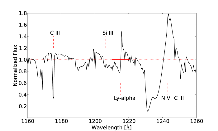
Figure 1: Theoretical spectrum of a cmfgen O star with effective temperature of 40,000 K, log$\,g$ of 3.5, and micro turbulent velocity of 10 km/s. The red dashed vertical lines mark the rest wavelength of the most prominent lines. The red horizontal dotted and solid lines mark the continuum and integration window used for the “simple integration” method (see Section 2), respectively.

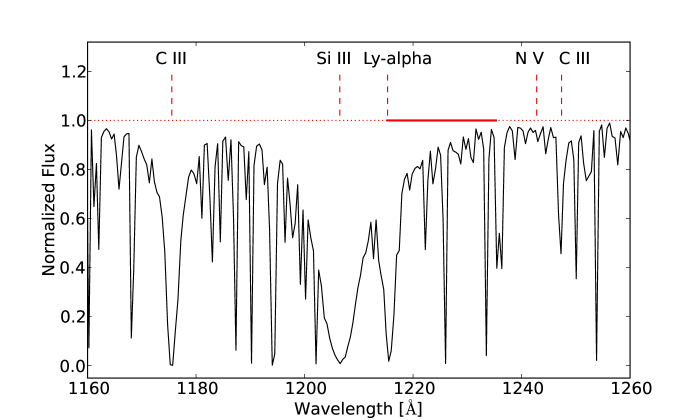
Figure 2: Theoretical spectrum of a tlusty B star with effective temperature of 18,000 K, log$\,g$ of 4.25, and micro turbulent velocity of 2 km/s. The red dashed vertical lines mark the rest wavelength of the most prominent lines. The red horizontal dotted and solid lines mark the continuum and integration window used for the “half integration” method (see Section 2), respectively.

Figures 1 and 2 show representative spectra of O and B stars, respectively. In both figures the most prominent lines are marked for reference, and the red horizontal line indicates the position of the continuum and the EW integration range for each star type. These reference lines are: C III 1175 Å, Si III 1206 Å, H I Ly$\alpha$ 1216 Å, N V 1240 Å, and C III 1247 Å. For O stars the spectra of most models show clear P Cygni profiles, indicating the combination of photospheric absorption and high density stellar winds due to radiation pressure (Leitherer et al., 1995). In the spectra of luminous O stars and even in the earliest B stars, the N V line can be quite prominent (and in some cases blend with Ly$\alpha$), though its strength decreases for later B stars (Walborn et al., 1985). In turn, the Si III line does not play a major role in the spectra of O stars but in B stars this line can easily blend with Ly$\alpha$, since the Ly$\alpha$ width increases considerably for later B type stars (Walborn et al., 1995). Since in this study we aim to determine the stellar contribution of the observed Ly$\alpha$ EW, we want to avoid most of the possible blendings with Ly$\alpha$. We therefore chose different EW integration ranges for O and B stars.

For the modeled O stars, the integration was performed over 10 Å centered on the rest frame wavelength of the Ly$\alpha$ line (strictly 1215.67 Å). The EW’s of these stars were on average in absorption and mostly close to 0 Å due to the strong P Cygni wind profiles (see Figure 1). Hence, the chosen wavelength range of 10 Å allowed us to account for the full width of Ly$\alpha$, including wings and the P Cygni profiles, if present.

For the modeled B stars, the integration was done over 40 Å centered on the rest frame wavelength of Ly$\alpha$ in order to account for the broader Ly$\alpha$ absorption. For clarity we will call this determination “simple integration” EW. Nonetheless, the Si III resonance line at 1206.5 Å is an important source of line blending for B stars (Savage & Panek, 1974). In order to correct for the contribution of this line to Ly$\alpha$ we assumed that Ly$\alpha$ was symmetric, and avoided the part of the spectrum where Si III and Ly$\alpha$ overlap. We integrated the EW from the rest wavelength of Ly$\alpha$ to Ly$\alpha$+20 Å and then multiplied this EW by 2. We call this determination “half integration” EW.

Savage & Panek (1974) found that the typical contribution of the Si III line to Ly$\alpha$ is about 4 Å. When comparing the Ly$\alpha$ EW determinations through “simple integration” EW to the “half integration” EW, we found that the difference between the first and the second EW determination is on average 3 Å but peaks between log$\,g$ of 2.0 and 2.50 to about 7 Å below an effective temperature of 21,000 K. We chose the “half integration” EW to better represent the Ly$\alpha$ EW since the Si III line is a clear systematic feature in the modeled B star spectra (see Figure 2). The resulting EW determinations for B stars are all in absorption and range from 1 to 32.5 Å.

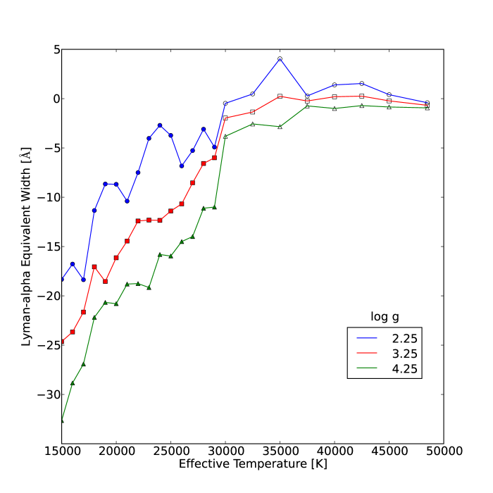
Figure 3: Plot of Ly$\alpha$ EW versus effective temperature. Three representative curves are presented. The top curve (blue circles) represents the Ly$\alpha$ EW for stars with a log$\,g$ of 2.25, the middle curve (red squares) for stars with a log$\,g$ of 3.25, and the lower curve (green triangles) for stars with log$\,g$ of 4.25. Filled symbols represent tlusty stars, while open symbols represent cmfgen stars.

For $T_{eff}$ of 15,000 to 30,000 K we used the tlusty models and for $T_{eff}$ $>30,000$ K we used the cmfgen models. We did a linear interpolation to obtain the EW’s for those values of $T_{eff}$ and log$\,g$ that were not included in the model spectra we retrieved. The final EW’s adopted in this work are presented in Table 2. Figure 3 shows the trend of our EW determinations with respect to $T_{eff}$ for different values of log$\,g$. We attribute the slight jump in this figure to the different treatments of the stellar winds used in tlusty and cmfgen codes. Nonetheless, in order to check for consistency between both codes, we studied in the differences between EW measurements in the overlapping region (i.e. $T_{eff}$ between 27,000 and 30,000 K). We found that the mode and average difference of the cmfgen and the tlusty EWs is about 7 Å, with a maximum difference of 9 Å at $T_{eff}$ of 30,000 K and log$\,g$ of 3.75.

The behavior shown in Figure 3 is consistent with what is expected from observations. For both O and B stars, the intensity and width of the ultraviolet features is closely related to the luminosity type (Walborn et al., 1995). Spectra of O stars show a P Cygni profile in some lines (late-B stars for metal lines) when the absorbing ions column density is larger than about $10^{15}$ ions per cm^-2 (Lamers & Cassinelli, 1999). This is precisely the overlapping region in our EW measurements, from 27,000 to 30,000 K. The P Cygni profiles for Ly$\alpha$ become progressively smaller as the $T_{eff}$ decreases, hence making the EW progressively differ from zero (i.e. a greater absorption as the wind emission becomes smaller). As $T_{eff}$ keeps decreasing, the Ly$\alpha$ absorption becomes wider.

In order to explore how non-solar chemical compositions affect the Ly$\alpha$ EW, we obtained spectra of tlusty of B stars with $T_{eff}$ of 30,000 K and log$\,g$ of 4.25, and with 4 different metallicities besides solar. These stars are also described in Lanz & Hubeny (2007). We determined the EW’s with the “half integration” method. The determined Ly$\alpha$ EW’s for metallicities (in units of Z/Z_☉) of 2, 1, 1/2, 1/5, and 1/10 were: -15.38, -12.87, -10.43, -9.85, and -6.30 Å, respectively. The overall shape of the spectrum changes very little with metallicity, i.e. the lines around Ly$\alpha$ become less prominent, making it easier to detect Ly$\alpha$ even considering that the EW is also getting smaller. This behavior is as expected since: (i) the EW is defined as the wavelength range over which the continuum around the line must be integrated to produce the same intensity as the observed line (Lallement et al., 2011), and (ii) the effect of metallicty on other hydrogen lines such as the Balmer lines is also rather weak if the $T_{eff}$ is higher than 7,000 K (González-Delgado & Leitherer, 1999).

3 Comparison with Observations of O and B stars

In order to gain confidence into our set of Ly$\alpha$ EW’s, we surveyed the literature for available observations of stellar Ly$\alpha$. There is a rich body of data dating back to the early observations by OAO-2 (Savage & Jenkins, 1972), OAO-3 (Bohlin et al., 1978), and IUE (Diplas & Savage, 1994a, b). We compared our theoretical Ly$\alpha$ EW determinations with those from observations of O and B stars presented in Savage & Code (1970) and Savage & Panek (1974). The observations presented in Savage & Code and Savage & Panek were taken with OAO-2, whose spectrograph had a resolution of 15 Å. The relatively low resolution implies that there could be contamination with Si III on the short-wavelength side of Ly$\alpha$ and possibly with N V on the long-wavelength side, depending on the extent of the wings of Ly$\alpha$.

We adopted the EW’s as published by Savage & Code (1970) and Savage & Panek (1974), with the sign convention used through out this work. Contamination of stellar Ly$\alpha$ by the interstellar H I absorption is a serious concern, in particular for O stars whose larger average distances (when compared to B stars) lead to interstellar neutral hydrogen column densities $N_{H}$ in excess of $10^{20}$ cm^-2. As a result, the measured Ly$\alpha$ EW’s in essentially all O stars are not stellar but interstellar. Since the derived lower limits of the stellar contribution to the total Ly$\alpha$ would provide little insight into the validity of our models, we did not consider stars with $T_{eff}$$>35,000$ K for our comparison. This cut-off corresponds to spectral type O9. In Table 3 we present the selected stars together with the pertinent parameters. Columns 1 and 2 list the designations. The spectral types are in column 3. $T_{eff}$ (column 4) was assigned using the calibration of Conti et al. (2008). Observed EW values are in column 5.

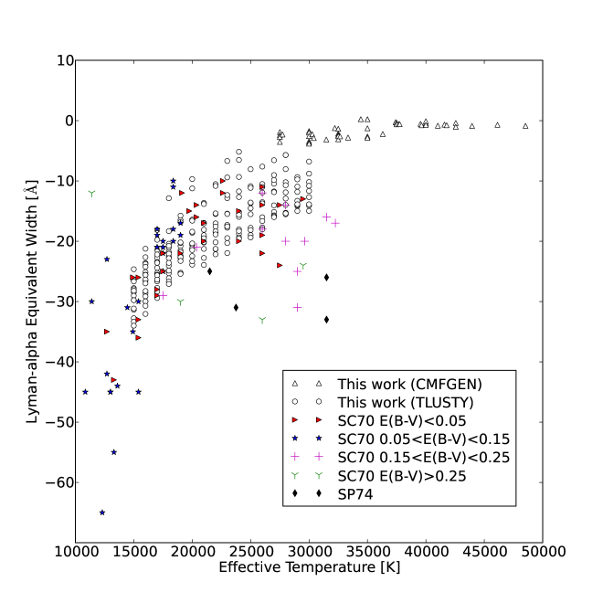
Figure 4: Comparison between our Ly$\alpha$ EW determinations and those from observations, as a function of effective temperature. Symbols represent the following: open up triangles are EW determinations of this work, from cmfgen models, open circles are EW determinations from tlusty models, red rotated triangles, magenta crosses, black diamonds, and green three-pointed stars are EW obtained from observations from Savage & Code (1970), SC70, for different values of $E(B-V)$, and blue stars are EW obtained from observations from Savage & Panek (1974), SP74. SC70 measurements are blended with the interstellar Ly$\alpha$ line and with neighboring lines, and SP74 are corrected for both ISM and blending with the Si III.

In Figure 4 we show the comparison between the observed and theoretical EW values as a function of stellar effective temperature. The models display a near-monotonic trend with $T_{eff}$, asymptotically reaching about zero Å at $T_{eff}$ $>35,000$ K. At a given $T_{eff}$, a larger log$\,g$ results in stronger Ly$\alpha$ absorption. The observed values track the models very well at the lowest temperatures but tend to be more negative (stronger absorption) at higher temperatures (corresponding to early B stars). We interpret this as not due to a model failure but rather being caused by residual interstellar contamination. In support of this suggestion we indicated the measured $E(B-V)$ values for each observation, taken from Savage & Code (1970) and Savage & Panek (1974). There is a clear trend of the largest discrepancies between models and data occurring for the highest $E(B-V)$ values. Since there is a well-established relation between $E(B-V)$ and interstellar $E(B-V)$ (Diplas & Savage, 1994a), we conclude that the majority of the observational points below the models are in fact just lower limits to the stellar contribution.

The outcome of the comparison between the modeled and observed EW’s is quite reassuring. While there are few observational constraints on the Ly$\alpha$ EW in O stars, the intrinsic Ly$\alpha$ in the hottest stars is expected to be weak because of the counteracting effects of photospheric absorption and wind emission. Therefore these stars would make only minor contribution to the total stellar absorption in a representative population. B stars, on the other hand, when present in a population can contribute substantially, and their modeled Ly$\alpha$ is in very good agreement with the data.

4 Population Synthesis Models

The Ly$\alpha$ EW’s listed in Table 2 were implemented in the synthesis code Starburst99 (Leitherer et al., 1999; Leitherer & Chen, 2009). We performed a 2-dimensional interpolation in $T_{eff}$ and log$\,g$ to obtain the EW values for each point in the Hertzsprung-Russell diagram as prescribed by the stellar evolutionary tracks. The input table is essentially complete at the highest temperatures, and no significant extrapolations were required. For $T_{eff}$ between 15,000 K and 10,000 K (late B stars) we used eq. (1) of Valls-Gabaud (1993) to approximate the Ly$\alpha$ EW. No attempts was made to account for EW at even lower $T_{eff}$, and we simply assumed a featureless continuum for $T_{eff}$ $<10,000$ K. This means our models are no longer valid when A stars begin to contribute to the UV continuum. We do not distinguish between O- and Wolf-Rayet stars when assigning Ly$\alpha$ EW’s to stars in the Hertzsprung-Russell diagram. The underlying assumption is that Ly$\alpha$ (or the He II line at approximately the same wavelength) in Wolf-Rayet stars behaves in a similar fashion as in hot O stars.

The nebular Ly$\alpha$ was calculated assuming standard Case B recombination for an electron temperature of $10^{4}$ K. For reference, the Ly$\alpha$/H$\alpha$ ratio is 8.7 under these assumptions (Case A would be 11.4).

We created a standard set of synthetic Ly$\alpha$ EW for evolving stellar populations using the Geneva evolution models with high mass loss at solar chemical composition (Meynet et al., 1994). As a consistency check, we compared our predictions with those published in the literature. A standard Salpeter initial mass function (IMF) has been adopted for these comparisons. Charlot & Fall (1993) and Valls-Gabaud (1993) were the first to draw attention to the importance of underlying stellar Ly$\alpha$ for the interpretation of nebular Ly$\alpha$ in star-forming galaxies. They both used the original Bruzual & Charlot (1993) evolutionary synthesis models with a correction of stellar Ly$\alpha$ to predict the net nebular + stellar Ly$\alpha$. The stars evolve along the tracks computed by Maeder & Meynet (1989) in these models. In Table 4 we compare their and our predictions for selected ages and for the two limiting cases of an instantaneous burst and continuous star formation. Also included in Table 4 are the predictions of Schaerer & Verhamme (2008) who used a modified version of the Schaerer (2003) evolutionary synthesis models for predictions of nebular + stellar Ly$\alpha$. The different sets of models are in reasonable agreement. The differences reflect the use of different evolutionary tracks and different model atmospheres. Note in particular that the larger EW at age $5\times 10^{6}$ yr in the Charlot & Fall and Valls-Gabaud models is the result of different life times in the stellar evolution models. At this age, the nebular Ly$\alpha$ displays a sharp drop with age, and a slight shift in age causes a vastly different ionizing photon output.

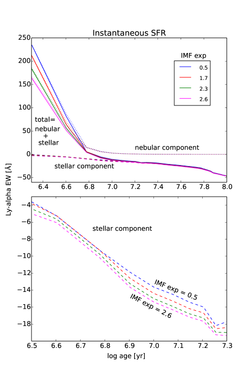
Figure 5: Ly$\alpha$ EW’s versus age for an instantaneous burst. This figure shows a series of Starburst99 runs for different IMF exponents, labeled by color from 0.5 (blue) through 2.6(magenta). Salpeter is represented by the green curve. Dashed lines represent the stellar component of Ly$\alpha$ EW, dotted lines represent the nebular component, and solid lines the total component. The sign convention used for this work is positive for emission and negative for absorption. The upper panel shows the overall behavior of Ly$\alpha$ up to 100 million years. The bottom panel shows a zoom-in of the stellar component from about 3 to 20 million years.

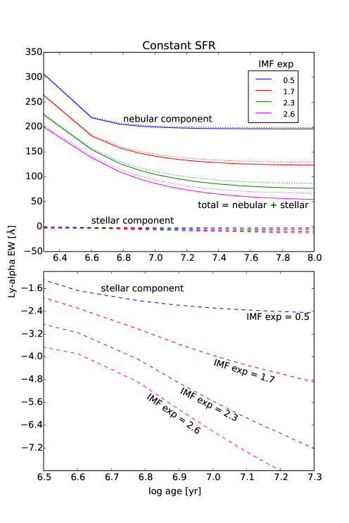
Figure 6: Same as Figure 5 but for constant star formation rate.

We performed a parameter study in order to analyze the impact of different IMF s, different ages, and different star-formation histories in the Ly$\alpha$ EW s. The two bracketing cases of an instantaneous burst and constant star formation were considered. Starburst99 assumes a power-law IMF of the classical form $\phi(m)\propto m^{-\alpha}$. In this notation, the classical Salpeter IMF has an exponent of $\alpha=2.35$. In Figures 5 and 6 we show the resulting Ly$\alpha$ EW s for different IMF slopes in the case of an instantaneous burst and continuous star formation, respectively.

We first address the relative importance of the underlying stellar Ly$\alpha$ at different ages in each of the two cases. The burst models (Fig. 5) fall into two regimes: at young ages (t $\lesssim$ 6 Myr), the nebular part always dominates since copious O stars photons are available and O stars have intrinsically weak Ly$\alpha$. At older ages (t $\gtrsim$10 Myr), the starburst is B-star dominated with few ionizing photons but at the same time intrinsically strong stellar Ly$\alpha$. In the case of continuous star formation (Figure 6), the nebular component always dominates, and the underlying stellar Ly$\alpha$ is always negligible. As a reminder, this assumes pure Case A recombination for the nebular Ly$\alpha$  with a 100% photon escape.

Different IMF exponents, ranging from an extreme, flat IMF of $\alpha=0.5$ to another extreme, steep value of $\alpha=2.6$, only have a minor influence in the stellar Ly$\alpha$ EW s. The equivalent width varies by about 2 Å for the considered IMF exponents between 0.5 and 2.6 for an instantaneous burst. This is expected for a single population where the stellar flux at a particular wavelength comes from stars over a very narrow mass range. In the continuous case, the IMF sensitivity of the stellar Ly$\alpha$ is somewhat more pronounced but still quite minor.

Next, we turn to the IMF dependence of the nebular component of Ly$\alpha$. The IMF has a much more pronounced effect in this case, which can easily be understood from the fact the EW(Ly$\alpha$) is determined by the ratio of early- to late-O stars, which contribute the ionizing photons and the continuum. Varying the IMF slope will change the relative contributions of these species. Therefore the IMF behavior in Figs. 5 and 6 is not surprising and mirrors that of, e.g., the H$\alpha$ or H$\beta$ equivalent width, which has been extensively discussed in the literature (Leitherer et al., 1999).

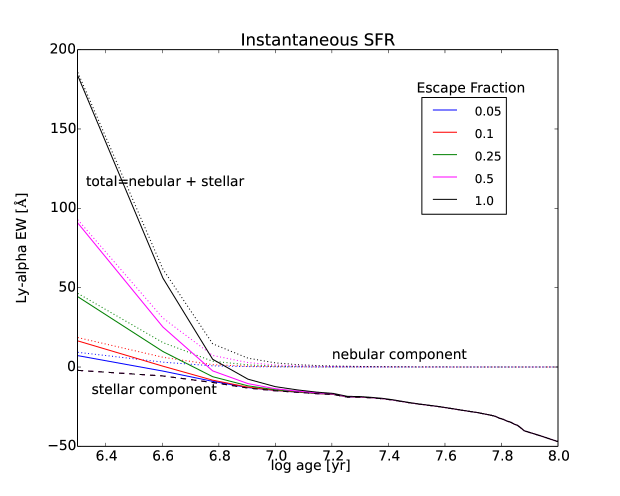
Figure 7: Ly$\alpha$ EW’s versus age for an instantaneous burst for different Ly$\alpha$ escape fractions. This figure shows a series of Starburst99 runs for an IMF exponent of 2.3. Dashed lines represent the stellar component of Ly$\alpha$ EW, dotted lines represent the nebular component, and solid lines the total component. The sign convention used for this work is positive for emission and negative for absorption.

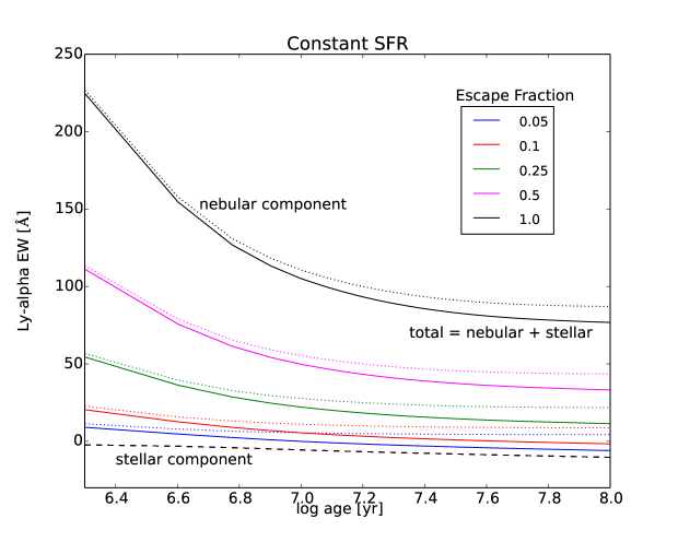
Figure 8: Same as Figure 7 but for constant star formation rate.

The previous discussion is based on the assumption of a 100% escape probability of the nebular Ly$\alpha$ photons. Observations suggest a much lower escape fraction. For instance the Ly$\alpha$ EW s observed in Lyman-break galaxies at redshift $\sim 3$ are of order 10 Å (Shapley et al., 2003). Comparison with our continuous models uncorrected for stellar absorption, implies an escape of Ly$\alpha$ photons of $\sim 10$%. In order to provide a more realistic model grid for comparison with data, we generated models with a Salpeter IMF and nebular Ly$\alpha$ escape fractions of 5, 10, 25, 50 and 100%. These models are plotted in Figures 7 and 8 for instantaneous bursts and continuous star formation, respectively. Because of the reduced nebular emission for escape fractions less than 100%, the underlying stellar absorption drastically increases in its contribution to the net EW. For instance, if the escape fraction is 10% the stellar absorption and nebular emission EW’s become comparable for continuous star formation at ages of 10 to 20 Myr.

5 Conclusions

We present a grid of theoretical stellar Ly$\alpha$ equivalent widths for evolving stellar populations. While these models have value in their own right, our main motivation for presenting the grid is the need to correct nebular Ly$\alpha$ emission in star-forming galaxies for underlying stellar absorption. This study builds on the pioneering work of Valls-Gabaud (1993) and Charlot & Fall (1993) who had to rely on earlier, less complete model atmospheres, and it extends the exploratory work of Schaerer & Verhamme (2008), who used the latest model atmospheres for a restricted parameter range.

We compiled a new library of non-LTE Ly$\alpha$ EW s based on fully line-blanketed models. The library includes O and B stars with effective temperatures ranging from 15,000 K to 48,500 K, and log$\,g$ from 1.75 to 4.5. The measured Ly$\alpha$ EW’s range from 5.9 to -32.5 Å. In particular, we obtained: Ly$\alpha$ EW between 0.9 and -32.5 Å for effective temperatures of 15,000 K to 29,000 K, and values mostly close to 0 Å for higher effective temperatures due to the canceling effects of the emission and absorption of the P Cygni profiles of these stars. Metallicity has very little effect on the Ly$\alpha$ EW’s.

We implemented the library in Starburst99 and studied the behavior of the Ly$\alpha$ EW for a range of stellar population properties. We performed a parameter study of instantaneous and continuous star formation at solar metallicity, using the high-mass loss Geneva evolution models (Meynet et al., 1994). We found: (i) The IMF has only minor influence on the stellar EW when varied within astrophysically plausible limits for both an instantaneous and a constant SFR. (ii) The IMF has also a minor influence on the nebular component of the Ly$\alpha$ EW for an instantaneous SFR, however, for a continuous SFR, the difference between the two extreme IMF exponents (0.5 and 2.6) in the nebular component of the Ly$\alpha$ EW is about 100 Å at 3 Myr and about 180 Å at 15 Myr. (iii) When O stars dominate the spectrum (as indicated by the presence of nebular emission lines), stellar Ly$\alpha$ absorption is always small compared to gaseous Ly$\alpha$ (if nebular Ly$\alpha$ has an escape fraction close to 100%). (iv) Depending on the escape fraction of nebular Ly$\alpha$ photons, the stellar contribution to the total ranges from negligible to dominant. If the nebular escape fraction is 10%, the stellar absorption and nebular emission equivalent widths become comparable for continuous star formation at ages of 10 to 20 Myr.

In stark contrast to the often used a stellar absorption correction of 50 to 240 Å, our models predict: (i) stellar Ly$\alpha$ EW values of 9 to 18 Å in absorption for an instantaneous burst between the ages of 5 to 15 Myr, and (ii) values of 2 to 8 Å also in absorption for constant star formation in the same age range. Our models provide a realistic description of the stellar Ly$\alpha$ and should be appropriate to correct the nebular emission for underlying stellar absorption in star-forming galaxies.

AKNOWLEDGEMENTS. We are grateful to an anonymous referee for a careful reading of the manuscript and many useful suggestions. We are also grateful to John Hillier for kindly providing us with plane-parallel cmfgen models to check consistency between the results of cmfgen and tlusty modeled atmospheres. Support for this work has been provided by NASA through grant number N-1317 from the Space Telescope Science Institute, which is operated by AURA, Inc., under NASA contract NAS5-26555.

Table 1: Parameters of the models used for the new library.

$T_{eff}$ [K]	log$\,g$	Code
15,000	1.75, 2.00, 2.25, 2.50, 2.75, 3.00, 3.25, 3.50, 3.75, 4.00, 4.25, 4.50	tlusty
16,000	2.00, 2.25, 2.50, 2.75, 3.00, 3.25, 3.50, 3.75, 4.00, 4.25, 4.50	tlusty
17,000	2.00, 2.25, 2.50, 2.75, 3.00, 3.25, 3.50, 3.75, 4.00, 4.25, 4.50	tlusty
18,000	2.00, 2.25, 2.50, 3.00, 3.25, 3.50, 3.75, 4.00, 4.25, 4.50	tlusty
19,000	2.25, 2.50, 2.75, 3.00, 3.25, 3.50, 3.75, 4.00, 4.25, 4.50	tlusty
20,000	2.25, 2.50, 2.75, 3.00, 3.25, 3.50, 3.75, 4.00, 4.25, 4.50	tlusty
21,000	2.50, 2.75, 3.00, 3.25, 3.50, 3.75, 4.00, 4.25, 4.50	tlusty
22,000	2.50, 2.75, 3.00, 3.25, 3.50, 3.75, 4.00, 4.25, 4.50	tlusty
23,000	2.50, 2.75, 3.00, 3.25, 3.50, 3.75, 4.00, 4.25, 4.50	tlusty
24,000	2.50, 2.75, 3.00, 3.25, 3.50, 3.75, 4.00, 4.25, 4.50	tlusty
25,000	2.50, 2.75, 3.00, 3.25, 3.50, 3.75, 4.00, 4.25, 4.50	tlusty
26,000	2.75, 3.00, 3.25, 3.50, 3.75, 4.00, 4.25, 4.50	tlusty
27,000	2.75, 3.00, 3.25, 3.50, 3.75, 4.00, 4.25, 4.50	tlusty
27,500	3.00, 3.75	cmfgen
27,730	3.35	cmfgen
28,000	2.75, 3.00, 3.25, 3.50, 3.75, 4.00, 4.25, 4.50	tlusty
29,000	3.00, 3.25, 3.50, 3.75, 4.00, 4.25, 4.50	tlusty
30,000	3.00, 3.25, 3.50, 3.75, 4.00, 4.25, 4.50	tlusty
30,000	3.00, 3.13, 3.50, 4.00, 4.10, 4.20	cmfgen
30,270	3.29	cmfgen
30,410	3.73	cmfgen
31,480	4.06	cmfgen
32,210	3.26	cmfgen
32,500	3.25, 3.50, 3.60, 4.10, 4.25	cmfgen
32,660	3.71	cmfgen
33,340	4.01	cmfgen
34,435	3.52	cmfgen
35,000	3.25, 3.50, 4.10, 4.25	cmfgen
36,310	4.02	cmfgen
37,411	3.38	cmfgen
37,500	3.50, 3.90	cmfgen
37,670	3.77	cmfgen
37,760	3.76	cmfgen
39,540	3.68	cmfgen
39,628	3.93	cmfgen
39,994	3.63	cmfgen
40,000	3.50, 3.90	cmfgen
41,020	4.04	cmfgen
41,591	3.80	cmfgen
41,178	4.02	cmfgen
42,560	3.71	cmfgen
42,560	4.16	cmfgen
43,954	3.98	cmfgen
46,130	4.05	cmfgen
48,530	4.01	cmfgen

Table 2: Ly$\alpha$ Equivalent Widths as a function of Effective Temperature and log$\,g$.

$T_{eff}$[K]		Ly$\alpha$ EW [Å] for log$\,g$ of:
		1.75	2.00	2.25	2.50	2.75	3.00	3.25	3.50	3.75	4.00	4.25	4.50
15,000		-15.3	-20.6	-18.3	-22.6	-25.5	-25.6	-24.6	-27.9	-29.3	-29.3	-32.6	-32.5
16,000		-12.2	-13.8	-16.8	-17.8	-19.8	-20.8	-23.7	-24.2	-25.0	-27.5	28.8	-29.7
17,000		-9.6	-11.1	-18.4	-16.0	-16.6	-19.7	-21.7	-21.7	-23.8	-24.6	-26.9	-25.9
18,000		-3.8	-5.7	-11.4	-13.6	-15.5	-15.4	-17.1	-19.4	-20.3	-24.4	-22.2	-24.3
19,000		-5.2	-7.0	-8.7	-9.4	-15.7	-14.3	-18.5	-18.6	-20.6	-19.8	-20.7	-24.1
20,000		-5.8	-7.2	-8.7	-11.5	-13.6	-13.6	-16.1	-15.5	-18.01	-17.9	-20.8	-21.7
21,000		-8.1	-9.2	-10.4	-11.6	-10.8	-12.5	-14.5	-14.4	-16.9	-17.9	-18.8	-20.9
22,000		-5.0	-6.3	-7.5	-8.7	-10.6	-12.2	-12.4	-14.9	-15.2	-16.9	-18.8	-18.6
23,000		-1.3	-2.7	-4.0	-5.4	-10.9	-11.0	-12.3	-12.2	-14.8	-14.3	-19.2	-16.2
24,000		0.9	-0.9	-2.7	-4.5	-9.0	-10.0	-12.4	-13.5	-15.7	-17.0	-15.8	-18.8
25,000		-0.7	-2.2	-3.7	-5.3	-6.8	-11.2	-11.4	-11.9	-12.7	-16.3	-16.0	-17.5
26,000		-4.8	-5.8	-6.8	-7.8	-8.8	-9.6	-10.6	-10.7	-14.1	-12.9	-14.5	15.9
27,000		-3.5	-4.4	-5.3	-6.2	-7.0	-10.4	-8.5	-10.0	-12.2	-11.8	-14.0	-13.2
28,000		-1.0	-2.0	-3.1	-4.2	-5.2	-7.5	-6.6	-8.1	-11.2	-12.8	-11.1	-12.7
29,000		-3.5	-4.2	-4.9	-5.6	-6.3	-7.0	-6.0	-8.0	-11.0	-12.0	-11.0	-11.2
30,000		0.4	-0.1	-0.5	-0.9	-1.3	-1.7	-2.0	-2.6	-3.0	-3.4	-3.8	-4.3
32,500		1.5	1.0	0.5	-0.0	-0.5	-1.1	-1.4	-2.1	-2.4	-3.1	-2.6	-4.1
35,000		5.9	5.0	4.0	3.1	2.1	1.2	0.2	-1.3	-1.7	-2.6	-2.8	-4.5
37,500		0.5	0.4	0.3	0.1	0.0	-0.1	-0.2	-0.4	-0.5	-0.6	-0.7	-0.9
40,000		2.0	1.7	1.4	1.1	0.8	0.5	0.2	-0.1	-0.4	-0.7	-1.0	-1.3
42,500		2.2	1.8	1.5	1.2	0.9	0.5	0.3	-0.1	-0.4	-0.7	-1.0	-1.4
45,000		0.7	0.6	0.4	0.2	0.1	-0.1	-0.2	-0.4	-0.5	-0.7	-0.9	-1.0
48,500		-0.3	-0.4	-0.4	-0.5	-0.6	-0.6	-0.7	-0.7	-0.8	-0.9	-0.9	-1.0

Table 3: Ly$\alpha$ Equivalent Widths Measurements from Observations as a function of Effective Temperature.

Star	Name	Spectral Type	Ly$\alpha$ EW[Å]	$T_{eff}$ [K]
[HD number]
Taken from Savage & Code (1970)
11415	$\epsilon$ Cas	B3 IVp	-28	17,500
24398	$\zeta$ Per	B1 Ib	-25	21,500
24760	$\epsilon$ Per	B0.5 V	-14	28,000
29763	$\tau$ Tau	B3 V	-29	17,500
32630	$\eta$ Au	B3 V	-25	17,500
34816	$\lambda$ Lep	B0.5 IV	-14	27,500
35411	$\eta$ Ori	B0.5 V	-20	28,000
35439	25 Ori	B1 Vpe	-19	26,000
35468	$\gamma$ Ori	B2 III	-15	19,750
35497	$\beta$ Tau	B7 III	-35	12,700
36485-86	$\delta$ Ori	O9.5 II	-20	29,625
36512	$\nu$ Ori	B0 V	-13	29,500
36822	$\phi^{\prime}$ Ori	B0 IV	-31	29,000
37022	41 Ori	O7 V		37,000
-41	$\theta$ Ori	O9.5 Vp	-33	31,500
37043	$\iota$ Ori	O9 III	-17	32,250
37128	$\epsilon$ Ori	B0 Ia	-24	27,500
37202	$\zeta$ Tau	B2 IVp	-21	20,375
37468	$\sigma$ Ori	O9.5 V	-16	31,500
37742-43	$\zeta$ Ori	O9.5 Ib	-25	29,000
38771	$\kappa$ Ori	B0.5 Ia	-22	26,000
44743	$\beta$ CMa	B1 II	-10	22,625
52089	$\epsilon$ CMa	B2 II	-12	19,125
87901	$\alpha$ Leo	B7 V	-43	13,300
116658	$\alpha$ Vir	B1 V	-11	26,000
120315	$\eta$ Uma	B3 V	-22	17,500
122451	$\beta$ Cen	B1 II	-12	22,625
127381	$\sigma$ Lup	B2 V	-20	21,000
127972	$\eta$ Cen	B1.5 Vne	-15	24,000
128345	$\rho$ Lup	B5 V	-36	15,400
129056	$\alpha$ Lup	B1 V	-14	26,000
132200	$\kappa$ Cen	B2 V	-17	21,000
133242-43	$\pi$ Lup	B5 IV	-26	14,925
133955	$\lambda$ Lup	B3 V	-22	17,500
136298	$\delta$ Lup	B2 IV	-14	20,375
136664	$\phi^{2}$ Lup	B5 V	-26	15,400
139365	$\tau$ Lib	B2.5 V	-22	19,000
141637	1 Sco	B2.5 Vn	-30	19,000
142983	48 Lib	B8 Ia/Iab	-12	11,400
143018	$\pi$ Sco	B1 V	-18	26,000
143275	$\delta$ Sco	B0 V	-24	29,500
144470	$\omega^{1}$ Sco	B1 V	-33	26,000
147165	$\sigma$ Sco	B1 III	-31	23,750
149757	$\zeta$ Oph	O9.5 V	-26	31,500
151890	$\mu^{\prime}$ Sco	B1.5 V	-20	24,000
158926	$\lambda^{\prime}$ Sco	B1 V	-12	26,000
160578	$\kappa$ Sco	B2 IV	-16	20,375
189103	$\Theta^{\prime}$ Sgr	B3 IV	-29	17,000
209952	$\alpha$ Gru	B5 V	-33	15,400
Taken from Savage & Panek (1974)
358	$\alpha$ And	B9 II	-45	10,850
10144	$\alpha$ Eri	B3 Vp	-21	17,500
11415	$\epsilon$ Cas	B3 Vp	-25	17,500
19356	$\beta$ Per	B8 V	-65	12,300
22928	$\delta$ Per	B5 III	-31	14,450
32630	$\eta$ Aur	B3 V	-22	17,500
34085	$\beta$ Ori	B8 Ia	$>$-30	11,400
35497	$\beta$ Tau	B7 III	-42	12,700
37795	$\alpha$ Col	B7 IV	-45	13,000
42560	$\xi$ Ori	B3 IV	-21	17,000
44402	$\zeta$ CMa	B2.5 IV	-20	18,375
6575	$\chi$ Car	B3 IVp	-19	17,000
87901	$\alpha$ Leo	B7 V	-55	13,300
120315	$\eta$ UMa	B3 V	-25	17,500
121263	$\zeta$ Cen	B2.5 IV	-10	18,375
125238	$\iota$ Lup	B2.5 IV	-18	18,375
125823	$\alpha$ Cen	B7 IIIp	-23	12,700
128345	$\rho$ Lup	B5 V	-45	15,400
129116		B3 V	-20	17,500
133242	$\pi$ Lup	B5 V	-30	15,400
-43		B5 IV		14,975
133955	$\lambda$ Lup	B3 V	-21	17,500
139365	$\tau$ Lib	B2.5 V	-19	19,000
143118	$\eta$ Lup	B2.5 IV	-11	18,375
147394	$\tau$ Her	B5 IV	-35	14,925
155763	$\zeta$ Dra	B6 III	-44	13,600
160762	$\iota$ Her	B3 IV	-21	17,000
175191	$\sigma$ Sgr	B3 IV	-18	17,000
193924	$\alpha$ Pav	B2.5 V	-17	19,000
209952	$\alpha$ Gru	B7 IV	-45	13,000

Table 4: Comparison of Ly$\alpha$ Equivalent Widths. These values where determined for a Salpeter IMF, a stellar population with ages 5$\times 10^{6}$ and 15$\times 10^{6}$ years, and solar metallicity.

Authors		Stellar component EW [Å]			Nebular component EW [Å]			Total EW [Å] = stellar + nebular
		5$\times 10^{6}$ years	15$\times 10^{6}$ years		5$\times 10^{6}$ years	15$\times 10^{6}$ years		5$\times 10^{6}$ years	15$\times 10^{6}$ years
Instantaneous SFR
This work		-8	-17		40	1		32	-16
Charlot & Fall (1993)		$\cdots$	$\cdots$		$\cdots$	$\cdots$		210	53
Valls-Gabaud (1993)		-5	-15		205	5		200	-10
Schaerer & Verhamme (2008)		-4	-20		47	3		43	-17
Constant SFR
This work		-4	-7		145	100		141	93
Charlot & Fall (1993)		$\cdots$	$\cdots$		$\cdots$	$\cdots$		217	110
Valls-Gabaud (1993)		-3	-5		253	195		250	190
Schaerer & Verhamme (2008)		-1	-4		131	80		130	76

References

- Bohlin et al. (1978) Bohlin, R. C., Savage, B. D., & Drake, J. F. 1978, ApJ, 224, 132
- Bromm & Yoshida (2011) Bromm, V. & Yoshida, N. 2011, A&A, 49, 373
- Bruzual & Charlot (1993) Bruzual, G. & Charlot, S. 1993, ApJ, 405, 538
- Charlot & Fall (1993) Charlot, S. & Fall, M. 1993, ApJ, 415, 580
- Conti et al. (2008) Conti, P. S., Crowther, P. A., & Leitherer, C. 2008, “From Luminous Hot Stars to Starburst Galaxies”, Cambridge University Press, Cambridge, UK
- Dijkstra & Wyithe (2010) Dijkastra, M. & Wyithe, S. B. 2010, MNRAS, 408, 352
- Dijkstra & Wyithe (2012) Dijkastra, M. & Wyithe, S. B. 2012, MNRAS, 419, 3181
- Diplas & Savage (1994a) Diplas, A. & Savage, B. 1994a, ApJ, 427, 274
- Diplas & Savage (1994b) Diplas, A. & Savage, B. 1994b, ApJS, 93, 211
- Fujita et al. (2003) Fujita, S. S., Ajiki, M., Shioya, Y., et al. 2003, AJ, 125, 13
- Giavalisco, Koratkar & Calzetti (1996) Giavalisco, M., Koratkar, A., & Calzetti, D. 1996, ApJ, 446, 831
- González-Delgado & Leitherer (1999) González-Delgado, R. M. & Leitherer, C. 1999, ApJ, 125, 479
- Haiman & Spaans (1999) Haiman, Z. & Spaans, M. 1999, AIPC, 470, 63
- Hansen & Oh (2006) Hansen, M. & Oh, S. P. 2006, MNRAS, 367, 979
- Hartmann et al. (1988) Hartmann, L. W., Huchra, J. P., Geller, M. J., O’Brien, P., & Wilson, R. 1988, ApJ, 326, 101
- Heap, Lanz, & Hubeny (2006) Heap, S. R., Lanz, T., & Hubeny, I. 2006, ApJ, 638, 409
- Hillier (1987) Hillier, D. J. 1987, ApJS, 63, 947
- Hillier (2011) Hillier, D. J. 2011. Hot Stars with Winds: The cmfgen Code. Proceedings of the International Astronomical Union, 7, pp 229-234. doi:10.1017/S1743921311027426.
- Hillier & Lanz (2001) Hillier, D. J. & Lanz, T. 2001, ASPC, 247, 343
- Hillier & Miller (1998) Hillier, D. J. & Miller, D. L. 1998, ApJ, 496, 407
- Hubeny & Lanz (1995) Hubeny, I., & Lanz, T., 1995, AJ, 439, 875
- Kennicutt & Evans (2012) Kennicutt, R. C. & Evans, N. J. 2012, ARA&A, 50, 531
- Klein & Castor (1978) Klein, R. I. & Castor, J. I. 1978, ApJ, 220, 902
- Kunth et al. (2003) Kunth, D., Leitherer, C., Mas-Hesse, J. M., ’́Ostlin, G., & Petrosian, A. 2003, ApJ, 597, 263
- Lallement et al. (2011) Lallement, R., Quémarais, E., Bertaux, J. L., et al. 2011. Science Magazzine, Vol. 334, www.sciencemag.org
- Lamers & Cassinelli (1999) Lamers, H. J. G. L. M., & Cassinelli, J. P. 1999, Introduction to Stellar Winds, ed. H. J. G. L. M. Lamers & J. P. Cassinelli
- Lanz & Hubeny (2003) Lanz, T. & Hubeny, I. 2003, ApJS, 147, 225
- Lanz & Hubeny (2007) Lanz, T. & Hubeny, I. 2007, ApJS, 169, 83
- Laursen, Duval & Östlin (2013) Laursen, P., Duval, F., & Östlin, G. 2013, ApJ, 766, 124
- Leitherer & Chen (2009) Leitherer, C. & Chen, J. 2009, New A. 4, 356
- Leitherer et al. (2010) Leitherer, C., Ortiz, P., Bresolin, F., et al. 2010, ApJSS, 189, 309
- Leitherer et al. (1995) Leitherer, C., Robert, C., & Heckman T. M. 1995, 99, 173
- Leitherer et al. (1999) Leitherer, C., Schaerer, D., Goldader, J., et al. 1999, ApJ, 123, 3
- Maeder & Meynet (1989) Maeder, A., & Meynet, G. 1989, A&A, 210, 155
- Malhotra & Rhoads (2002) Malhotra, S. & Rhoads, J. 2002, ApJ, 565, L71
- Malhotra & Rhoads (2004) Malhotra, S. & Rhoads, J. 2004, ApJ, 617, L5
- Mas-Hesse et al. (2003) Mas-Hesse, J. M., Kunth, D., Tenorio-Tagle, G., Leitherer, C., Terlevich, R. J., & Terlevich, E. 2003, ApJ, 598, 858
- Massey et al. (2013) Massey, P., Neugent, K. F., Hillier, J. D., & Puls, J. 2013, to be published in AJ, arXiv: 1303.5469v1
- Meier & Terlevich (1981) Meier, D. L. & Terlevich, R. 1981, ApJ, 247L, 109
- Meynet et al. (1994) Meynet, G., Maeder, A., Schaeller, G., et al. 1994, A&A, 103, 97
- Neufeld (1990) Neufeld, D. 1990, ApJ, 350, 216
- Palacios et al. (2010) Palacios, A., Gebran, M., Josselin, E., et al. 2010, A&A, 516, 13
- Partridge & Peebles (1967) Partridge, R. B. & Peebles, P. J. E. 1967, ApJ, 147, 868
- Puls, Vink, & Najarro (2008) Puls, J., Vink, J. S., & Najarro, F. 2008, A&A, 16, 209
- Sandberg et al. (2013) Sandberg, A., Östlin, G., Hayes, M., et al. 2013, A&A, 552, id.A95
- Savage & Code (1970) Savage, B. D. & Code, A. D. 1970, in Ultraviolet Stellar Spectra and Related Ground-based Observations (IAU Symposium No. 36) ed. Houziaux, L. and Butler, H. E. (Dordrecht: D. Reidel Publishing Co.), p. 302
- Savage & Jenkins (1972) Savage, B. D. & Jenkins, E. B. 1972, ApJ, 172, 491
- Savage & Panek (1974) Savage, B. D. & Panek, R. J. 1974, ApJ, 191, 659
- Scarlata et al. (2009) Scarlata, C, Colbert, J., Teplitz, H. I., et al. 2009, ApJ, 704, L98
- Shapley et al. (2003) Shapley, A. E., Steidel, C. C., Pettini, M., & Adelberger, K. L. 2003, ApJ, 588, 65
- Schaerer (2003) Schaerer, D. 2003, A&A, 397, 527