The Gaussian Two-way Diamond Channel
Abstract
††footnotetext: This work was done at the Department of Electrical Engineering, IIT Madras, Chennai. India. Prathyusha V is now with Cisco Systems, Bangalore, India. Srikrishna Bhashyam and Andrew Thangaraj are with the Department of Electrical Engineering, IIT Madras, Chennai, India.We consider two-way relaying in a Gaussian diamond channel, where two terminal nodes wish to exchange information using two relays. A simple baseline protocol is obtained by time-sharing between two one-way protocols. To improve upon the baseline performance, we propose two compute-and-forward (CF) protocols – Compute-and-forward-Compound multiple access channel (CF-CMAC) and Compute-and-forward-Broadcast (CF-BC). These protocols mix the two flows through the two relays and achieve rates better than the simple time-sharing protocol. We derive an outer bound to the capacity region that is satisfied by any relaying protocol, and observe that the proposed protocols provide rates close to the outer bound in certain channel conditions. Both the CF-CMAC and CF-BC protocols use nested lattice codes in the compute phases. In the CF-CMAC protocol, both relays simultaneously forward to the destinations over a Compound Multiple Access Channel (CMAC). In the simpler CF-BC protocol’s forward phase, one relay is selected at a time for Broadcast Channel (BC) transmission depending on the rate-pair to be achieved. We also consider the diamond channel with direct source-destination link and the diamond channel with interfering relays. Outer bounds and achievable rate regions are compared for these two channels as well. Mixing of flows using the CF-CMAC protocol is shown to be good for symmetric two-way rates.
I Introduction
The half-duplex Gaussian diamond channel where a source communicates with a destination through two non-interfering relays is a problem of interest in information theory [1]. In [2], multihopping decode-and-forward (MDF) protocols were proposed to achieve rates within a constant gap of a capacity outer bound.
Two-way relaying where two nodes without a direct link communicate with each other through a single relay has been studied in [3, 4, 5, 6, 7, 8]. In [3, 4, 5], the achievable rate regions of various two-way relaying protocols are compared. In [6, 7, 8], coding strategies based on nested lattice codes and compute-and-forward are proposed. One interesting aspect of two-way relaying is that there are two data flows and mixing of the two flows at the relay can be exploited to improve the rates in both directions. This is achieved by physical layer network coding or the compute-and-forward strategy. Two-way relaying where the two communicating nodes also have a direct link has been studied in [5, 9, 10, 11]. While protocols and achievable rate regions are proposed in [5, 9, 10], an outer bound to the capacity region for any protocol is derived in [11].
In this paper, we consider two-way communication over the diamond channel, which appears to have not received attention in existing literature. In this network shown in Fig. 2, nodes and communicate with each other through two non-interfering relays and .
We are interested in the capacity region consisting of all possible rate pairs , where is the rate of communication from to and is the rate of communication from to . First, we derive an outer bound to the capacity region that is valid for any protocol. This is obtained by extending the approach in [11] to the diamond channel. Then, we propose relaying protocols for the two-way diamond channel and determine their achievable rate regions.
A simple baseline protocol is a two-way protocol that does not mix the two flows between the nodes and , and time-shares between two one-way MDF protocols [2] in either direction. We call this the two-way MDF protocol. Two compute-and-forward protocols – Compute-and-forward-Compound multiple access channel (CF-CMAC) and Compute-and-forward-Broadcast (CF-BC)– that can achieve rate pairs that the two-way MDF protocol cannot achieve are proposed. In the CF-BC protocol, only one of the relays is used at any given time based on the required rate-pair. This allows the use of compute-and-forward schemes known for the one-relay case. In the CF-CMAC protocol, a nested lattice code is used in the transmission to the relays and the two relays forward to the two destinations simultaneously. The use of the compound MAC in the forwarding phase of CF-CMAC protocol instead of two separate broadcast phases from the two relays improves the achievable rate region compared to the CF-BC protocol. Finally, we consider the possibility of time-sharing between the CF-CMAC and two-way MDF protocols to improve the achievable rate region. Numerical results and comparisons for different channel conditions are shown to illustrate the gains from the proposed protocols.
We also consider the diamond channel with direct source-destination link and the diamond channel with interfering relays. Outer bounds and achievable rate regions are compared. We develop a 2-relay Cooperative Multiple Access Broadcast Channel (2-relay CoMABC) protocol for the diamond channel with direct link and compared the achievable rate region with the CF-BC and CF-CMAC protocols and the outer bound. We also compare the 2-way Alternating Relay DF (2-way AR-DF) protocol with the CF-CMAC protocol and the outer bound for the diamond channel with interfering relays.
II Two-way Gaussian Diamond Channel
The Gaussian diamond channel is shown in Fig. 2 [1, 2]. Two-way communication between two nodes, and , is assisted by two relays, and . No direct link is assumed to be present between the two nodes and or between the two relays. We consider half-duplex nodes, i.e, at any particular time, a node can either be in transmit state or in receive state. The links are Gaussian with receiver noise variance of and reciprocal. Let be the transmit power available at each node. The SNRs of the different links are denoted as ,, and , where are the gains of the links , respectively. We use to represent the capacity of a circularly symmetric complex Gaussian channel with SNR .
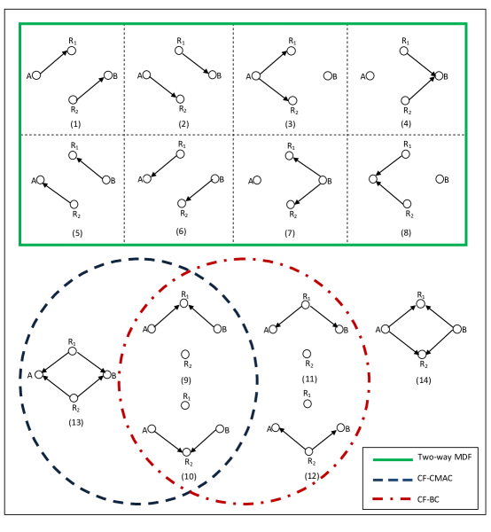
The diamond relay network has possible states, since each of the four half-duplex nodes can either be in transmit or receive state. Of these 16 states, we can ignore the 2 states in which all nodes are in transmit or all are in receive states, as they do not help in information flow. The 14 useful states are shown in Fig. 2. As an illustration, when state 14 is used, nodes and transmit symbols denoted and , and this is received as at and at with denoting additive noise. Specifying a relaying protocol involves specifying the sequence of states and the coding/decoding schemes for each of these states. In one-way communication over the diamond channel in [2], only states 1 to 4 need to be considered for communication from to . In two-way communication, all 14 states need to be considered in general.
As mentioned before, is the rate of communication from to and is the rate of communication from to . The capacity region for two-way communication consists of all pairs for which reliable two-way communication is possible.
III Capacity Region Outer Bound
In this section, we derive an outer bound to the capacity region of the two-way Gaussian diamond channel, which holds for any two-way relaying protocol. The bound is derived using the half-duplex cutset bound [12] and the boundary of this region can be computed by solving linear programs.
In general, we should consider all 14 states for deriving the outer bound. However, if a state has all cut capacities lesser than or equal to the corresponding cut capacities for another state, then only the state with higher cut capacities needs to be considered. In this network, 8 of the states (3,4 and 7-12) are dominated by either State 13 or 14. Therefore, we consider only the 6 states: 1, 2, 5, 6, 13, 14 with the fraction of time the network in state being denoted .
Theorem 1
Any achievable rate pair for two-way communication over the diamond channel must satisfy the following inequalities for some :
| (1) |
Proof:
For any general network with states and a fraction of time in state , any achievable rate of information flow is bounded as
| (2) |
where is the rate from source to destination node with the source in a subset of nodes and the destination in . The set defines a cut that separates source and destination. This bound is applied to the two-way diamond channel using the cuts ,,, for bounding and the cuts ,,, for bounding . Using these cuts, we obtain the following.
The mutual information terms in the above equations can be further bounded resulting in (1). For example, and [12, 11]. ∎
The boundary of the capacity region in Theorem 1 can be computed by solving the following linear program for each : subject to and the constraints in (1).
IV Proposed Protocols and Achievable Rates
IV-A Two-way MDF protocol
In [2], a multihopping-decode-and-forward (MDF) protocol is proposed for one way communication in the diamond channel. A simple two-way protocol can use the same MDF protocol for both flows ( to and to ) in a time-sharing manner. Thus, states 1-4 in Fig. 2 will be used for communication from to , and states 5-8 will be used for communication from to . We call this protocol that uses states 1-8 and a decode-and-forward (DF) strategy in each state as the two-way MDF protocol.
The maximum achievable rate for the one-way MDF protocol can be computed as in [2]. Suppose this rate for communication from to is and for communication from to is , then the achievable rate region for the two-way MDF protocol is the triangular region enclosed by the three straight lines: (1) , (2) , and (3) the line joining and .
IV-B CF-CMAC protocol
In this protocol, states 9, 10, and 13 are used. States 9 and 10 are multiple access channels (MACs), in which both the nodes and transmit to one of the relays. This protocol employs a compute and forward strategy at the relays, making use of doubly nested lattice codes following [6],[13] to decode the sum of the messages received from and , instead of decoding the individual messages. This sum is forwarded to the two nodes in state 13. State 13 is a Compound MAC (CMAC), in which both the relays simultaneously transmit to both nodes and . In a CMAC, each transmitter sends one message that should be decoded at both the receivers.
Doubly Nested Lattice codes
A nested lattice code is the set of all points of a fine lattice that are within the fundamental Voronoi region of a coarse lattice , i.e., . In [6], it was shown that, for every , there exist a sequence of -dimensional lattices , as , with second moments and such that the rate of the nested lattice code associated with the lattice partition , as , approaches
| (3) |
while the coding rate of the nested lattice code associated with the lattice partition , as , approaches
| (4) |
Using doubly nested lattice codes, an achievable rate region has been derived in [6] for the case of the Gaussian two-way relay channel. We use the same design for the states 9 and 10 of the CF-CMAC protocol. We provide a brief description for completeness, and refer to [6] for more details.
State 9
Consider an -dimensional doubly nested lattice code , with second moments and assuming . Node chooses a message , while chooses a message . The nodes and transmit
| (5) |
respectively, where are random dithers uniformly distributed in the Voronoi regions of and . Note that the transmit signals and are pre-divided by the respective channel gains to ensure that a noisy version of the sum is received at the relay. The relay receives
| (6) |
multiplies by the MMSE coefficient and subtracts the dithers to obtain
where
Here, denotes quantization to the nearest lattice point and is the effective noise at the relay with variance which results in higher effective SNR at the relay.
The relay attempts to decode by quantizing to the closest point in the fine lattice, and an error occurs if is outside the Voronoi region. The probability of error vanishes [13] as if the second moment satisfies
| (7) |
From (3), (4), (7), the rate constraints for State 9 can be written as follows.
| (8) |
where is the fraction of time for state 9, and denotes the amount of information flow from to in state .
State 10
State 10 follows a similar lattice coding scheme as State 9, possibly using a different doubly nested lattice code , with second moments and assuming . Nodes and choose messages , from , , and the relay decodes
| (9) |
where are random dithers. Proceeding as for state 9, the rate constraints for state 10 can be written as
| (10) |
State 13
In state 13, both the relays simultaneously transmit the decoded sum of messages to both nodes and . Both and are required to decode the message sent from each relay. Relay generates a Gaussian codebook consisting of -length sequences, with each element being i.i.d and having a Gaussian distribution . We assume that the relays make no error in decoding and in the first two states, which will be true if the rate constraints described above are satisfied. Since is uniformly distributed over , for every , the relay chooses to transmit a particular . Similarly, generates a random Gaussian codebook consisting of -length sequences, with each element being i.i.d and for every , the relay broadcasts a particular . This results in MACs at nodes and . Node receives from which it decodes and .
Since there is a one-to-one correspondence between the elements of and , can obtain from . Also, can obtain from because of the one-to-one correspondence between the elements of and . Similarly, can obtain and from the received vector
Since , are messages transmitted by to the relays in states 9 and 10, node has a priori knowledge of them. This can be used as side-information for decoding and . Using the knowledge of , can decode from as Using , can decode from as Similarly, using its a priori knowledge of , and dithers, node can decode and from and as
| (11) |
The rate constraints for correct CMAC decoding in state 13 are [14]:
| (12) |
| (13) |
| (14) |
where the last 2 constraints are the MAC constraints at and on the sum rates. Thus, this rate region is an intersection of the 2 MAC regions defined by the 2 receivers and .
Equating the information received at a relay from one node to the information forwarded by it to the other node, gives us the following four flow constraints.
| (15) |
The rates of information transfer between the end nodes and in the two directions are
| (16) |
In summary, the achievable rate region can be obtained by taking and solving the linear program with the rate constraints for states 9, 10 and 13, flow constraints (15) and , as constraints, for various values of .
IV-C CF-BC protocol
The CF-BC protocol uses states 9-12. Only one relay is used in any state. States 9 and 10 are used the same way as in the CF-CMAC protocol and have the same rate constraints. However, the computed sum of messages at each relay is forwarded to the 2 destinations in a time-shared manner, i.e., relay transmits to and using the broadcast state 11 and relay transmits to and using the broadcast state 12. The rate constraints for states 11 and 12 are:
| (17) |
| (18) |
IV-D Time-sharing between CF-CMAC and two-way MDF
The CF-CMAC protocol achieves some rate-pairs that the two-way MDF protocol cannot achieve. Time-sharing between CF-CMAC and two-way MDF can be used to achieve all convex combinations of rate-pairs achieved by the two protocols. Such a protocol would used states.
V Two-way Diamond Channel with Direct Source-Destination Link
In this Section, we consider the diamond network with a direct link between nodes and with SNR .
V-A Outer Bound
In Section III, 6 states were considered to obtain the outer bound. In this network with direct source-destination link, 10 states need to be considered for obtaining the outer bound. They are states 1-8, 13 and 14. Note that the - link should also be included in states 1-8. In states 13 and 14, the direct link does not play a role since nodes and are both transmitters or both receivers.
Theorem 2
Any achievable rate pair for two-way communication over the diamond channel with direct source-destination link must satisfy the following inequalities for some :
| (19) |
where the fraction of time network is in state is denoted .
V-B Achievable Rate Regions
The CF-CMAC and CF-BC protocols can be used for this network as well. Since nodes and are both transmitters or both receivers in the states used in the CF-BC and CF-CMAC protocols, the direct link does not affect the protocol and the achievable rate regions remain the same as in the case without the direct link.
The Cooperative Multiple Access Broadcast Channel (CoMABC) protocol proposed in [10] for two way relaying with one relay makes use of the direct link. This protocol is a three state protocol. The first state is a MAC where both end nodes and transmit to the relay. The second state is a broadcast from the relay. If the link to relay is better than the one from , then may transmit more bits in the first state and may receive at much lower rate in the second state. This is compensated using a third co-operative state after finishes decoding in the broadcast state. In the third state, and the relay together transmit to . may re-transmit some information to help in decoding, or may choose to transmit altogether new information. As in the CF-BC protocol, we now use the CoMABC protocol with either with or with depending on the rate pair to be achieved. We call this protocol the 2-relay CoMABC protocol.
Assuming that and , the 2-relay CoMABC protocol uses states 9, 11, 2 and 10, 12, 1. The achievable rate region is the closure of the set of all points satisfying following constraints:
| (20) |
where and the fraction of time the network is in state is denoted . When , state 6 is used instead of state 2 and a similar region can be obtained. Similarly, when , state 5 is used instead of state 1 and a similar region can be obtained.
VI Two-way Diamond Channel with Interfering Relays
In this Section, we consider the diamond network with a link between nodes and with SNR .
VI-A Outer Bound
In this network with interfering relays, 10 states need to be considered for obtaining the outer bound. They are states 1, 2, 5, 6, 9-14.
Theorem 3
Any achievable rate pair for two-way communication over the diamond channel with interfering relays must satisfy the following inequalities for some :
| (21) |
where the fraction of time network is in state is denoted .
VI-B Achievable Rate Regions
The CF-CMAC and CF-BC protocols can be used even in this case. The achievable rate region for these protocols remains the same as in the case without the - link, i.e., the CF-BC and CF-CMAC protocols do not use the link between the two relays.
Another achievable rate region for this channel using the - link can be obtained using States 1, 2, 5 and 6 by time-sharing the one-way alternating path relaying protocol in [15] between the two flows. We denote this protocol the 2-way AR-DF protocol. Consider the flow from to . In State 2, transmits to while transmits to . decodes the message from , and in addition decodes the message from too, considering it as data to be forwarded to in the next state. Thus, acts as a relay for both and . In state 1, transmits new information to , transmits to . The message transmitted by will be a combination of the messages received from and and the message to be sent to . States 5 and 6 act in the same way for the flow in the opposite direction, .
The achievable rate region for the 2-way AR-DF protocol is the closure of the set of all points satisfying following constraints [15]:
| (22) |
where the fraction of time in state is denoted .
VII Numerical Results and Comparisons
VII-A Diamond Channel
In this section, we compare the achievable rate regions of the two-way MDF, CF-BC, and CF-CMAC protocols and also compare with the capacity region outer bound. Numerical results are shown for three different channels: I, II, and III.
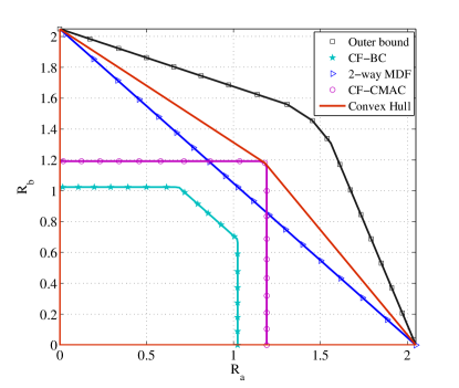
Figure 3 shows the comparison of rate regions for channel I. It has been shown in [2] that under this channel condition the one-way MDF protocol achieves capacity. Therefore, the two-way MDF region meets the outer bound on the axes where it corresponds to one-way MDF. However, away from the two axes, the two-way MDF has a significant gap from the outerbound. The CF-BC protocol, which uses one relay at a time, is not able to provide any improvement in this scenario. However, the proposed CF-CMAC protocol is able to achieve rate-pairs outside the rate region of the two-way MDF protocol. The convex combination of the CF-CMAC and two-way MDF protocol rate regions is also shown (labelled “convex hull”). Any point in this convex hull can be achieved by time-sharing the CF-CMAC and two-way MDF protocols.
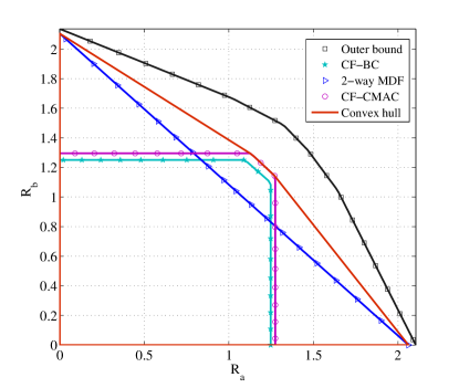
Figure 4 shows the comparison of rate regions for channel II. In this scenario, both the CF-BC and CF-CMAC protocols achieve rate-pairs outside the two-way MDF rate region. Even CF-BC, which selects one relay and uses compute-and-forward, provides gains in this case.
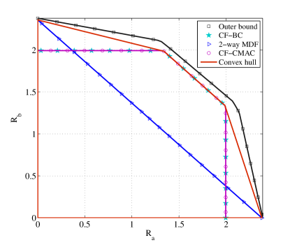
Figure 5 shows the comparison of rate regions for channel III. In this scenario, the links to relay are significantly better than the links to in terms of SNR. Therefore, this scenario is closer to a one-relay system. Both the CF-BC and CF-CMAC protocols achieve rate-pairs outside the two-way MDF rate region and close to the outer bound.
In general, the one-way MDF protocol is close to capacity for the one-way diamond channel. Therefore, by time-sharing, one can obtain rates close to capacity near the axes. However, when the desired two-way rates are nearly equal, time-sharing of one-way protocols is far from optimal, and the proposed CF-CMAC and CF-BC protocols achieve much better rates.
VII-B Diamond Channel with Direct Link
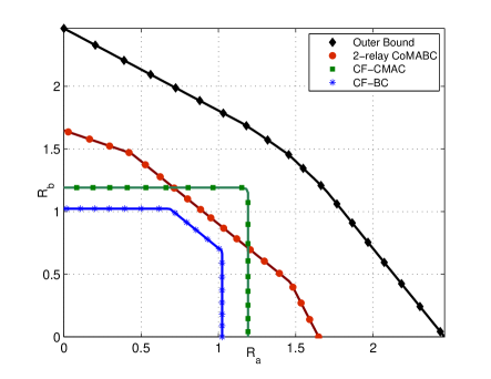
Figure 6 compares the achievable rate regions of the CF-BC, 2-relay CoMABC protocol, and CF-CMAC protocols with the outer bound. The 2-relay CoMABC protocol always achieves a larger rate region than the CF-BC protocol since it uses the direct link as well. The CF-CMAC can achieve some rate pairs that the 2-relay CoMABC cannot achieve even without using the direct link. This is because both relays transmit simultaneously in state 13 of the CF-CMAC protocol. Mixing of flows using the CF-CMAC protocol performs well for symmetric rates, while the 2-relay CoMABC protocol using the direct link performs better for asymmetric rates.
VII-C Diamond Channel with Interfering Relays
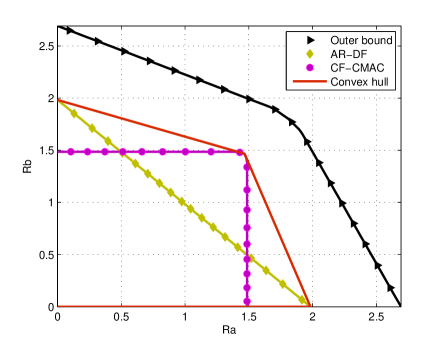
Figure 7 shows the achievable rate regions of the 2-way AR-DF and CF-CMAC protocols with the outer bound. The convex hull of the rates achieved by the CF-CMAC and 2-way AR-DF protocols is also shown. Again, mixing of flows using the CF-CMAC protocol performs well for symmetric rates, while the 2-way AR-DF protocol performs better for asymmetric rates. The AR-DF protocol could be further improved using the other one-way states 3, 4, 7, and 8.
VIII Conclusions
In this paper, we considered the Gaussian two-way diamond channel. We derived an outer bound for the capacity region and proposed relaying protocols based on the compute-and-forward technique. The proposed CF-CMAC protocol achieves rate-pairs that two-way protocols based on time-sharing or relay selection cannot achieve. There is still significant room for improving the achievable rates or the outer bound in several interesting channel conditions. The interference channel state (state 14 in Fig. 2) will probably play a vital role in closing the gap further.
We also considered the diamond channel with direct source-destination link and the diamond channel with interfering relays. We derived outer bounds for the capacity region in each case. We developed the 2-relay CoMABC protocol for the diamond channel with direct link and compared the achievable rate region with the CF-BC and CF-CMAC protocols and the outer bound. We also compared the 2-way AR-DF protocol with the CF-CMAC protocol and the outer bound for the diamond channel with interfering relays. As in the diamond channel, mixing the flows using compute and forward strategies is found to be important for symmetric rates.
References
- [1] B. Schein and R. Gallager, “The Gaussian parallel relay network,” in Proceedings of the IEEE International Symposium on Information Theory, 2000, p. 22.
- [2] H. Bagheri, A. Motahari, and A. Khandani, “On the capacity of the half-duplex diamond channel,” in Proceedings of the IEEE International Symposium on Information Theory, June 2010, pp. 649–653.
- [3] P. Popovski and H. Yomo, “Physical network coding in two-way wireless relay channels,” in IEEE ICC 2007, 2007, pp. 707–712.
- [4] S. Kim, P. Mitran, and V. Tarokh, “Performance bounds for bidirectional coded cooperation protocols,” IEEE Transactions on Information Theory, vol. 54, no. 11, pp. 5235–5241, Nov. 2008.
- [5] S. Kim, N. Devroye, P. Mitran, and V. Tarokh, “Achievable rate regions and performance comparison of half duplex bi-directional relaying protocols,” IEEE Transactions on Information Theory, vol. 57, no. 10, pp. 6405–6418, Oct. 2011.
- [6] W. Nam, S-Y.Chung, and Y. H. Lee, “Capacity of the Gaussian two-way relay channel to within 1/2 bit,” IEEE Transactions on Information Theory, vol. 56, pp. 5488–5494, Nov. 2010.
- [7] M. Wilson, K. Narayanan, H. Pfister, and A. Sprintson, “Joint physical layer coding and network coding for bidirectional relaying,” IEEE Trans. on Information Theory, vol. 56, no. 11, pp. 5641–5654, Nov. 2010.
- [8] B. Nazer and M. Gastpar, “Compute-and-forward: Harnessing interference through structured codes,” IEEE Transactions on Information Theory, vol. 57, no. 10, pp. 6463–6486, Oct. 2011.
- [9] C. Gong, G. Yue, and X. Wang, “A transmission protocol for a cognitive bidirectional shared relay system,” IEEE Journal of Selected Topics in Signal Processing, vol. 5, no. 1, pp. 160–170, Feb. 2011.
- [10] Y. Tian, D. Wu, C. Yang, and A. Molisch, “Asymmetric two-way relay with doubly nested lattice codes,” IEEE Transactions on Wireless Communications, vol. 11, no. 2, pp. 694–702, Feb. 2012.
- [11] I. Ashar, V. Prathyusha, S. Bhashyam, and A. Thangaraj, “Outer bounds for the capacity region of a Gaussian two-way relay channel,” in Allerton Conference on Communication, Control, and Computing, Monticello, IL, USA, Oct. 2012.
- [12] M. Khojastepour, A. Sabharwal, and B. Aazhang, “On capacity of Gaussian‘cheap’relay channel,” in IEEE Global Telecommunications Conference, 2003., vol. 3. IEEE, 2003, pp. 1776–1780.
- [13] W. Nam, S.-Y. Chung, and Y. Lee, “Nested lattice codes for Gaussian relay networks with interference,” IEEE Transactions on Information Theory, vol. 57, no. 12, pp. 7733–7745, Dec. 2011.
- [14] R. Ahlswede, “The capacity region of a channel with two senders and two receivers,” Annals of Probability, vol. 2, no. 5, pp. 805–814, Oct. 1974.
- [15] W. Chang, S.-Y. Chung, and Y. H. Lee, “Capacity Bounds for Alternating Two-Path Relay Channels,” in Allerton Conference on Communication, Control, and Computing, Monticello, IL, USA, Sep. 2007.