Chemical abundances in the extremely Carbon and Xenon-rich halo planetary nebula H4-1

Abstract

We performed detailed chemical abundance analysis of the extremely metal-poor ([Ar/H]$\sim$–2) halo planetary nebula H4-1 based on the multi-wavelength spectra from Subaru/HDS, $GALEX$, $SDSS$, and $Spitzer$/IRS and determined the abundances of 10 elements. The C and O abundances were derived from collisionally excited lines (CELs) and are almost consistent with abundances from recombination lines (RLs). We demonstrated that the large discrepancy in the C abundance between CEL and RL in H4-1 can be solved using the temperature fluctuation model. We reported the first detection of the [Xe iii]$\lambda$5846 Å line in H4-1 and determination of its elemental abundance ([Xe/H]$>$+0.48). H4-1 is the most Xe-rich PN among the Xe-detected PNe. The observed abundances are close to the theoretical prediction by a $\sim$2.0 $M_{\odot}$ single star model with initially $r$-process element rich ([$r$/Fe]=+2.0 dex). The observed Xe abundance would be a product of the $r$-process in primordial SNe. The [C/O]-[Ba/(Eu or Xe)] diagram suggests that the progenitor of H4-1 shares the evolution with two types of carbon-enhanced metal-poor stars (CEMP), CEMP-$r$/$s$ and CEMP-$no$ stars. The progenitor of H4-1 is a presumably binary formed in an $r$-process rich environment.

1. Introduction

Currently, more than 1000 objects are considered planetary nebulae (PNe) in the Galaxy, about 14 of which have been identified as halo members because of their current location and kinematics (e.g., Otsuka et al., 2008a). Halo PNe are interesting objects because they provide direct insight into the final evolution of old, low-mass metal-poor halo stars.

The halo PN H4-1 is extremely metal-poor ($Z$$\sim$10^-4, [Fe/H]=–2.3) and C-rich (Torres-Peimbert & Peimbert, 1979; Kwitter et al., 2003), similar to the C-rich halo PNe BoBn1 in the Sagittarius dwarf spheroidal galaxy (Otsuka et al., 2010, 2008a) and K648 in M15 (Rauch et al., 2002). The chemical abundances and metallicity of these three PNe imply that their progenitors formed early, perhaps $\sim$10-13 Gyrs ago. However, these extremely metal-poor halo PNe have an unresolved issue: how did their progenitors evolve into C-rich PNe?

The initial mass of these three PNe is generally thought to equal $\sim$0.8 $M_{\odot}$, which corresponds to the turn-off stellar mass of M15. According to recent stellar evolution models (e.g., Lugaro et al., 2012; Fujimoto et al., 2000), there are two mechanisms for stars with $Z$$\lesssim$10^-4 to become C-rich: (1) helium-flash driven deep mixing (He-FDDM) for $<$2.5-3 $M_{\odot}$ stars and (2) third dredge-up (TDU) for $\gtrsim$0.9-1.5 $M_{\odot}$ stars. Mechanism (1) is unlikely for these PNe because this mechanism occurs in stars with $Z$$\lesssim$6$\times$10^-5 ([Fe/H]$\lesssim$–2.5). Therefore, TDU is essential for these PNe to become C-rich, implying that it is possible that these halo PNe evolved from $\gtrsim$0.8-0.9 $M_{\odot}$ single stars. We should note that the lower limit mass required for TDU depends largely on models. The minimum mass for the occurrence of the TDU is thought to be 1.2-1.5 $M_{\odot}$ (e.g., Lattanzio, 1987; Boothroyd & Sackmann, 1988).

Even if the progenitor of H4-1 is a $\gtrsim$0.8-0.9 $M_{\odot}$ single star and it experienced TDU during AGB phase, current low-mass stellar evolution models are unlikely to explain the evolution of H4-1; the effective temperature of the central star of H4-1 is between 93 400 (Mal’Kov, 1997) and 132 000 K (Henry et al., 1996), and the age of the PN is 8400 yrs, assuming a distance of 25.3 kpc from us (Mal’Kov, 1997). The He-shell burning model for the initially 0.89 $M_{\odot}$ and $Z$=0.004 stars by Vassiliadis & Wood (1994) predicted that it takes $>$50 000 yrs for a star to reach 10⁵ K. There is obviously a large discrepancy in evolutional time scale between the observations and theoretical models.

To explain the evolution of H4-1, we need to consider additional mechanisms that shorten the evolutionary timescale, e.g., binary mass-transfer via Roche lobe overflow, which was proposed for BoBn1 by Otsuka et al. (2010). Evidence suggests that binary evolution is the most plausible scenario for H4-1. In particular, Tajitsu & Otsuka (2004) showed that H4-1 has a bright equatorial disk, a bipolar nebula, and multiple arcs in its molecular hydrogen image. The discovery of these structures implies that H4-1 would have evolved from a binary, similar to carbon-enhanced metal-poor (CEMP) stars found in the Galactic halo and these CEMP stars show [Fe/H]$<$–2 (see Beers & Christlieb, 2005). Otsuka et al. (2008b) found that the location of H4-1 on [C/(Fe or Ar)] versus [(Fe or Ar)/H] diagrams is in the region occupied by CEMP stars, indicating a similar origin and evolution.

Elements with atomic number $Z$$>$30 are synthesized in the neutron ($n$) capturing process in both PN progenitors and supernovae (SNe). In PN progenitors, the $n$-flux is much lower, so the $n$-capturing process is a slow process ($s$-process). In SNe, because of a much higher $n$-flux, the $n$-capturing process is a rapid process ($r$-process). Several types of CEMP stars show the enhancements of $s$- and/or $r$-process elements. Therefore, if we can detect any $n$-capture elements, we would be able to obtain important insights into the evolution of H4-1 and the chemical environment where its progenitor was born by comparing the carbon and $n$-capture elements of H4-1 and those of CEMP stars.

The elements C and O are clearly important with respect to the evolution of H4-1. However, there is a large discrepancy in the C abundances between collisionally excited lines (CELs) and recombination lines (RLs). Torres-Peimbert & Peimbert (1979) estimated the C number density using RLs and found that log $n$(C)/$n$(H)+12=9.39, whereas Henry et al. (1996) found a value of 8.68 using CELs. Discrepancies in C and O abundances have already been found in many Galactic PNe (e.g., Liu, 2006). It is necessary to solve the C discrepancy in H4-1 (the O discrepancy, too if exist).

In this paper, we report a detail chemical abundance analysis of H4-1 based on deep high-dispersion optical spectra from Subaru/HDS, and archived UV, optical, and mid-IR spectra from $GALEX$, the Sloan Digital Sky Survey (SDSS), and $Spitzer$/IRS, respectively. In Section 2, we describe the observations. In Section 3, we provide the ionic and elemental abundances of H4-1 derived from CELs and RLs. The first detection of the $n$-capture element xenon (Xe) is reported in this section. In Section 4.1, we discuss the discrepancy in C and O abundances. In Sections 4.2 and 4.3, we discuss the Xe abundance by comparing with the theoretical nucleosynthesis model and the origin and evolution of H4-1 from the view point of chemical abundances. A summary is given in Section 5.

2. Observations & Data Reduction

2.1. HDS observations

Figure 1.— The de-reddened HDS spectrum of H4-1. The wavelength is shifted to the rest wavelength in air.

Table 1Detected lines and identifications of H4-1 in HDS spectra.

$\lambda_{\rm obs}$	Ion	$\lambda_{\rm lab}$	Comp.	$f$($\lambda$)	$I$($\lambda$)	$\delta$$I$($\lambda$)
(Å)		(Å)
3667.25	H25	3669.46	1	0.334	0.355	0.047
3669.30	H24	3671.48	1	0.333	0.386	0.058
3671.53	H23	3673.74	1	0.333	0.439	0.096
3672.35	He ii	3674.84	1	0.333	0.177	0.054
3674.11	H22	3676.36	1	0.332	0.584	0.066
3677.16	H21	3679.35	1	0.332	0.564	0.061
3680.61	H20	3682.81	1	0.331	0.672	0.052
3684.64	H19	3686.83	1	0.330	0.906	0.069
3689.34	H18	3691.55	1	0.329	0.911	0.062
3694.92	H17	3697.15	1	0.328	1.175	0.075
3701.62	H16	3703.65	1	0.327	1.316	0.073
3702.81	He i	3704.98	1	0.327	0.647	0.047
3704.95	O iii	3707.25	1	0.326	0.056	0.038
3709.73	H15	3711.97	1	0.325	1.513	0.075
3712.80	O iii	3715.08	1	0.325	0.085	0.028
3719.69	H14	3721.94	1	0.323	1.971	0.090
3723.63	[O ii]	3726.03	1	0.322	50.749	2.492
3723.94	[O ii]	3726.03	2	0.322	40.319	2.203
			Tot.		91.068	3.326
3726.33	[O ii]	3728.81	1	0.322	42.426	1.851
3726.69	[O ii]	3728.81	2	0.322	42.795	1.841
			Tot.		85.221	2.610
3730.62	He i	3732.86	1	0.321	0.103	0.031
3732.12	H13	3734.37	1	0.321	2.465	0.109
3747.89	H12	3750.15	1	0.317	2.991	0.125
3752.40	O iii	3754.70	1	0.316	0.182	0.020
3768.37	H11	3770.63	1	0.313	3.775	0.155
3795.61	H10	3797.90	1	0.307	4.840	0.194
3817.34	He i	3819.60	1	0.302	1.238	0.054
3831.40	He i	3833.55	1	0.299	0.128	0.030
3833.08	H9	3835.38	1	0.299	7.301	0.286
3855.71	He ii	3858.07	1	0.294	0.105	0.024
3865.16	He i	3867.47	1	0.291	0.136	0.021
3866.44	[Ne iii]	3868.77	1	0.291	5.323	0.225
3869.43	He i	3871.83	1	0.290	0.091	0.020
3886.73	H8	3889.05	1	0.286	9.712	0.387
3918.27	C ii	3920.68	1	0.279	0.050	0.018
3921.09	He ii	3923.48	1	0.278	0.124	0.016
3924.18	He i	3926.54	1	0.277	0.111	0.014
3962.36	He i	3964.73	1	0.267	0.658	0.036
3965.08	[Ne iii]	3967.46	1	0.267	1.562	0.059
3966.01	He ii	3968.43	1	0.266	0.170	0.020
3967.68	H7	3970.07	1	0.266	14.235	0.506
4006.90	He i	4009.26	1	0.256	0.191	0.021
4023.81	He i	4026.18	1	0.251	1.969	0.068
4065.47	C iii	4067.87	1	0.239	0.162	0.015
4066.40	[S ii]	4068.60	1	0.239	0.277	0.019
4067.77	O ii	4070.14	1	0.239	0.261	0.018
4089.64	O ii	4092.93	1	0.232	0.043	0.019
4094.83	N iii	4097.35	1	0.231	0.283	0.016
4097.54	He ii	4100.04	1	0.230	0.249	0.039
4099.27	H6	4101.73	1	0.230	25.395	0.781
4100.90	N iii	4103.39	1	0.229	0.231	0.028
4118.37	He i	4120.81	1	0.224	0.269	0.026
4126.21	[Fe ii]	4128.75	1	0.222	0.077	0.024
4141.30	He i	4143.76	1	0.217	0.320	0.020
4197.27	He ii	4199.83	1	0.200	0.378	0.014
4264.60	C ii	4267.15	1	0.180	1.118	0.035
4336.02	He ii	4338.67	1	0.157	0.393	0.070
4337.85	H5	4340.46	1	0.157	46.910	1.069
4346.71	O ii	4349.43	1	0.154	0.028	0.006
4360.52	[O iii]	4363.21	1	0.149	3.677	0.167
4360.58	[O iii]	4363.21	2	0.149	6.078	0.159
			Tot.		9.755	0.231
4385.32	He i	4387.93	1	0.142	0.532	0.016
4387.89	C iii	4390.50	1	0.141	0.071	0.020
4434.94	He i	4437.55	1	0.126	0.083	0.017
4468.83	He i	4471.47	1	0.115	4.487	0.093
4558.82	Mg i]	4562.60	1	0.087	0.031	0.007
4631.33	N iii	4634.12	1	0.065	0.083	0.011
4635.99	O ii	4638.86	1	0.064	0.057	0.006
4637.80	N iii	4640.64	1	0.063	0.148	0.006
4639.03	O ii	4641.81	1	0.063	0.047	0.005
4644.57	C iii	4647.42	1	0.061	0.232	0.007

Table 2Continued.

$\lambda_{\rm obs}$	Ion	$\lambda_{\rm lab}$	Comp.	$f$($\lambda$)	$I$($\lambda$)	$\delta$$I$($\lambda$)
(Å)		(Å)
4647.39	C iii	4650.25	1	0.060	0.147	0.006
4648.66	O ii	4651.33	1	0.060	0.024	0.005
4655.58	C iv	4658.20	1	0.058	0.065	0.004
4658.89	O ii	4661.63	1	0.057	0.035	0.005
4682.60	He ii	4685.68	1	0.050	4.491	0.109
4682.91	He ii	4685.68	2	0.050	13.819	0.199
			Tot.		18.310	0.227
4708.49	[Ar iv]	4711.37	1	0.042	0.065	0.007
4710.36	He i	4713.17	1	0.042	0.554	0.013
4737.32	[Ar iv]	4740.17	1	0.034	0.059	0.004
4856.37	He ii	4859.32	1	0.001	0.873	0.017
4858.37	H4	4861.33	1	0.000	42.807	1.844
4858.43	H4	4861.33	2	0.000	57.193	1.731
			Tot.		100.000	2.529
4919.00	He i	4921.93	1	–0.016	1.006	0.017
4928.29	[O iii]	4931.80	1	–0.019	0.073	0.013
4955.89	[O iii]	4958.91	1	–0.026	112.614	2.513
4955.96	[O iii]	4958.91	2	–0.026	111.463	1.811
			Tot.		224.077	3.097
5003.67	[O iii]	5006.84	1	–0.038	76.548	18.101
5003.85	[O iii]	5006.84	2	–0.038	578.884	17.282
5004.51	[O iii]	5006.84	3	–0.038	12.015	7.893
			Tot.		667.447	26.242
5012.69	He i	5015.68	1	–0.040	1.907	0.035
5028.99	C ii	5032.07	1	–0.044	0.044	0.008
5032.83	[Fe ii]	5035.48	1	–0.045	0.030	0.005
5044.74	He i	5047.74	1	–0.048	0.153	0.007
5124.28	Fe iii	5127.39	1	–0.066	0.018	0.004
5127.90	C iii	5130.86	1	–0.067	0.079	0.004
5137.51	C ii	5140.79	1	–0.069	0.046	0.009
5194.45	[N i]	5197.900	1	–0.082	0.144	0.009
5195.10	[N i]	5197.90	2	–0.082	0.366	0.010
			Tot.		0.510	0.013
5196.81	[N i]	5200.26	1	–0.083	0.117	0.008
5197.45	[N i]	5200.26	2	–0.083	0.315	0.012
			Tot.		0.432	0.015
5339.16	C ii	5342.19	1	–0.112	0.078	0.008
5339.19	C ii	5342.43	1	–0.112	0.082	0.014
5408.25	He ii	5411.52	1	–0.126	1.119	0.024
5514.37	[Cl iii]	5517.66	1	–0.145	0.062	0.007
5534.55	[Cl iii]	5537.60	1	–0.149	0.062	0.007
5573.87	[O i]	5577.34	1	–0.156	0.046	0.014
5574.30	[O i]	5577.34	2	–0.156	0.075	0.011
			Tot.		0.120	0.018
5751.02	[N ii]	5754.64	1	–0.185	0.588	0.031
5751.37	[N ii]	5754.64	2	–0.185	0.903	0.030
			Tot.		1.491	0.043
5797.75	C iv	5801.34	1	–0.192	0.060	0.007
5843.18	[Xe iii]	5846.67	1	–0.199	0.047	0.008
	+ He ii
5872.14	He i	5875.62	1	–0.203	14.918	0.363
6070.48	He ii	6074.30	1	–0.232	0.033	0.022
6147.72	C ii	6151.27	1	–0.242	0.059	0.009
6166.94	He ii	6170.69	1	–0.245	0.056	0.010
6230.09	He ii	6233.82	1	–0.254	0.023	0.009
6296.11	[O i]	6300.30	1	–0.263	1.198	0.038
6296.64	[O i]	6300.30	2	–0.263	0.520	0.113
6296.87	[O i]	6300.30	3	–0.263	4.681	0.177
			Tot.		6.399	0.214
6307.03	He ii	6310.85	1	–0.264	0.050	0.010
6308.17	[S iii]	6312.10	1	–0.264	0.106	0.013
6359.54	[O i]	6363.78	1	–0.271	0.377	0.016
6359.98	[O i]	6363.78	2	–0.271	0.134	0.041
6360.30	[O i]	6363.78	3	–0.271	1.602	0.064
			Tot.		2.114	0.077
6402.47	He ii	6406.38	1	–0.277	0.079	0.008
6457.98	N ii	6461.71	1	–0.284	0.134	0.011
6523.13	He ii	6527.10	1	–0.293	0.091	0.011
6543.91	[N ii]	6548.04	1	–0.296	8.636	0.348
6544.38	[N ii]	6548.04	2	–0.296	19.071	0.623
			Tot.		27.707	0.714
6556.05	He ii	6560.10	1	–0.297	0.710	0.083
6556.16	He ii	6560.10	2	–0.297	1.142	0.068
			Tot.		1.852	0.107

Table 2Continued.

$\lambda_{\rm obs}$	Ion	$\lambda_{\rm lab}$	Comp.	$f$($\lambda$)	$I$($\lambda$)	$\delta$$I$($\lambda$)
(Å)		(Å)
6558.82	H3	6562.77	1	–0.298	96.472	4.710
6558.87	H3	6562.77	2	–0.298	188.528	6.350
			Tot.		285.000	7.906
6574.09	C ii	6578.05	1	–0.300	0.376	0.015
6579.25	[N ii]	6583.46	1	–0.300	25.484	0.965
6579.73	[N ii]	6583.46	2	–0.300	55.214	1.775
			Tot.		80.697	2.021
6674.13	He i	6678.15	1	–0.313	1.805	0.070
6674.18	He i	6678.15	2	–0.313	1.596	0.056
			Tot.		3.401	0.090
6712.27	[S ii]	6716.44	1	–0.318	0.270	0.021
6712.70	[S ii]	6716.44	2	–0.318	0.235	0.018
			Tot.		0.505	0.028
6726.50	[S ii]	6730.81	1	–0.320	0.170	0.014
6727.02	[S ii]	6730.81	2	–0.320	0.408	0.018
			Tot.		0.577	0.023
6886.73	He ii	6890.90	1	–0.341	0.132	0.008
7061.04	He i	7065.18	1	–0.364	4.345	0.160
7071.72	[Xe v]?	7076.80	1	–0.366	0.020	0.007
7104.53	[K iv]	7108.90	1	–0.370	0.015	0.009
7111.35	C ii	7115.60	1	–0.371	0.020	0.007
7131.50	[Ar iii]	7135.80	1	–0.374	0.348	0.016
7156.36	He i	7160.61	1	–0.377	0.050	0.012
7173.17	He ii	7177.52	1	–0.379	0.112	0.007
7226.94	C ii	7231.34	1	–0.387	0.154	0.015
7232.09	C ii	7236.42	1	–0.387	0.345	0.017
7277.06	He i	7281.35	1	–0.393	0.535	0.062
7285.33	[Rb v]?	7289.81	1	–0.394	0.021	0.005
7293.77	He i	7298.04	1	–0.395	0.020	0.006
7314.87	[O ii]	7319.25	1	–0.398	0.933	0.058
7315.51	[O ii]	7319.89	1	–0.398	0.772	0.085
7315.99	[O ii]	7320.37	2	–0.398	2.193	0.108
			Tot.		2.965	0.137
7325.26	[O ii]	7329.65	1	–0.400	0.753	0.064
7325.55	[O ii]	7329.94	2	–0.400	0.819	0.050
			Tot.		1.572	0.082
7326.40	[O ii]	7330.79	1	–0.400	0.703	0.053
7326.62	[O ii]	7331.01	2	–0.400	0.648	0.038
			Tot.		1.351	0.065
7342.94	[V  ii]	7347.74	1	–0.402	0.057	0.010
7361.03	O iii	7365.35	1	–0.404	0.041	0.009
7369.17	[V  ii]	7373.32	1	–0.406	0.056	0.008
7373.23	[Ni ii]	7377.83	1	–0.406	0.026	0.011

The spectra of H4-1 were taken using the High-Dispersion Spectrograph (HDS; Noguchi et al., 2002) attached to one of the two Nasmyth foci of the 8.2-m Subaru telescope (Program ID: S09A-163S, PI: M.Otsuka).

The red spectra (4600-7500 Å) were obtained in May 2009, when weather conditions were unfavorable; there were scattered cirrus clouds in the sky and a full moon. The seeing was $\sim$1.5^′′ from the guider CCD. An atmospheric dispersion corrector (ADC) was used to minimize the differential atmospheric dispersion through the broad wavelength region. We set the slit width to equal $1.^{\prime\prime}5$ and chose a 2$\times$2 on-chip binning. We set the slit length to $7^{\prime\prime}$, which fit the nebula and allowed a direct subtraction of sky background from the object frames. The CCD sampling pitch along the slit length projected on the sky equaled $\sim 0.^{\prime\prime}276$ per a binned pixel. The resolving power reached approximately $R$ $>$33 000, which is derived from the mean full width at half maximum (FWHM) of narrow Th-Ar comparisons and night sky lines. We took a series of 1800 s exposures and the total exposure time was 12 600 s (7 exposure frames). In addition, we took a series of four 300 s exposures to measure the fluxes of strong lines such as [O iii]$\lambda$5007. For the flux calibration, blaze function correction, and airmass correction, we observed the standard star Hz44 three times at different airmasses.

The blue spectra (3600-5400 Å) were obtained in July 2009 using the same settings employed in the May 2009 observations, except for the slit width ($1.^{\prime\prime}2$). The seeing during these observations was 0.62^′′. We took four 1800 s exposure frames on 4 July and a single 600 s frame on 9 July.

Data reduction and emission line analysis were performed mainly with the long-slit reduction package noao.twodspec in IRAF. The resulting signal-to-noise (S/N) ratios at the peak of the detected emission lines in the spectra were $>$5 after subtracting the sky background, whereas that at the continuum was $>$40 at the blue spectrum and $>$50 at the red spectrum before subtracting the sky, even at the edges of each echelle order.

The line were de-reddened using the formula: $I$($\lambda$) = $F$($\lambda$)$\times$10^c(Hβ)f(λ), where $I$($\lambda$) is the de-reddened line flux, $F$($\lambda$) is the observed line flux, $f$($\lambda$) is the interstellar extinction parameter at $\lambda$ computed by the reddening law of Cardelli et al. (1989) with $R_{V}$=3.1, and $c$(H$\beta$) is the reddening coefficient at H$\beta$, respectively. The values of $F$(H$\beta$) were 1.85$\times$10^-13 $\pm$ 8.49$\times$10^-15 in blue and 2.13$\times$10^-13 $\pm$ 4.60$\times$10^-15 erg s^-1 cm^-2 in red. Hereafter, X(–Y) means X$\times$10^-Y. We measured $c$(H$\beta$) by comparing the observed Balmer line ratios of H$\gamma$ (blue spectrum) or H$\alpha$ (red spectrum) to H$\beta$ with the theoretical ratio of Storey & Hummer (1995), assuming the electron temperature $T_{\epsilon}$=10⁴ K and the electron density $n_{\epsilon}$=10⁴ cm^-3 in the Case B assumption. The value of $c$(H$\beta$) was 0.07$\pm$0.05 for the blue spectra and 0.11$\pm$0.04 for the red spectra.

Flux scaling was performed using all of the emission lines detected in the overlap region between the blue and the red spectra. The de-reddened fluxes relative to $I$(H$\beta$)=100 in both spectra are coincident within 11$\%$ of each other. The combined de-reddened spectrum is presented in Fig. 1. The observed wavelength at the time of observation was corrected to the averaged line-of-sight heliocentric radial velocity of –181.35$\pm$0.35 km s^-1 (root-mean-square of the residuals: 4.00 km s^-1) among over 120 lines detected in the HDS spectrum.

The detected lines are listed in Table 1. To ensure accuracy in the identification, we checked the presence of all of the detected lines and removed ghost emissions in the two-dimensional spectra. When measuring fluxes of the emission lines, we assumed that the line profiles were all Gaussian and we applied multiple Gaussian fitting techniques. We listed the observed wavelength and de-reddened relative fluxes of each Gaussian component (indicated by Comp.ID number in the fourth column of Table 1) with respect to the de-reddened H$\beta$ flux of 100. The line-profiles of most the detected lines can be fit by a single Gaussian component. For the lines composed of multiple components (e.g., [O ii]$\lambda$3726.03 Å), we list the de-reddened relative fluxes of each component and list the sum of these components (indicated by Tot.) in the last line.

2.2. The total H$\beta$ flux

To normalize the line fluxes relative to $F$(H$\beta$) in the $GALEX$ and $Spitzer$/IRS spectra, the $F$(H$\beta$) of the whole nebula is needed.

A measurement of $F$(H$\beta$)=3.16(–13) erg s^-1 cm^-2 was taken for the entire nebula by Kwitter et al. (2003) using a slit width of 5″. They also determined $c$(H$\beta$)=0.10.

The SDSS spectrum for H4-1 (SDSS; Object ID: 631018077386964992) provides another measurement, taken using a 3″ diameter optical fiber. A total H$\beta$ flux of 4.57(–13)$\pm$3.13(–15) erg s^-1 cm^-2 was measured by applying an aperture correction factor of 2.07, which is listed in the SDSS webpage and is from the $r$-band flux ratio between the image and the fiber spectra. A value of $c$(H$\beta$)=0.10$\pm$0.04 was derived by comparing the observed $F$(H$\beta$)/$F$(H$\gamma$) ratio to the theoretical value for the case of $T_{\epsilon}$=10⁴ K and $n_{\epsilon}$=10⁴ cm^-3, because the H$\alpha$ line was saturated.

We used a H$\beta$ flux value of 3.86(–13) erg s^-1 cm^-2, which is the average between the values from the SDSS and Kwitter et al. (2003).

2.3. GALEX archive data

Table 3The detected lines in the $GALEX$ spectra.

$\lambda_{\rm lab}$	Ion	$f$($\lambda$)	$F$($\lambda$)a	$I$($\lambda$)
(Å)			(erg s-1 cm-2)	[$I$(H$\beta$)=100]
1549/51	C iv	1.238	1.32(–12)$\pm$5.36(–14)	3.42(+2)$\pm$1.89(+1)
1640	He ii	1.177	4.87(–13)$\pm$4.38(–14)	1.26(+2)$\pm$1.23(+1)
1660/66	$[$O iii$]$	1.167	2.10(–13)$\pm$7.83(–14)	5.43(+1)$\pm$2.04(+1)
1906/09	C iii$]$	1.257	6.04(–12)$\pm$7.73(–14)	1.56(+3)$\pm$6.18(+1)
2326	$[$C ii$]$	1.364	1.68(–12)$\pm$1.86(–14)	4.35(+2)$\pm$1.70(+1)
2470	$[$O ii$]$	1.045	1.94(–14)$\pm$7.00(–15)	5.10(0)$\pm$1.82(0)

We analyzed the Galaxy Evolution Explorer ($GALEX$; Martin et al., 2005) slit-less prism spectra to estimate the CEL C^+,2+,3+ and O⁺ abundances using the [C ii] $\lambda$2326 Å, C iii$]$ $\lambda$1906/09 Å, C iv $\lambda$1549/51 Å, and [O ii] $\lambda$2470 Å lines. The GALEX spectra were retrieved from the multi-mission archive at the STScI (MAST; GALEX Object ID: 2555724756316858403). We used both FUV (1344-1786 Å) and NUV (1771-2831 Å) band spectra. We did not correct the reddening because the observed flux ratio of He ii $F$(1640 Å)/$F$(4686 Å) = 6.88$\pm$0.62 was comparable to the theoretical ratio of He ii $I$($\lambda$1640)/($\lambda$4686)=6.56 in the case of $T_{\epsilon}$=10⁴ K and $n_{\epsilon}$=10⁴ cm^-3 as given by Storey & Hummer (1995).

The observed and normalized fluxes of the detected lines are listed in Table 3.

2.4. $Spitzer$/IRS archive data

Table 4The detected atomic lines in the $Spitzer$ spectra.

$\lambda_{\rm lab}$	Ion	$f$($\lambda$)	$F$($\lambda$)a	$I$($\lambda$)
($\mu$m)			(erg s-1 cm-2)	[$I$(H$\beta$)=100]
10.51	[S iv]	–0.960	4.97(–15)$\pm$4.06(–16)	1.21$\pm$0.15
12.40	H i	–0.980	4.33(–15)$\pm$3.94(–16)	1.04$\pm$0.13
12.81	[Ne ii]	–0.983	1.62(–15)$\pm$1.85(–16)	0.39$\pm$0.06
15.56	[Ne iii]	–0.985	1.48(–14)$\pm$3.89(–16)	3.56$\pm$0.34
16.12	He i	–0.984	3.08(–15)$\pm$2.36(–16)	0.74$\pm$0.09
17.63	He i	–0.981	6.12(–15)$\pm$6.05(–16)	1.47$\pm$0.20
18.71	[S iii]	–0.981	3.80(–15)$\pm$2.34(–16)	0.91$\pm$0.10
25.89	[O iv]	–0.989	1.29(–13)$\pm$8.57(–16)	30.87$\pm$2.84

The spectra were taken on June 12, 2007 using the Infrared Spectrograph ($IRS$; Houck et al., 2004) with the SL (5.2-14.5 $\mu$m), SH (9.9-19.6 $\mu$m), and LH (18.7-37.2 $\mu$m) modules (AOR Keys: 18628864 and 186291202; PI: J. Bernard-Salas). We used the reduction package SMART v.8.2.5 provided by the IRS team at Cornell University (Higdon et al., 2004) and IRSCLEAN provided by the $Spitzer$ Science Center. For SH and LH spectra, we subtracted the sky background using off-set spectra. We scaled the SL data up to SH&LH in the overlapping wavelength region, and then re-scaled the scaled 5.2-37.2 $\mu$m to match the Wide-field Infrared Survey Explorer ($WISE$) bands 3 ($\lambda_{c}$=11.56 $\mu$m) and 4 ($\lambda_{c}$=22.09 $\mu$m) average flux densities (1.91(–13) erg s^-1 cm^-2 $\mu$m^-1 in band 3 and 3.16(–13) erg s^-1 cm^-2 $\mu$m^-1 in band 4).

The line fluxes of detected atomic lines are listed in Table 4. We derived $c$(H$\beta$)=0.03$\pm$0.04 by comparing the observed intensity ratio of H i $F$(12.4 $\mu$m)/$F$(H$\beta$) to the theoretical value of Storey & Hummer (1995) for the case of $T_{\epsilon}$=10⁴ K and $n_{\epsilon}$=10⁴ cm^-3 (1.04). The line at 12.4 $\mu$m is the complex of H i $n$=9-7, and $n$=11-8. We used the interstellar extinction function given by Fluks et al. (1994).

3. Results

3.1. CELs Diagnostics

Figure 2.— $n_{\epsilon}$-$T_{\epsilon}$ diagram. Each curve is labeled with an ID number given in Table 5. The solid lines indicate diagnostic lines of the $T_{\epsilon}$. The broken lines indicate diagnostic lines of the $n_{\epsilon}$.

Table 5Plasma Diagnostics.

Parameters	ID	Diagnostic	Ratio	Result
$T_{\epsilon}$	(1)	$[$O ii$]$($\lambda$3726+$\lambda$3729)/($\lambda$7320+$\lambda$7330)	26.459$\pm$1.051a	12000$\pm$330
(K)	(2)	$[$S iii$]$($\lambda$18.7$\mu$m)/($\lambda$9531)	0.364$\pm$0.099	12 600$\pm$2200
	(3)	$[$Ne iii$]$($\lambda$15.5$\mu$m)/($\lambda$3869+$\lambda$3967)	0.518$\pm$0.052	13 400$\pm$500
	(4)	$[$O iii$]$($\lambda$4959+$\lambda$5007)/($\lambda$4363)	91.390$\pm$3.465	13 280$\pm$200
	(5)	$[$N ii$]$($\lambda$6548+$\lambda$6583)/($\lambda$5755)	72.701$\pm$2.541	11 300$\pm$180
	(6)	$[$O i$]$($\lambda$6300+$\lambda$6363)/($\lambda$5577)	70.704$\pm$10.527	9490$\pm$510
		He i($\lambda$7281)/($\lambda$6678)	0.157$\pm$0.019	7430$\pm$2190
		(Balmer Jump)/(H 11)	0.103$\pm$0.205	11 970$\pm$2900
$n_{\epsilon}$	(7)	$[$N i$]$($\lambda$5198)/($\lambda$5200)	1.182$\pm$0.051	590$\pm$80
(cm-3)	(8)	$[$O ii$]$($\lambda$3726)/($\lambda$3729)	1.069$\pm$0.051	710$\pm$110
	(9)	$[$S ii$]$($\lambda$6716)/($\lambda$6731)	0.875$\pm$0.059	1030$\pm$210
	(10)	$[$Ar iv$]$($\lambda$4711)/($\lambda$4740)	1.097$\pm$0.143	2750$\pm$1460
	(11)	$[$Cl iii$]$($\lambda$5517)/($\lambda$5537)	1.001$\pm$0.158	2840$\pm$1250
		Balmer decrement		100-2000

Electron temperatures and densities were derived from a variety of line diagnostic ratios by solving for level populations using a multi-level ($>$ 5 levels) atomic model. The observed diagnostic line ratios are listed in Table 5. The numbers in the second column indicate the ID of each curve in the $n_{\epsilon}$-$T_{\epsilon}$ diagram presented in Fig. 2. The solid lines indicate diagnostic lines for the electron temperatures, while the broken lines are electron density diagnostics. The third, fourth, and last columns in Table 5 give the diagnostic lines, their line ratios, and the resulting $n_{\epsilon}$ and $T_{\epsilon}$, respectively. The value of $T_{\epsilon}$([S iii]) was estimated using the observed [S iii]$\lambda$18.7 $\mu$m and [S iii]$\lambda$9531 Å lines. We adopted $I$([S iii]$\lambda$9531)=2.51 measured by Kwitter et al. (2003).

For the [O ii]$\lambda\lambda$7320/30 line, we subtracted recombination contamination from O²⁺ using the following equation given by Liu et al. (2000):

$$\frac{I_{R}(\rm[O\,{\sc II}]\lambda\lambda 7320/30)}{I(\rm H\beta)}=9.36\left(\frac{T_{\epsilon}}{10^{4}}\right)^{0.44}\times\frac{\rm O^{2+}}{\rm H^{+}}.$$ (1)

Using O²⁺ ionic abundances derived from the O ii lines and $T_{\epsilon}$=10 000 K, we estimated that $I_{R}$([O ii]$\lambda\lambda$7320/30)=0.16, which is a negligible recombination contamination. Because we could not detect the N ii and pure O iii recombination lines, we did not estimate the contribution of N²⁺ to the [N ii]$\lambda$5744 line and of O³⁺ to the [O iii]$\lambda$4363 line, respectively.

First, we estimated $n_{\epsilon}$ in $T_{\epsilon}$=12 000 K for all density diagnostic lines. The values of $T_{\epsilon}$([O iii]), $T_{\epsilon}$([Ne iii]), and $T_{\epsilon}$([S iii]) were calculated using $n_{\epsilon}$=2790 cm^-3, which is the averaged $n_{\epsilon}$ between $n_{\epsilon}$([Ar iv]) and $n_{\epsilon}$([Cl iii]). We calculated $T_{\epsilon}$([N ii]) and $T_{\epsilon}$([O ii]) using $n_{\epsilon}$([O ii]), and $T_{\epsilon}$([O i]) using $n_{\epsilon}$([N i]).

Our estimated $T_{\epsilon}$ and $n_{\epsilon}$ are comparable to those provided by Kwitter et al. (2003), who estimated $T_{\epsilon}$([O iii])=12 300 K and $T_{\epsilon}$([N ii])=10 200 K. However, their $T_{\epsilon}$([O ii]) (6100 K) was much lower than our calculation, and they also only gave $n_{\epsilon}$([S ii]) (400 cm^-3).

3.2. RL Diagnostics

Figure 3.— Plot of the intensity ratio of the higher order Balmer lines to H$\beta$ (Case B assumption) with the theoretical intensity ratios in $T_{\epsilon}$=11 970 K and $n_{\epsilon}$=100 and 2000 cm^-3.

We calculated $T_{\epsilon}$ using the ratio of the Balmer discontinuity to $I$(H11). The method used to estimate the temperature $T_{\epsilon}$(BJ) is explained in Liu et al. (2001).

In the case of $n_{\epsilon}$=100 cm^-3, the He i electron temperatures $T_{\epsilon}$(He i) were derived from the ratio He i $I$($\lambda$7281)/$I$($\lambda$6678) using the emissivity of He i from Benjamin et al. (1999).

The intensity ratio of a high-order Balmer line Hn (where n is the principal quantum number of the upper level) to a lower-order Balmer line (e.g., H$\beta$) is also sensitive to the electron density. In Fig. 3, we plot the ratios of higher-order Balmer lines to H$\beta$ with comparisons to theoretical values from Storey & Hummer (1995) for values of $T_{\epsilon}$(BJ) and $n_{\epsilon}$=100 and and 2000 cm^-3, respectively. The electron density in the RL emitting region is in the above range.

The $T_{\epsilon}$ and $n_{\epsilon}$ derived from the RL diagnostics are also summarized in Table 5.

3.3. CEL Ionic Abundances

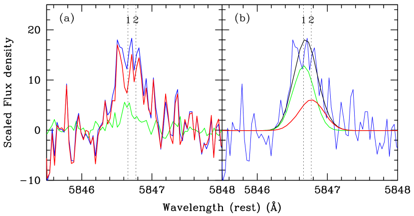
Figure 4.— (a) The observed line profile at $\lambda$5846.7 Å (blue line). The dotted lines are the rest wavelength of the He ii$\lambda$5846.7 and [Xe iii]$\lambda$5846.8 lines, which are indicated with the numbers 1 and 2, respectively. The line is composed of He ii$\lambda$5846.7 and [Xe iii]$\lambda$5846.8 transitions. The green line is the expected He ii$\lambda$5846.7 profile made by scaling intensity down and shifting wavelength of He ii$\lambda$6074.3 to He ii$\lambda$5846. The red line is the solo [Xe iii]$\lambda$5846.8 (method I). (b) The observed line profile at $\lambda$5846.7 Å (blue line). This line could be represented by two Gaussian components; the green line is He ii$\lambda$5846.7 and the red line is [Xe iii]$\lambda$5846.8. The black line is the sum of these two components (method II, See text in detail).

Table 6The Adopting electron temperatures and densities.

$T_{\epsilon}$ (K)	$n_{\epsilon}$ (cm-3)	Ions
9400	590	N0, O0
11 300	710	C+, N+, O+
11 300	1030	S+
13 280	2790	C2+, C3+, O2+, O3+, Ne+, Ne2+
		S2+, S3+, Cl2+, Ar2+, Ar3+, Xe2+

Table 7Ionic Abundances From CELs.

Xm+	$\lambda_{\rm lab}$	$I$($\lambda_{\rm lab}$)	Xm+/H+
C+	2326 Å	4.35(+2)$\pm$1.70(+1)	4.00(–4)$\pm$3.88(–5)
C2+	1906/9 Å	1.56(+3)$\pm$6.18(+2)	5.51(–4)$\pm$5.23(–5)
C3+	1549/51 Å	3.42(+2)$\pm$1.89(+1)	8.85(–5)$\pm$1.04(–5)
N0	5197.9 Å	5.10(–1)$\pm$1.33(–2)	8.88(–7)$\pm$1.77(–7)
	5200.3 Å	4.32(–1)$\pm$1.47(–2)	8.93(–7)$\pm$1.72(–7)
			8.91(–7)$\pm$1.75(–7)
N+	5754.6 Å	1.49(0)$\pm$4.30(–2)	1.17(–5)$\pm$8.85(–7)
	6548.0 Å	2.77(+1)$\pm$7.14(–1)	1.19(–5)$\pm$5.37(–7)
	6583.5 Å	8.07(+1)$\pm$2.02(0)	1.17(–5)$\pm$5.25(–7)
			1.18(–5)$\pm$5.33(–7)
O0	5577.3 Å	1.20(–1)$\pm$1.76(–2)	1.49(–5)$\pm$4.84(–6)
	6300.3 Å	6.40(0)$\pm$2.14(–1)	1.51(–5)$\pm$2.80(–6)
	6363.8 Å	2.11(0)$\pm$7.72(–2)	1.56(–5)$\pm$2.91(–6)
			1.52(–5)$\pm$2.86(–6)
O+	3726.0 Å	9.11(+1)$\pm$3.33(0)	4.55(–5)$\pm$3.14(–6)
	3728.8 Å	8.52(+1)$\pm$2.61(0)	4.58(–5)$\pm$3.12(–6)
	7320/30 Å	6.66(0)$\pm$2.11(–1)	4.98(–5)$\pm$4.39(–6)
	2470 Å	5.10(0)$\pm$1.82(0)	5.07(–5)$\pm$1.82(–5)
			4.58(–5)$\pm$3.16(–6)
O2+	1660/66 Å	5.43(+1)$\pm$2.03(+1)	2.91(–4)$\pm$1.12(–4)
	4361.2 Å	9.76(0)$\pm$2.31(–1)	9.66(–5)$\pm$7.63(–6)
	4931.8 Å	7.33(–2)$\pm$1.28(–2)	7.93(–5)$\pm$1.42(–5)
	4958.9 Å	2.24(+2)$\pm$3.10(0)	9.46(–5)$\pm$4.01(–6)
	5006.8 Å	6.67(+2)$\pm$2.62(+1)	9.76(–5)$\pm$5.50(–6)
			9.69(–5)$\pm$5.15(–6)
O3+	25.9 $\mu$m	3.09(+1)$\pm$2.84(0)	7.56(–6)$\pm$7.01(–7)
Ne+	12.8 $\mu$m	3.91(–1)$\pm$5.70(–2)	4.50(–7)$\pm$6.58(–8)
Ne2+	3868.8 Å	5.32(0)$\pm$2.25(–1)	2.26(–6)$\pm$1.43(–7)
	3967.5 Å	1.56(0)$\pm$5.90(–2)	1.59(–6)$\pm$9.58(–8)
	15.6 $\mu$m	3.56(0)$\pm$3.39(–1)	2.03(–6)$\pm$1.94(–7)
			2.08(–6) $\pm$ 1.53(–7)
S+	4068.6 Å	2.77(–1)$\pm$1.92(–2)	5.19(–8)$\pm$4.44(–9)
	6716.4 Å	5.05(–1)$\pm$2.76(–2)	2.23(–8)$\pm$1.46(–9)
	6730.8 Å	5.77(–1)$\pm$2.31(–2)	2.20(–8)$\pm$1.15(–9)
			2.21(–8)$\pm$1.29(–9)
S2+	6312.1 Å	1.06(–1)$\pm$1.29(–2)	8.15(–8)$\pm$1.07(–8)
	18.7 $\mu$m	9.15(–1)$\pm$1.00(–1)	8.17(–8)$\pm$9.01(–9)
			8.17(–8)$\pm$9.19(–9)
S3+	10.5 $\mu$m	1.77(0)$\pm$2.41(–1)	4.77(–8)$\pm$6.50(–9)
Cl2+	5517.7 Å	6.16(–2)$\pm$7.19(–3)	3.71(–9)$\pm$4.52(–10)
	5537.6 Å	6.16(–2) $\pm$ 6.60(–3)	3.60(–9) $\pm$ 4.05(–10)
			3.65(–9) $\pm$ 4.29(–10)
Ar2+	7135.8 Å	3.48(–1)$\pm$1.56(–2)	1.75(–8)$\pm$9.27(–10)
Ar3+	4711.4 Å	6.52(–2)$\pm$7.00(–3)	7.72(–9)$\pm$8.88(–10)
	4740.2 Å	5.94(–2)$\pm$4.35(–3)	7.56(–9)$\pm$6.33(–10)
			7.65(–9)$\pm$7.67(–10)
Xe2+	5846.7 Å	$>$2.59(–2)	$>$2.95(–10)a
Ba+	6141.7 Å	$<$9.83(–3)	$<$3.23(–11)b

We obtained 18 ionic abundances: C^+,2+,3+, N^0,1+, O^0,1+,2+,3+, Ne^+,2+, S^+,2+,3+, Ar^2+,3+, Cl²⁺, and Xe²⁺. The estimates of C^+,3+, O³⁺, Cl²⁺, and Xe²⁺ are reported for the first time. The ionic abundances were calculated by solving the statistical equilibrium equations for more than five levels in adopting $T_{\epsilon}$ and $n_{\epsilon}$. We used electron temperatures and densities for each ion that were determined using CEL plasma diagnostics. The adopted $T_{\epsilon}$ and $n_{\epsilon}$ values for each ion are listed in Table 6.

The derived ionic abundances are presented in Table 7. The last column contains the resulting ionic abundances, X^m+/H⁺, and their probable errors, which include errors from line intensities, electron temperature, and electron density. In the last line of each ion’s line series, we present the adopted ionic abundance and its error. These values are estimated from the weighted mean of the line intensity.

When calculating the C⁺ abundance, we subtracted contamination from [O iii] $\lambda$2321 Å to [C ii] $\lambda$2326 Å based on the theoretical intensity ratio of [O iii] $I$(2326 Å)/$I$(4363 Å) = 0.236. To determine the final S⁺ abundance, we excluded the values derived from the trans-aural line [S ii]$\lambda$4069 Å because this line would be contaminated from C iii $\lambda$4068 Å. For O²⁺, we excluded [O iii]$\lambda$1660/66 Å because of its large uncertainty.

Dinerstein et al. (2003) reported the upper limit intensities of [Ne ii]$\lambda$12.8 $\mu$m and [S iv]$\lambda$10.5 $\mu$m and estimated Ne⁺/H⁺$<$4.6(–6) and S³⁺/H⁺$<$3.8(–7) using the mid-IR spectra taken by TEXES/IRTF. The $Spitzer$ observations improved their estimates.

This is the first detection of [Xe iii]$\lambda$5846.8 Å (${}^{3}P_{2}{-}^{1}D_{2}$) in H4-1. The detection of this element is very rare because there are only a handful of detection cases in PNe (Sharpee et al., 2007; Sterling et al., 2009; García-Rojas et al., 2012; Otsuka et al., 2010).

The local continuum subtracted [Xe iii]$\lambda$5846.8 line profile is presented in Fig. 4. In high-excitation PNe such as H4-1, this line appears to be blended with He ii$\lambda$5846.7 ($n$=31-5; Pfund series). The blue line in Fig. 4(a) indicates the observed line profile. The $[$Fe ii$]$ $\lambda$5847.3 line possibly contributes to the emission line at $\lambda$5846, however, this line has poorer wavelength agreement and our photo-ionization model of H4-1 using CLOUDY code (Ferland et al., 1998) predicted that the intensity ratio of $I$([Fe ii]$\lambda$5846.7) to $I$(H$\beta$) is $<$1(–8). Therefore, the emission line at $\lambda$5846 would be a combination of the [Xe iii] and He ii lines.

We attempted to obtain the solo [Xe iii]$\lambda$5846.8 line flux by subtracting the contribution from He ii$\lambda$5846.7 using the following method (method I). First, we scaled the intensity of He ii$\lambda$6074.3 down to He ii$\lambda$5846.7 using the theoretical ratio of $I$($\lambda$5846.7)/$I$(6074.3), which is 0.271 in the case of $T_{\epsilon}$=11 970 K (=$T_{\epsilon}$(BJ)) and 1000 cm^-3 according to Storey & Hummer (1995). Second, we shifted the intensity peak wavelength of this scaled line to 5846.7 Å. The predicted He ii$\lambda$5846.7 is indicated by the green line in Fig. 4(a). Next, we subtracted this shifted line from the 5846 Å line. Finally, we obtained an intensity of the [Xe iii] $\lambda$5846.8 line of 3.63(–2)$\pm$1.04(–2), as indicated by the red line in Fig. 4(a).

We also attempted to obtain the [Xe iii]$\lambda$5846.8 using Gaussian fitting, as shown in Fig. 4(b) (method II). As constraints, we fix the rest wavelengths of the intensity peak and FWHM velocities to equal 5846.7 Å and 18.33 km s^-1 for He ii$\lambda$5846.7, respectively, and 5846.8 and 21.90 km s^-1 for [Xe iii]$\lambda$5846.8. Here, 18.33 km s^-1 and 21.90 km s^-1 correspond to the FWHM velocities of He ii$\lambda$6074.3 and [Cl iii]$\lambda$5537 (I.P.=23.81 eV). Because the I.P. of Xe²⁺ (21.21 eV) is very close to Cl²⁺, we assumed that the FWHM velocity of $[$Xe iii$]$ is almost identical to that of [Cl iii]$\lambda$5537. In method II, we obtained $I$($[$Xe iii$]$$\lambda$5846.8)$>$1.42(–2).

Based on the above analyses, it is probable that [Xe iii] $\lambda$5846.8 would be in the HDS spectrum. However, we need to carefully consider the estimation of the $[$Xe iii$]$$\lambda$5846.8 line intensity; because we could not detect any Pfund series He ii lines with an upper $n$ from 29 to 21 and $>$32, He ii$\lambda$5846.7 may be not in the HDS spectrum or it may be present at a very low intensity. The emission line at 5846.8 Å would be mostly from the [Xe iii] $\lambda$5846.8 line. In this work, we determined the lower limit Xe²⁺ and Xe abundances using method I based on the transition probabilities of Biemont et al. (1995) and the collisional impacts of Schoening & Butler (1998).

We could not retrieve strong lines for Ba ii $\lambda$4934.6 Å and 6141.7 Å from the HDS spectrum because both lines were deeply affected by moonlight. Therefore, we calculated an upper limit for the expected Ba⁺ abundance of 3.23(–10) using the 1-$\sigma$ flux density at Ba ii$\lambda$6141.7 ($I$(6141.7 Å)/$I$(H$\beta$)=9.83(–3), $I$(H$\beta$)=100) with $T_{\epsilon}$=11 300 K, $n_{\epsilon}$=1030 cm^-3, and FWHM velocity = 19 km s^-1. In the Ba⁺ calculation, we used transition probabilities from Klose et al. (2002) and collisional impacts from Schoening & Butler (1998)

3.4. RL Ionic Abundances

Table 8Ionic Abundances From RLs.

Xm+	Multi.	$\lambda_{\rm lab}$	$I$($\lambda_{\rm lab}$)	Xm+/H+
He+	V11	5875.62 Å	1.49(+1)$\pm$3.63(–1)	1.00(–1)$\pm$4.09(–2)
	V14	4471.47 Å	4.49(0)$\pm$9.31(–2)	8.46(–2)$\pm$3.20(–2)
	V46	6678.15 Å	3.40(0)$\pm$9.01(–2)	7.97(–2)$\pm$3.27(–2)
	V48	4921.93 Å	1.01(0)$\pm$1.70(–2)	7.52(–2)$\pm$3.34(–2)
	V51	4387.93 Å	5.32(–2)$\pm$1.64(–2)	8.68(–2)$\pm$3.86(–2)
				9.30(–2)$\pm$3.77(–2)
He2+	3.4	4685.68 Å	1.83(+1)$\pm$2.27(–1)	1.54(–2)$\pm$2.04(–3)
C2+	V4	3920.68 Å	4.97(–2)$\pm$1.84(–2)	1.17(–3)$\pm$4.94(–4)
	V6	4267.15 Å	1.12(0)$\pm$3.50(–2)	1.15(–3)$\pm$1.80(–4)
	V16.04	6151.27 Å	5.93(–2)$\pm$9.11(–3)	1.36(–3)$\pm$2.79(–4)
	V17.04	6461.71 Å	1.34(–1)$\pm$1.07(–2)	1.33(–3)$\pm$2.59(–4)
	V17.06	5342.19 Å	7.85(–2)$\pm$7.72(–3)	1.49(–3)$\pm$2.99(–4)
	V17.06	5342.43 Å	8.23(–2)$\pm$1.43(–2)	1.56(–3)$\pm$3.85(–4)
				1.21(–3)$\pm$2.19(–4)
C2+	V1	4647.42 Å	2.32(–1)$\pm$7.15(–3)	3.64(–4)$\pm$4.37(–5)
	V1	4650.25 Å	1.47(–1)$\pm$5.89(–3)	3.86(–4)$\pm$4.74(–5)
	V16	4067.87 Å	1.62(–1)$\pm$1.51(–2)	4.25(–4)$\pm$7.22(–5)
	V16	4070.14 Å	2.61(–1)$\pm$1.76(–2)	3.82(–4)$\pm$6.00(–5)
				3.86(–4)$\pm$5.55(–5)
C3+	V1	4658.20 Å	6.48(–2)$\pm$4.19(–3)	1.55(–5)$\pm$2.45(–6)
N3+	V2	4634.12 Å	8.27(–2)$\pm$1.11(–2)	6.51(–5)$\pm$1.22(–5)
	V2	4640.64 Å	1.48(–1)$\pm$5.84(–3)	6.50(–5)$\pm$8.88(–6)
				6.50(–5)$\pm$1.01(–5)
O2+	V1	4638.86 Å	5.71(–2)$\pm$5.99(–3)	3.51(–4)$\pm$5.74(–5)
	V1	4641.81 Å	4.72(–2)$\pm$4.90(–3)	1.81(–4)$\pm$2.32(–5)
	V1	4651.33 Å	2.36(–2)$\pm$5.42(–3)	1.40(–4)$\pm$3.66(–5)
	V1	4661.63 Å	3.53(–2)$\pm$5.14(–3)	1.96(–4)$\pm$3.77(–5)
	V2	4349.43 Å	2.80(–2)$\pm$5.97(–3)	1.41(–4)$\pm$3.49(–5)
				1.69(–4)$\pm$3.40(–5)
O3+	V2	3754.70 Å	1.82(–1)$\pm$1.97(–2)	3.47(–4)$\pm$5.80(–5)
	V2	3757.24 Å	7.79(–2)$\pm$1.27(–2)	3.35(–4)$\pm$6.92(–5)
				3.43(–4)$\pm$6.13(–5)

The estimated RL ionic abundances are listed in Table 8. The calculations of C^3+,4+, N³⁺, and O^2+,3+ abundances were performed for the first time. The Case B assumption applies to lines from levels that have the same spin as the ground state, and the Case A assumption applies to lines of other multiplicities. In the last line of each ion’s line series, we present the adopted ionic abundance and the error estimate from the line intensity-weighted mean. Because the RL ionic abundances are insensitive to the electron density under $\lesssim$10⁸ cm^-3, we adopted $n_{\epsilon}$=10⁴ cm^-3 for He²⁺, C^2+,3+,4+, N³⁺, and O^2+,3+ and $n_{\epsilon}$=10² cm^-3 for He⁺. The emission coefficients are the same as those used in Otsuka et al. (2010).

We detected multiplet V2 N iii lines, however, these lines are not recombination lines, but resonance lines. Because we detected the O iii resonance line, the intensity of the resonance line N iii $\lambda$374.36 Å (2$p$ ${}^{2}P^{0}$-3$d$ ${}^{2}D$) is enhanced by O iii resonance lines at the wavelength of 374.11 Å (2$p^{2}$ ${}^{3}P$-3$s^{3}$ $P^{0}$). The line intensities of the multiplet V2 lines can be enhanced by O iii lines. Furthermore, the detected V2 O iii lines might be excited by the Bowen fluorescence mechanism or by the charge exchange of O³⁺ and H⁰ instead of by recombination. Therefore, we did not use the N³⁺ and O³⁺ abundances to determine elemental RL N and O abundances.

We detected the multiplet V1 and V2 O ii lines. Ruiz et al. (2003), Peimbert et al. (2005), and García-Rojas et al. (2009) pointed out that the upper levels of the transitions in the V1 O ii line are not in local thermal equilibrium (LTE) for $n_{\epsilon}$$<$ 10 000 cm^-3, and that the abundances derived from each individual line could differ by a factor of $\sim$4 (García-Rojas et al., 2009). However, the V2 lines are not affected by non-LTE effects. Because H4-1 is a low-density PN ($<$3000 cm^-3), we performed the non-LTE corrections using equations (8) through (10) from Peimbert et al. (2005) with $n_{\epsilon}$=2000 cm^-3. The resulting O²⁺ abundances determined using the V1 and V2 lines are in good agreement, except for the O ii $\lambda$4638.86 line. This line was therefore excluded in the final determination of the RL O²⁺ abundance.

3.5. Elemental Abundances

Table 9Adopted ionization correction factors (ICFs).

X	Line	ICF(X)	X/H
He	RL	1	He++He2+
C	CEL	$\rm\frac{1}{1-\left(\frac{C^{4+}}{C}\right)_{RL}}$	ICF(C)(C++C2++C3+)
	RL	$\rm\frac{1}{1-\left(\frac{N^{+}}{N}\right)_{CEL}}$	ICF(C)(C2++C3++C4+)
N	CEL	$\rm\left(\frac{O}{O^{+}}\right)_{CEL}$	ICF(N)N+
O	CEL	1	O++O2++O3+
	RL	$\rm\left(\frac{O}{O^{2+}}\right)_{CEL}$	ICF(O)O2+
Ne	CEL	$\rm\left(\frac{O}{O^{+}+O^{2+}}\right)_{CEL}$	ICF(Ne)(Ne++Ne2+)
S	CEL	1	$\rm S^{+}+S^{2+}+S^{3+}$
Cl	CEL	$\rm{\left(\frac{Ar}{Ar^{2+}}\right)}$	ICF(Cl)Cl2+
Ar	CEL	$\rm\frac{1}{1-\left(\frac{N^{+}}{N}\right)_{CEL}}$	ICF(Ar)$\rm\left(Ar^{2+}+Ar^{3+}\right)$
Xe	CEL	$\rm{\left(\frac{Ar}{Ar^{2+}}\right)}$	ICF(Xe)Xe2+
Ba	CEL	1	ICF(Ba)Ba+

Table 10The Elemental Abundances From CEL and RLs.

X	Types of	X/H	log(X/H)+12	[X/H]	log(X⊙/H)+12	ICF(X)
	Emissions
He	RL	1.08(–2)$\pm$3.78(–2)	11.04$\pm$0.15	+0.11$\pm$0.15	10.93$\pm$0.01	1.00
C	RL	2.33(–3)$\pm$6.91(–4)	9.37$\pm$0.13	+0.98$\pm$0.13	8.39$\pm$0.04	1.44$\pm$0.38
C	CEL	1.04(–3)$\pm$4.42(–4)	9.02$\pm$0.18	+0.63$\pm$0.19	8.39$\pm$0.04	1.01$\pm$0.42
N	CEL	3.85(–5)$\pm$3.56(–6)	7.59$\pm$0.04	–0.24$\pm$0.06	7.83$\pm$0.05	3.28$\pm$0.26
O	RL	2.63(–4)$\pm$7.54(–5)	8.42$\pm$0.12	–0.27$\pm$0.13	8.69$\pm$0.05	1.55$\pm$0.32
O	CEL	1.50(–4)$\pm$6.09(–6)	8.18$\pm$0.02	–0.51$\pm$0.05	8.69$\pm$0.05	1.00
Ne	CEL	2.67(–6)$\pm$5.87(–7)	6.43$\pm$0.10	–1.44$\pm$0.14	7.87$\pm$0.10	1.05$\pm$0.22
S	CEL	1.36(–7)$\pm$1.01(–8)	5.13$\pm$0.03	–2.06$\pm$0.05	7.19$\pm$0.04	1.00
Cl	CEL	7.57(–9)$\pm$2.24(–9)	3.88$\pm$0.13	–1.62$\pm$0.33	5.50$\pm$0.30	2.07$\pm$0.56
Ar	CEL	3.63(–8)$\pm$9.65(–9)	4.56$\pm$0.12	–1.99$\pm$0.14	6.55$\pm$0.08	1.45$\pm$0.38
Xe	CEL	$>$5.05(–10)	$>$2.75	$>$+0.48	2.27$\pm$0.02	1.94$\pm$0.51
Ba	CEL	$<$3.23(–10)	$<$2.51	$<$+0.33	2.18$\pm$0.03	1

Table 11Elemental Abundances derived by previous works and by this work.

References	He	C	N	O	Ne	S	Cl	Ar	Xe	Ba
This work (RL)	11.04	9.37	$\cdots$	8.42	$\cdots$	$\cdots$	$\cdots$	$\cdots$	$\cdots$	$\cdots$
This work (CEL)	$\cdots$	9.02	7.56	8.18	6.43	5.13	3.88	4.56	$>$2.75	$<$2.51
Kwitter et al. (2003)	11.08	$\cdots$	7.76	8.30	6.60	5.30	$\cdots$	4.30	$\cdots$	$\cdots$
Henry et al. (1996)a	11.00	8.68	7.76	8.40	6.44	$\cdots$	$\cdots$	$\cdots$	$\cdots$	$\cdots$
Torres-Peimbert & Peimbert (1979, $t^{2}$=0)	10.99	9.39b	7.75	8.37	6.68	$\cdots$	$\cdots$	$\cdots$	$\cdots$	$\cdots$
Torres-Peimbert & Peimbert (1979, $t^{2}$=0.035)	10.99	9.39b	7.87	8.50	6.80	$\cdots$	$\cdots$	$\cdots$	$\cdots$	$\cdots$

Note. — The CEL abundances with $t^{2}\neq$ 0 by us are listed in Table 13.

Table 12C, Ar, Xe, and Ba abundances in PNe.

Nebulae	$[$C/Ar$]$	$[$Xe/Ar$]$	$[$Ba/Ar$]$	$[$Ba/Xe$]$	$[$Ar/H$]$	Ref.
IC418	+0.94	+0.94	+0.33	–0.61	–0.54	(1),(2)
IC2501	+0.66	–0.03	–0.06	+0.09	–0.27	(1),(3),(4)
IC4191	+0.93	+0.50	+0.83	+0.33	–0.51	(1),(5),(6)
M3-15	+0.23	+1.15	$\cdots$	$\cdots$	–0.25	(7),(8)
NGC2440	+0.71	–0.36	+0.79	+1.15	–0.24	(1),(9)
NGC5189	–0.10	–0.08	$\cdots$	$\cdots$	–0.06	(7),(8)
NGC7027	+0.91	+0.93	+0.43	–0.50	–0.20	(1),(10)
PC14	+0.43	+0.13	$\cdots$	$\cdots$	–0.17	(7),(8)
Pe1-1	+0.74	+1.00	$\cdots$	$\cdots$	–0.23	(7),(8)
BoBn1	+2.85	$<$+1.95	$>$+2.34	$>$+0.38	–2.22	(11)
H4-1	+2.62	$>$+2.47	$<$+2.32	$<$–0.18	–1.99	(7)

Note. — The abundances are estimated from CELs, except for C in IC4191 which is estimated using recombination lines.

References. — (1) Sharpee et al. (2007); (2) Pottasch et al. (2004); (3) Henry et al. (2004); (4) Rola & Stasińska (1994); (5) Pottasch et al. (2005); (6) Tsamis et al. (2004); (7) This work; (8) García-Rojas et al. (2012); (9) Bernard Salas et al. (2002); (10) Zhang et al. (2005b); (11) Otsuka et al. (2010)

The elemental abundances were estimated using an ionization correction factor, ICF(X), which is based on the ionization potential. The ICF(X) for each element is listed in Table 9.

The He abundance is the sum of the He⁺ and He²⁺ abundances. We assume that the C abundance is the sum of the C⁺, C²⁺, C³⁺, and C⁴⁺ abundances, and we corrected for the CEL C⁴⁺ and the RL C⁺. The N abundance is the sum of N⁺, N²⁺, and N³⁺, and we corrected for the N²⁺ and N³⁺ abundances. The O abundance is the sum of the O⁺, O²⁺, and O³⁺ abundances. For the RL O abundance, we estimated the O⁺ and O³⁺ abundances. The Ne abundance is the sum of the Ne⁺, Ne²⁺, and Ne³⁺ abundances, and we corrected for the Ne³⁺ abundance. The S abundance is the sum of the S⁺, S²⁺, and S³⁺ abundances. The Cl abundance is the sum of the Cl⁺, Cl²⁺, Cl³⁺, and Cl⁴⁺ abundances, correcting for Cl⁺, Cl³⁺, and Cl³⁺. The Ar abundance is the sum of the Ar⁺, Ar²⁺, Ar³⁺, and Ar⁴⁺ abundances, correcting for the Ar⁺ and Ar⁴⁺ abundances. The Xe abundance is the sum of the Xe⁺, Xe²⁺, Xe³⁺, and Xe⁴⁺ abundances, correcting for the Xe⁺, Xe³⁺, and Xe⁴⁺ abundances. We did not correct for the ionization of Ba.

The resulting elemental abundances are listed in Table 10. The types of emission lines used for the abundance estimations are specified in the second column. The number densities of each element relative to hydrogen are listed in the third column. The fourth column lists the number densities and the fifth column lists the number densities relative to the solar value. The last two columns are the solar abundances and the adopted ICF values. We referred to Asplund et al. (2009) for N and Cl, and Lodders (2003) for the other elements.

The [C/O] abundances are +1.25$\pm$0.19 dex from the RL and +1.14$\pm$0.20 dex from the CEL, therefore H4-1 is an extremely C-enhanced PN. However, as shown in the fifth column of Table 10, the C and O abundances are slightly different between RLs and CELs. The C and O abundance discrepancies could be explained by small temperature fluctuations in the nebula. We discuss the C and O abundance discrepancies in the next section.

In Table 11, we compiled results for H4-1. We improved the C, O, Ne, S, Ar abundances and newly added the Cl and Xe abundances, thanks to high-dispersion Subaru/HDS spectra and the detection of many different ionization stage ions. The large discrepancy in C abundance between the RL (Torres-Peimbert & Peimbert, 1979) and the CEL (Henry et al., 1996) is reduced as a result of our work.

In Table 3.5, we summarize the Xe abundances in 11 Galactic PNe. Using the line lists from García-Rojas et al. (2012), we estimated the Xe abundances of M3-15, NGC5189, PC14, and Pe1-1 in $T_{\epsilon}$([O iii]) and $n_{\epsilon}$([Cl iii]). For the above PNe, we removed the contribution of He ii$\lambda$5846.7 to [Xe iii]$\lambda$5846.8 using method I as described in Section 3.3. The Xe abundance in H4-1 is the highest among these PNe. In the next section, we also discuss how much Xe in H4-1 is a product of AGB nucleosynthesis in the progenitor.

4. Discussion

4.1. C and O abundance discrepancies

Table 13The Ionic and Elemental Abundances From CELs in $t^{2}$=0.03.

Xm+	(Xm+/H+)${}_{t^{2}\neq 0}$	Xm+	(Xm+/H+)${}_{t^{2}\neq 0}$
C+	3.98(–4)$\pm$5.06(–5)	Ne2+	2.42(–6)$\pm$1.91(–7)
C2+	6.25(–4)$\pm$9.38(–5)	S+	2.27(–8)$\pm$1.37(–9)
C3+	8.96(–5)$\pm$1.85(–5)	S2+	8.63(–8)$\pm$9.79(–9)
N+	1.21(–5)$\pm$5.77(–7)	S3+	3.48(–8)$\pm$4.09(–9)
O+	4.83(–5)$\pm$3.78(–6)	Cl2+	4.37(–9)$\pm$5.21(–10)
O2+	1.17(–4)$\pm$6.82(–6)	Ar2+	2.05(–8)$\pm$1.12(–9)
O3+	7.80(–6)$\pm$7.23(–7)	Ar3+	9.25(–9)$\pm$9.58(–10)
Ne+	4.66(–7)$\pm$6.81(–8)	Xe2+	$>$3.61(–10)
X	$\log$(X/H)${}_{t^{2}\neq 0}$+12	X	$\log$(X/H)${}_{t^{2}\neq 0}$+12
C	9.05$\pm$0.18	S	5.15$\pm$0.03
N	7.64$\pm$0.04	Cl	3.95$\pm$0.13
O	8.24$\pm$0.02	Ar	4.62$\pm$0.11
Ne	6.48$\pm$0.10	Xe	$>$2.84

Note. — The RL elemental C and O abundances in $t^{2}$=0.03 are 9.35$\pm$0.13 and 8.40$\pm$0.12, respectively (See text in detail).

The RL to CEL abundance ratio, also known as the abundance discrepancy factor (ADF), in C²⁺, C³⁺, and O²⁺ is 2.20$\pm$0.45, 4.36$\pm$0.81, and 1.75$\pm$0.36, respectively. For most PNe, ADFs are typically between 1.6 and 3.2 (see Liu, 2006).

The value of $T_{\epsilon}$(He i) is comparable to the value of $T_{\epsilon}$(BJ) within estimation error. According to Zhang et al. (2005a), if $T_{\epsilon}$(He i) is lower than $T_{\epsilon}$(BJ), then the chemical abundances in the nebulae have two different abundance patterns. Otherwise, the abundance discrepancy between the CELs and the RLs is caused by temperature fluctuations within the nebula.

We attempted to explain the discrepancies in C and O abundance by including temperature fluctuations in the nebula. Peimbert et al. (1993) extended this effect to account for RL and CEL O²⁺ abundance discrepancies by introducing the mean electron temperature $T_{0}$ and the electron temperature fluctuation parameter $t^{2}$, as follows,

$$T_{0}({\rm X}^{i+})=\frac{\int T_{\epsilon}n_{\epsilon}N({\rm X}^{i+})~{}dV}{\int n_{\epsilon}N({\rm X}^{i+})~{}dV},$$ (2)

$$t^{2}=\frac{\int(T_{\epsilon}-T_{0})^{2}n_{\epsilon}N({\rm X}^{i+})~{}dV}{T_{0}\int n_{\epsilon}N({\rm X}^{i+})~{}dV}.$$ (3)

Using this temperature fluctuation model, we attempted to explain the discrepancy in C^2+,3+ and O²⁺ abundance.

Following the methods of Peimbert & Torres-Peimbert (1971) and Peimbert (2003), we estimated the mean electron temperatures and $t^{2}$. When $t^{2}$ $\ll$ 1, the observed $T_{\epsilon}$([O iii]), $T_{\epsilon}$([N ii]), and $T_{\epsilon}$(BJ) are written as follows,

$$T_{\epsilon}({\rm[O\,{\sc III}]})=T_{0,h}\left[1+\frac{1}{2}\left(\frac{91\,300}{T_{0,h}}-3\right)t_{h}^{2}\right],$$ (4)

$$T_{\epsilon}({\rm[N\,{\sc II}]})=T_{0,l}\left[1+\frac{1}{2}\left(\frac{69\,070}{T_{0,l}}-3\right)t_{l}^{2}\right],$$ (5)

$$T_{\epsilon}({\rm BJ})=T_{0}\left(1-1.67~{}t^{2}\right),$$ (6)

where $T_{0,h}$ & $t_{h}^{2}$ and $T_{0,h}$ & $t_{l}^{2}$ are the average temperatures and temperature fluctuation parameters in high- and low-ionization zones, respectively; C⁺, N⁺, O⁺, and S⁺ are in low-ionization zones and the other elements are in high-ionization zones (See Table 9).

Based on the assumption that $t^{2}$=$t_{h}^{2}$=$t_{l}^{2}$, we found that $T_{0,h}$=12 590$\pm$340 K, $T_{0,l}$=10 760$\pm$290 K, $T_{0}$=12 590$\pm$1100 K, and $t^{2}$=0.030$\pm$0.007 minimize the ADFs in C^2+,3+ and O²⁺ using the combination of equations (4)-(6). Our determined $t^{2}$ is in agreement with Torres-Peimbert & Peimbert (1979), who determined $t^{2}$=0.035.

Next, the average line-emitting temperatures for each line at $\lambda$, $T_{\epsilon}(\lambda)$, and $T_{\epsilon}$(H$\beta$) can be written by following the method of Peimbert et al. (2004):

$$T_{\epsilon}(\lambda)=T_{0,h,l}$$

$$\times\left\{1+\left[\frac{(\Delta{E}/kT_{0,h,l})^{2}-3(\Delta{E}/kT_{0,h,l})+0.75}{(\Delta{E}/kT_{0,h,l})-0.5}\right]\frac{t^{2}}{2}\right\},$$ (7)

$$T_{\epsilon}({\rm H\beta})=T_{0,h,l}\left(1-\frac{1.633}{2}t^{2}\right),$$ (8)

where $T_{0,h,l}$ is 12 590$\pm$340 K for the elements in high ionization zone and is 10 760$\pm$290 K for those in low ionization zone, the $\Delta{E}$ is the difference energy between the upper and lower level of of the target lines, $k$ is Boltzmann constant, respectively. Finally, the ionic abundances can be estimated by following the method of Peimbert et al. (2004), which accounts for the effects of fluctuations in temperature:

$$\frac{N({\rm X}^{m+})_{t^{2}\neq 0.00}}{N({\rm X}^{m+})_{t^{2}=0.00}}=\frac{T_{\epsilon}({\rm H\beta})^{-0.87}T_{\epsilon}(\lambda)^{0.5}}{T_{\epsilon}([\rm O\,{\sc III}],[N\,{\sc II}])^{-0.37}}$$

$$\times\exp\left[\frac{\Delta E}{kT_{\epsilon}(\lambda)}-\frac{\Delta E}{kT_{\epsilon}([\rm O\,{\sc III}],[N\,{\sc II}])}\right].$$ (9)

The resulting CEL ionic and elemental abundances are summarized in Table 13. The ADFs are slightly improved for C²⁺ and O²⁺, with values of 1.94$\pm$0.45 and 1.45$\pm$0.30, respectively, whereas the ADF for C³⁺ remains high, with a value of 4.31$\pm$1.03. Because most of the ionic C abundances are in a doubly ionized stage, and the CEL C²⁺ abundance approaches that of the RL C²⁺, the elemental CEL C abundance is very close to the RL C abundance (9.35 dex for the RL and 9.05 dex for the CEL), resolving the C abundance discrepancy. The elemental O abundances agree within error, 8.40 for the RL and 8.24 for the CEL.

Two difference abundance patterns could cause the ionic C^2+,3+ and O²⁺ abundances. However, even if these abundance patterns appear in H4-1, the difference between these ionic abundances would be negligible.

4.2. Comparison with theoretical model

Table 14 Comparison of the observed abundances with the model prediction.

References	C	N	O	Ne	S	Ar	Xe	Ba
0.9 $M_{\odot}$	9.04	7.57	7.63	7.87	5.00	4.28	1.56	2.37
initial abundances	6.28	5.68	6.54	5.78	4.97	4.25	0.01	0.00
2.0 $M_{\odot}$	9.55	6.84	7.93	8.66	5.34	4.57	2.11	2.52
+ $r$+2.0 dex
initial abundances	6.06	4.64	6.82	6.06	5.26	4.49	1.90	1.29
This work ($t^{2}$=0)	9.02	7.56	8.18	6.43	5.13	4.56	$>$2.75	$<$2.51

The large enhancement of the Xe abundance is the most remarkable finding for H4-1. In this section, we compare the observed abundances with the nucleosynthesis models for the initially 0.9 $M_{\odot}$ and 2.0 $M_{\odot}$ single stars with [X/H]=–2.19 from Lugaro et al. (2012), and we verify whether the observed Xe abundance could be explained using their models. From the galaxy chemical evolution model of Kobayashi et al. (2011), an [Fe/H] ratio of about –2.30 in H4-1 is estimated using the relation [Fe/H]=[Ar/H]-0.30. Therefore, the results of Lugaro et al. (2012) are good comparisons.

For the initially 0.9 $M_{\odot}$ star model, Lugaro et al. (2012) adopted scaled-solar abundances as the initial composition for all elements from C to Pb. Both the initial Xe and Ba abundances are $\sim$0, meaning that the final predicted abundances of these two elements are pure products of the $s$-process in their progenitors. In the 2.0 $M_{\odot}$ model, they initially adopted the [$r$/Fe]=+2. In Table 14, we compare our results with the predictions by Lugaro et al. (2012). The initial abundances are also listed. The models of Lugaro et al. (2012) include a partial mixing zone (PMZ) of 2(–3) $M_{\odot}$ that produces a ¹³C pocket during the interpulse period and releases extra free neutrons ($n$) through ¹³C($\alpha$,n)¹⁶O to obtain $n$-process elements. The 0.9 $M_{\odot}$ and the 2.0 $M_{\odot}$ star models predict that the respective stars experienced 38 and 27 times thermal pulses and the occurrence of a TDU.

The 0.9 $M_{\odot}$ model gives a good agreement with the observed C and N abundances, however, there are discrepancies between the observed and the model predicted $\alpha$-elements. The production of Xe is mainly a result of the $r$-process; Bisterzo et al. (2011) reported that the solar Xe and Eu are mainly from the $r$-process (84.6 $\%$ and 94 $\%$, respectively), although the contribution from the $r$-process to the Xe is disputable. The 0.9 $M_{\odot}$ model predicted the Xe/H abundance of 3.63(–11), while the observed abundance in H4-1 is 5.62(–10). Therefore, most the xenon in H4-1 is produced by the $r$-process in primordial SNe.

If the progenitor of H4-1 was formed in an $r$-process rich environment, the observed $\alpha$ elements and Xe could be explained. Compared to the 0.9 $M_{\odot}$ model, except for N and Ne, the $r$-process enhanced model for 2.0 $M_{\odot}$ stars explains the observed O, S, Ar, and Xe abundances well. About 0.2-0.3 dex of the observed $\alpha$-elements are SN products.

Through comparison with the theoretical models, we suppose that the observed Xe is mostly synthesized by $r$-process in SNe. The observed abundances could be explained by the model for 2.0 $M_{\odot}$ stars with the initial [$r$/Fe]=+2.0.

4.3. Comparison with CEMP stars and the evolution and evolution of H4-1

Figure 5.— The [Ba/(Eu or Xe)] versus [C/O] diagram. For H4-1, we used the [Ba/Xe] abundance. The [Ba/Xe] abundance of H4-1 is the upper limit. We used the abundances of CEMP stars provided by Suda et al. (2011). CEMP stars are classified as the criteria summarized in Table 15. The [Fe/H] of CEMP stars plotted in this diagram is from –4.75 to -2.03 in CEMP-$no$, from –2.7 to –2.2 in CEMP-$s$, and from –2.72 to –2.03 in CEMP-$r$/$s$, respectively.

Table 15Classification of CEMP stars in this work.

Class	Criteria
CEMP-$s$	[Fe/H]$\leq$–2,[C/Fe]$>$+1.0,[Ba/Fe]$>$+1.0,[Ba/Eu]$>$+0.5
CEMP-$r$/$s$	[Fe/H]$\leq$–2,[C/Fe]$>$+1.0,[Ba/Fe]$>$+1,0$<$[Ba/Eu]$<$+0.5
CEMP-$no$	[Fe/H]$\leq$–2,[C/Fe]$>$+1.0,[Ba/Fe]$<$0.0

Note. — In H4-1, the expected [Fe/H] and [Ba/Fe] are –2.3 and $<$+2.6 and the observed [C/Fe] and [Ba/Xe] are +2.83 and $<$–0.15, respectively.

Although the models by Lugaro et al. (2012) explain the observed abundances, it is difficult to explain the evolutional time scale of H4-1 with a 2.0 $M_{\odot}$ single-star evolution models, because such mass stars cannot survive in the Galactic halo up to now.

Therefore, it is possible that H4-1 evolved from a binary, similar to the evolution of CEMP stars, and its progenitor was polluted by SNe. Our definition of CEMP stars is summarized in Table 15, following Beers & Christlieb (2005). CEMP-$s$ stars are $s$-process rich, CEMP-$r$/$s$ are both $s$- and $r$-process rich. The CEMP stars which are neither CEMP-$s$ nor CEMP-$r$/$s$ are classified as the CEMP-$no$. Since the expected [Fe/H] and [Ba/Fe] are –2.3 and $<$+2.6 and the observed [C/Fe] and [Ba/Xe] are +2.83 and $<$–0.15, respectively, H4-1 can be classified as CEMP-$r$/$s$ or CEMP-$no$.

In Fig. 5, we present the [Ba/(Eu or Xe)] versus [C/O] diagram between H4-1 and CEMP stars. The data of CEMP stars are taken from Suda et al. (2011) and the classification is based on Table 15. The metallicities of CEMP-$s$ and CEMP-$r$/$s$ stars are widely spread, while those of CEMP-$no$ are mostly $\lesssim$–3 (e.g., Aoki et al., 2007). Fig. 5 indicates that H4-1 is similar to CEMP-$r$/$s$ and CEMP-$no$, assuming that the [Eu/H] abundance in H4-1 is similar to its [Xe/H] abundance.

Although H4-1 has a similar origin and evolution as CEMP-$r/s$ and CEMP-$no$ stars, the origin of these CEMP stars is a topic of much debate (Lugaro et al., 2012; Bisterzo et al., 2011; Jonsell et al., 2006; Ito et al., 2013; Zijlstra, 2004). As proposed by Zijlstra (2004) to explain the abundances of $r/s$-rich stars, the progenitor of H4-1 might be a binary composing of e.g, $\sim$0.8-0.9 $M_{\odot}$ and $\sim$5 $M_{\odot}$ (from their Fig. 2), which might evolve into a SN. However, there are problems on the N and Xe productions in such massive primary scenario for explanation of H4-1’s evolution. For instance, the 5 $M_{\odot}$ with $r$+0.4 dex models by Lugaro et al. (2012) predicted highly enhanced N (9.11) by the hot bottom burning and low Xe abundances (0.99 dex). While, Suda et al. (2013) argued that the inclusion of mass-loss suppression in metal-poor AGB stars can inhibit such N-enhanced metal-poor stars. Therefore, at the present, we think that the primary star should have never experienced the hot bottom burning.

If bipolar nebulae are created by stable mass-transfer during Roche lobe overflow, the initial mass ratio of the primary to secondary is $\sim$1-2, according to Phillips (2000). If this is the case for the bipolar nebula formation in H4-1 and the secondary is $\sim$0.8-0.9 $M_{\odot}$, the primary star would be $\sim$0.8-1.8 $M_{\odot}$. For example, Otsuka et al. (2010) explain the observed chemical abundances of BoBn1 using the binary model composed of 0.75 $M_{\odot}$ + 1.5 $M_{\odot}$ stars.

5. Summary

We analyzed the multi-wavelength spectra of the halo PN H4-1 from Subaru/HDS, GALEX, SDSS, and Spitzer/IRS in order to to determine chemical abundances, in particular, $n$-capture elements, solve the C abundance discrepancy problem, and obtain insights on the origin and evolution of H4-1. We determined the abundances of 10 elements based on the over 160 lines detected in those data. The C and O abundances were derived from both CELs and RLs. We found the discrepancies between the CEL and the RL abundances of C and O, respectively and they can be explained by considering temperature fluctuation effect. The large discrepancy in the C abundance between CEL and RL in H4-1 was solved by our study. In HDS spectrum, we detected the [Xe iii]$\lambda$5846 Å line in H4-1 for the first time. H4-1 is the most Xe enhanced PN among the Xe detected PNe. The observed abundances can be explained by a $\sim$2.0 $M_{\odot}$ single star model with initially [$r$/Fe]=+2.0 of Lugaro et al. (2012). The observed Xe abundance would be a product of the $r$-process in primordial SNe. About 0.2-0.3 dex of the $\alpha$ elements are also the products by these SNe. The [C/O]-[Ba/(Eu or Xe)] diagram suggests that the progenitor of H4-1 shares the evolution with CEMP-$r$/$s$ and CEMP-$no$ stars. The progenitor of H4-1 is a presumably binary formed in an $r$-process rich environment.

References

- Aoki et al. (2007) Aoki W., Beers T.C., Christlieb N., et al., 2007, ApJ 655, 492
- Asplund et al. (2009) Asplund M., Grevesse N., Sauval A.J., Scott P., 2009, ARA&A 47, 481
- Beers & Christlieb (2005) Beers T.C., Christlieb N., 2005, ARA&A 43, 531
- Benjamin et al. (1999) Benjamin R.A., Skillman E.D., Smits D.P., 1999, ApJ 514, 307
- Bernard Salas et al. (2002) Bernard Salas J., Pottasch S.R., Feibelman W.A., Wesselius P.R., 2002, A&A 387, 301
- Biemont et al. (1995) Biemont E., Hansen J.E., Quinet P., Zeippen C.J., 1995, A&AS 111, 333
- Bisterzo et al. (2011) Bisterzo S., Gallino R., Straniero O., Cristallo S., Käppeler F., 2011, MNRAS 418, 284
- Boothroyd & Sackmann (1988) Boothroyd A.I., Sackmann I.J., 1988, ApJ 328, 671
- Cardelli et al. (1989) Cardelli J.A., Clayton G.C., Mathis J.S., 1989, ApJ 345, 245
- Dinerstein et al. (2003) Dinerstein H.L., Richter M.J., Lacy J.H., Sellgren K., 2003, AJ 125, 265
- Ferland et al. (1998) Ferland G.J., Korista K.T., Verner D.A., et al., 1998, PASP 110, 761
- Fluks et al. (1994) Fluks M.A., Plez B., The P.S., et al., 1994, A&AS 105, 311
- Fujimoto et al. (2000) Fujimoto M.Y., Ikeda Y., Iben, Jr. I., 2000, ApJ 529, L25
- García-Rojas et al. (2012) García-Rojas J., Peña M., Morisset C., Mesa-Delgado A., Ruiz M.T., 2012, A&A 538, A54
- García-Rojas et al. (2009) García-Rojas J., Peña M., Peimbert A., 2009, A&A 496, 139
- Henry et al. (2004) Henry R.B.C., Kwitter K.B., Balick B., 2004, AJ 127, 2284
- Henry et al. (1996) Henry R.B.C., Kwitter K.B., Howard J.W., 1996, ApJ 458, 215
- Higdon et al. (2004) Higdon S.J.U., Devost D., Higdon J.L., et al., 2004, PASP 116, 975
- Houck et al. (2004) Houck J.R., Roellig T.L., van Cleve J., et al., 2004, ApJS 154, 18
- Ito et al. (2013) Ito H., Aoki W., Beers T.C., et al., 2013, ApJ 773, 33
- Jonsell et al. (2006) Jonsell K., Barklem P.S., Gustafsson B., et al., 2006, A&A 451, 651
- Klose et al. (2002) Klose J.Z., Fuhr J.R., Wiese W.L., 2002, Journal of Physical and Chemical Reference Data 31, 217
- Kobayashi et al. (2011) Kobayashi C., Karakas A.I., Umeda H., 2011, MNRAS 414, 3231
- Kwitter et al. (2003) Kwitter K.B., Henry R.B.C., Milingo J.B., 2003, PASP 115, 80
- Lattanzio (1987) Lattanzio J.C., 1987, ApJ 313, L15
- Liu (2006) Liu X.W., 2006, In: Barlow M.J., Méndez R.H. (eds.), Planetary Nebulae in our Galaxy and Beyond, vol. 234 of IAU Symposium, pp. 219–226
- Liu et al. (2001) Liu X.W., Luo S.G., Barlow M.J., Danziger I.J., Storey P.J., 2001, MNRAS 327, 141
- Liu et al. (2000) Liu X.W., Storey P.J., Barlow M.J., et al., 2000, MNRAS 312, 585
- Lodders (2003) Lodders K., 2003, ApJ 591, 1220
- Lugaro et al. (2012) Lugaro M., Karakas A.I., Stancliffe R.J., Rijs C., 2012, ApJ 747, 2
- Mal’Kov (1997) Mal’Kov Y.F., 1997, Astronomy Reports 41, 760
- Martin et al. (2005) Martin D.C., Fanson J., Schiminovich D., et al., 2005, ApJ 619, L1
- Noguchi et al. (2002) Noguchi K., Aoki W., Kawanomoto S., et al., 2002, PASJ 54, 855
- Otsuka et al. (2008a) Otsuka M., Izumiura H., Tajitsu A., Hyung S., 2008a, ApJ 682, L105
- Otsuka et al. (2008b) Otsuka M., Izumiura H., Tajitsu A., Hyung S., 2008b, In: Suda T., Nozawa T., Ohnishi A., et al. (eds.), Origin of Matter and Evolution of Galaxies, vol. 1016 of American Institute of Physics Conference Series, pp. 427–429
- Otsuka et al. (2010) Otsuka M., Tajitsu A., Hyung S., Izumiura H., 2010, ApJ 723, 658
- Peimbert (2003) Peimbert A., 2003, ApJ 584, 735
- Peimbert et al. (2005) Peimbert A., Peimbert M., Ruiz M.T., 2005, ApJ 634, 1056
- Peimbert et al. (2004) Peimbert M., Peimbert A., Ruiz M.T., Esteban C., 2004, ApJS 150, 431
- Peimbert et al. (1993) Peimbert M., Storey P.J., Torres-Peimbert S., 1993, ApJ 414, 626
- Peimbert & Torres-Peimbert (1971) Peimbert M., Torres-Peimbert S., 1971, Boletin de los Observatorios Tonantzintla y Tacubaya 6, 21
- Phillips (2000) Phillips J.P., 2000, AJ 119, 342
- Pottasch et al. (2005) Pottasch S.R., Beintema D.A., Feibelman W.A., 2005, A&A 436, 953
- Pottasch et al. (2004) Pottasch S.R., Bernard-Salas J., Beintema D.A., Feibelman W.A., 2004, A&A 423, 593
- Rauch et al. (2002) Rauch T., Heber U., Werner K., 2002, A&A 381, 1007
- Rola & Stasińska (1994) Rola C., Stasińska G., 1994, A&A 282, 199
- Ruiz et al. (2003) Ruiz M.T., Peimbert A., Peimbert M., Esteban C., 2003, ApJ 595, 247
- Schoening & Butler (1998) Schoening T., Butler K., 1998, A&AS 128, 581
- Sharpee et al. (2007) Sharpee B., Zhang Y., Williams R., et al., 2007, ApJ 659, 1265
- Sterling et al. (2009) Sterling N.C., Dinerstein H.L., Hwang S., et al., 2009, PASA 26, 339
- Storey & Hummer (1995) Storey P.J., Hummer D.G., 1995, MNRAS 272, 41
- Suda et al. (2013) Suda T., Komiya Y., Yamada S., et al., 2013, MNRAS 432, L46
- Suda et al. (2011) Suda T., Yamada S., Katsuta Y., et al., 2011, MNRAS 412, 843
- Tajitsu & Otsuka (2004) Tajitsu A., Otsuka M., 2004, In: Meixner M., Kastner J.H., Balick B., Soker N. (eds.), Asymmetrical Planetary Nebulae III: Winds, Structure and the Thunderbird, vol. 313 of Astronomical Society of the Pacific Conference Series, p. 202