A Unified Primal Dual Active Set Algorithm for Nonconvex Sparse Recovery

Abstract

In this paper, we consider the problem of recovering a sparse signal based on penalized least squares formulations. We develop a novel algorithm of primal-dual active set type for a class of nonconvex sparsity-promoting penalties, including $\ell^{0}$, bridge, smoothly clipped absolute deviation, capped $\ell^{1}$ and minimax concavity penalty. First we establish the existence of a global minimizer for the related optimization problems. Then we derive a novel necessary optimality condition for the global minimizer using the associated thresholding operator. The solutions to the optimality system are coordinate-wise minimizers, and under minor conditions, they are also local minimizers. Upon introducing the dual variable, the active set can be determined using the primal and dual variables together. Further, this relation lends itself to an iterative algorithm of active set type which at each step involves first updating the primal variable only on the active set and then updating the dual variable explicitly. When combined with a continuation strategy on the regularization parameter, the primal dual active set method is shown to converge globally to the underlying regression target under certain regularity conditions. Extensive numerical experiments with both simulated and real data demonstrate its superior performance in efficiency and accuracy compared with the existing sparse recovery methods.
Keywords: nonconvex penalty; sparsity; primal-dual active set algorithm; continuation; consistency
Running title: UPDAS for nonconvex sparse recovery

1 Introduction

In this paper, we develop a fast algorithm of primal dual active set (PDAS) type for a class of nonconvex optimization problems arising in sparse recovery. Sparse recovery is a fundamentally important problem in statistics, machine learning and signal processing. In statistics, sparsity is one vital variable selection tool for constructing parsimonious models that admit easy interpretation [60]. In signal processing, especially compressive sensing, sparsity represents an important structural property that can be effectively exploited for data acquisition, signal transmission, storage and processing etc [8, 17]. Generally, the forward model is formulated as

$$y=\Psi x^{{\dagger}}+\eta,$$ (1)

where the vector $x^{{\dagger}}\in\mathbb{R}^{p}$ denotes the regression coefficient or the signal to be recovered, the vector $\eta\in\mathbb{R}^{n}$ is the random error term, and the matrix $\Psi\in\mathbb{R}^{n\times p}$ is a design matrix or model describing the system response mechanism in signal processing. Throughout, we assume that the matrix $\Psi$ has normalized column vectors $\{\psi_{i}\}$, i.e., $\|\psi_{i}\|=1$, $i=1,...,p$, where $\|\cdot\|$ denotes the Euclidean norm of a vector. When $n\ll p$, problem (1) is severely underdetermined (and ill-posed), and hence it is challenging to obtain a meaningful solution. The sparsity approach looks for a solution with many zero entries, and it opens a novel avenue for resolving the issue.

One popular method for realizing sparsity constraints is basis pursuit [11] or lasso [60]. It leads to a convex but nonsmooth optimization problem:

$$\min_{x\in\mathbb{R}^{p}}\tfrac{1}{2}\|\Psi x-y\|^{2}+\lambda\|x\|_{1},$$ (2)

where $\|\cdot\|_{1}$ denotes the $\ell^{1}$-norm of a vector, and $\lambda>0$ is a regularization parameter. Since its introduction [11, 60], problem (2) has gained immense popularity in many diverse disciplines, which can largely be attributed to the fact that problem (2) admits efficient numerical solution. The convexity of the problem allows designing fast and globally convergent minimization algorithms, e.g., gradient projection method and coordinate descent algorithm; see [62] for an overview. Theoretically, minimizers to (2) enjoy attractive statistical properties [73, 8, 52]. In particular, under certain regularity conditions (e.g., restricted isometry property and restricted eigenvalue condition) on the design matrix $\Psi$ and the sparsity level of the true signal $x^{\dagger}$, it can produce models with good estimation and prediction accuracy, and also the support of the true signal can be correctly identified with a high probability [73].

However, it is also well known that the convex model (2) has some drawbacks: it requires more restrictive conditions on the matrix $\Psi$ and more data in order to recover exactly the signal than nonconvex ones, e.g., bridge penalty [9, 23, 59]; and it tends to produce biased estimates for large coefficients [70], and hence lacks oracle property [18, 19]. To circumvent these drawbacks, a number of nonconvex penalties have been proposed, including $\ell^{0}$, bridge [24, 25], capped-$\ell^{1}$ [72], smoothly clipped absolute deviation (SCAD) [18] and minimax concave penalty (MCP) [69] etc; see Section 2.1 for details.

The nonconvex approach leads to the following optimization problem:

$$\min_{x\in\mathbb{R}^{p}}J(x)=\tfrac{1}{2}\|\Psi x-y\|^{2}+\sum_{i=1}^{p}\rho_{\lambda,\tau}(x_{i}),$$ (3)

where $\rho_{\lambda,\tau}$ is a nonconvex penalty, $\lambda>0$ is a regularization parameter, and $\tau$ controls the degree of concavity of the penalty (see Section 2.1 for details). The nonconvexity and nonsmoothess of the penalty $\rho_{\lambda,\tau}$ poses significant challenge in their mathematical analysis and efficient numerical solutions. Nonetheless, their attractive theoretical properties [71] and empirical successes have generated much interest in developing efficient and accurate numerical algorithms.

1.1 Literature overview on algorithms for nonconvex sparse recovery

In this part, we provide an overview about existing algorithms for some popular nonconvex penalties. First we briefly survey specialized methods for the $\ell^{0}$, bridge, SCAD and MCP, separately.

First, for the $\ell^{0}$ penalty, iterative hard thresholding is very popular [42, 3]. The iterates generated by the algorithm are descent to the objective functional and converge to a local minimizer, with an asymptotic linear convergence, if the matrix $\Phi$ satisfies certain conditions [3]. There are a number of closely related iterative methods, e.g., orthogonal matching pursuit [61] and CoSaMP [54], PDAS [41] and SDAR [34]. Algorithmically, these methods all exploit the dual and / or primal information to adaptively update the signal support, and each step involves one least-squares problem on the support only, which allows significantly reducing the computational complexity for sparse solutions. Further, mixed integer programming was adopted for the $\ell^{0}$ penalty [2, 48], which is also applicable to MCP and SCAD.

Second, for the bridge penalty, one popular idea is to use the iteratively reweighted least-squares method together with suitable smoothing of the singularity at the origin [10, 45]. In the works [45, 46], the convergence of the iterates to a critical point of the smoothed functional was established; see [74] for an alternative scheme and its convergence analysis. In the work [50], a unified convergence analysis was provided, and new variants were also developed. Each iterate of the method in [45] and [74] respectively requires solving a penalized least-squares problem and a weighted lasso problem, which can be fairly expensive for high-dimensional problems. For the bridge penalty, one can also employ an iterative thresholding algorithm, for which the iterates converge subsequentially, and the limit satisfies a necessary optimality condition [4].

Third and last, for the SCAD, Fan and Li [18] proposed to use a local quadratic approximation (LQA) to the nonconvex penalty and one single Newton step for optimizing the resulting functional. Later a local linear approximation (LLA) was suggested [75] to replace the LQA, which leads to a one-step sparse estimator. For the closely related MCP, Zhang [69] developed an algorithm that keeps track of multiple local minima in order to select a solution with desirable statistical properties.

In the literature, there are also several general-purposed algorithms that aim at treating the model (3) in a unified framework, including majorization-minimization, iterative thresholding, coordinate descent, DC programming, and proximal gradient method etc. The first algorithm is based on the idea of majorization-minimization, where each step involves a reweighted $\ell^{1}$ or $\ell^{2}$ subproblem, and includes the LLA and LQA for SCAD and multi-stage convex relaxation [72] for the smoothed bridge and the capped $\ell^{1}$ penalty. Numerically, the cost per iteration is that of the $\ell^{2}$/$\ell^{1}$ solver, and thus can be expensive. The subproblems may be solved approximately, e.g., with one or several gradient steps, in order to enhance the computational efficiency. Theoretically, the sequence of iterates is descent for the functional, but the convergence of the sequence itself is generally unclear. In the work [28], a general iterative shrinkage and thresholding algorithm was developed, and the convergence to a critical point was shown under a coercivity assumption on the objective functional. The bridge, SCAD, MCP, capped $\ell^{1}$ and log-sum penalties were demonstrated. The second algorithm is based on coordinate descent, which at each step updates one component of the signal vector in either Jacobi [58] or Gauss-Seidel [5, 51] fashion for the SCAD and MCP. Theoretically, any cluster point of the iterates is a stationary point [63]. Numerical experiments [51] also verified its efficiency for such penalties. Third, in the work [26], an algorithm was proposed based on decomposing the nonconvex penalty into the difference of two convex functions and then applying DC programming. The authors illustrated the idea on the bridge, SCAD, and capped-$\ell^{1}$ penalty. Like the first algorithm, each iteration involves a convex weighted lasso problem (and thus can be expensive). Fourth, the path-following proximal gradient method was proposed for MCP, SCAD and capped-$\ell^{1}$ [66, 49]. Fifth and last, Chen et al [14] (see also [12]) derived affine-scaled second-order necessary and sufficient conditions for local minimizers to the model (3) in the case of the bridge, SCAD and MCP, and developed a globally convergent smoothing trust-region Newton method. Meanwhile, in [32] a superlinearly convergent regularized Newton method was developed.

1.2 Contributions

The main contributions of this work are three-folded.

First, we establish the existence of a global minimizer to problem (3); see Proposition 2.1. To the best of our knowledge, the existence issue has not been thoroughly studied in prior works. In this work, we also derive a necessary optimality condition of global minimizers to (3) using the associated thresholding operator, and prove that any solution to the necessary optimality condition is a coordinate-wise minimizer. Further, we study the relation between a coordinate-wise minimizer and local minimizer to problem (3), and provide numerically verifiable sufficient conditions for a coordinate-wise minimizer to be a local minimizer in Theorem 3.1. These results represent the essential theoretical contributions of this work.

Second, inspired by the necessary optimality condition of coordinate-wise minimizer, we develop a UPDAS method with continuation (UPDASC) to approximate the solution path for problem (3) with all five popular nonconvex penalties listed in Table 1. The algorithm is straightforward to implement. Further, we propose a new tuning parameter selection rule, which couples seamlessly with the continuation strategy without any extra computational cost. We prove the solutions along the path converge globally to the underlying regression coefficient under certain regularity conditions on the design matrix $\Psi$; see Theorem 4.1. This represents the main algorithmic innovation of the work.

Third and last, we conduct extensive numerical experiments with both simulated and real data to demonstrate the efficiency and accuracy of UPDASC, as well as the feasibility of the proposed tuning parameter selection rule. In particular, our methods are several times faster than glmnet, which is one of the fastest Lasso solvers currently available. The MATLAB and R packages are available at the following links http://www0.cs.ucl.ac.uk/staff/b.jin/software/updasc.zip and https://github.com/gordonliu810822/PDAS, respectively.

Now we put the present work in the context of statistical estimation. Recently, there is an important line of ongoing research aiming at bounding the estimation error of some popular algorithms for high-dimensional nonconvex penalized regression to close the gap between statistics and computation, e.g., multi-stage convex relaxation [72], DC programming [65], LLA [20], and path-following proximal gradient method [66, 49]. The proposed UPDASC is along this line of research. i.e., it aims at finding a good approximation of the true signal. In particular, the convergence (consistence) result in Theorem 4.1 is in the sense of statistics, i.e., convergence to the underlying regression coefficient, instead of in the sense of optimization, where convergence to local (global) minimizers of a given objective function is of major interest. The afore-mentioned prior works consider only first-order methods, while the proposed UPDASC is a Newton type method. Generally, designing and analyzing fast and stable Newton type algorithms for high dimension penalized regression remain a very challenging task. In the prior works [47, 35] and [41, 34], Newton type methods have been developed for lasso and $\ell^{0}$ problems, respectively. UPDASC in the present work is a unified framework of Newton type method to handle general nonconvex penalized regression, which represents an important step forward along the research direction, and holds significant potential for nonconvex sparse recovery.

1.3 Organization of the paper

The rest of the paper is organized as follows. In Section 2, we describe the nonconvex penalties and establish the existence of a global minimizer to problem (3). In Section 3, we first derive the thresholding operator for each penalty, and then use it in the necessary optimality condition, whose solutions are coordinate-wise minimizers to problem (3). Further, we give sufficient conditions for a coordinate-wise minimizer to be a local minimizer. In Section 4, by introducing a dual variable, we rewrite the necessary optimality condition and the active set using both primal and dual variables. Based on this fact, we develop a unified PDAS algorithm for all five nonconvex penalties. Further, we establish the global convergence of the algorithm when it is coupled with a continuation strategy. Finally, numerical results for several examples are presented in Section 5 to illustrate the efficiency and accuracy of the algorithm. The proofs of the theoretical results can be found in the supplementary materials.

2 Problem formulation

In this section, we specify explicitly the nonconvex penalties of interest, and discuss the existence of a global minimizer to problem (3).

2.1 Nonconvex penalties

We focus on five commonly used nonconvex penalties, i.e., $\ell^{0}$, bridge, SCAD, MCP and capped $\ell^{1}$, for recovering sparse signals; see Table 1 for the explicit formulas (and the associated thresholding operators, to be defined below). Next we briefly review these nonconvex penalties.

Table 1: Nonconvex penalty functions $\rho_{\lambda,\tau}(t)$ and the thresholding operators $S_{\lambda,\tau}^{\rho}(v)$. In the Table, $(t^{*},T^{*})$ and $G(v)$ are given in Lemma 3.2 and the proof of Proposition 3.1, cf. Appendix A.2.

penalty	$\rho_{\lambda,\tau}(t)$	$S^{\rho}_{\lambda,\tau}(v)$
lasso [60, 11]	$\lambda|t|$	${\mathrm{sgn}}(v)\max(|v|-\lambda,0)$
$\ell^{0}$ [1]	$\left\{\begin{array}[]{ll}\lambda&t\neq 0\\[4.30554pt] 0&t=0\end{array}\right.$	$\left\{\begin{array}[]{ll}0&|v|<\sqrt{2\lambda}\\[4.30554pt] \{0,{\mathrm{sgn}}(v)\sqrt{2\lambda}\}&|v|=\sqrt{2\lambda}\\[4.73611pt] v&|v|>\sqrt{2\lambda}\end{array}\right.$
bridge, $0<\tau<1$ [24, 25]	$\lambda|t|^{\tau}$	$\left\{\begin{array}[]{ll}0&|v|<T^{*}\\[4.73611pt] \{0,{\mathrm{sgn}}(v)t^{*}\}&|v|=T^{*}\\[4.73611pt] \mathop{\textrm{missing}}{argmin}\limits_{u>0}\,G(u)&v>T^{*}\\[4.73611pt] -S^{\ell^{\tau}}_{\lambda,\tau}(-v)&v<-T^{*}\end{array}\right.$
capped-$\ell^{1}$, $\tau>\frac{1}{2}$ [72]	$\left\{\begin{array}[]{ll}\lambda^{2}\tau&|t|>\lambda\tau\\[4.73611pt] \lambda|t|&|t|\leq\lambda\tau\end{array}\right.$	$\left\{\begin{array}[]{ll}0&|v|\leq\lambda\\[4.73611pt] {\mathrm{sgn}}(v)(|v|-\lambda)&\lambda<|v|<\lambda(\tau+\frac{1}{2})\\[4.73611pt] {\mathrm{sgn}}(v)(\lambda\tau\pm\frac{\lambda}{2})&|v|=\lambda(\tau+\frac{1}{2})\\[4.73611pt] v&|v|>\lambda(\tau+\frac{1}{2})\end{array}\right.$
SCAD, $\tau>2$ [18]	$\left\{\begin{array}[]{ll}\frac{\lambda^{2}(\tau+1)}{2}&|t|>\lambda\tau\\[4.73611pt] \frac{\lambda\tau|t|-\frac{1}{2}(t^{2}+\lambda^{2})}{\tau-1}&\lambda<|t|\leq\lambda\tau\\[4.73611pt] \lambda|t|&|t|\leq\lambda\end{array}\right.$	$\left\{\begin{array}[]{ll}0&|v|\leq\lambda\\[4.73611pt] {\mathrm{sgn}}(v)(|v|-\lambda)&\lambda<|v|\leq 2\lambda\\[4.73611pt] {\mathrm{sgn}}(v)\frac{(\tau-1)|v|-\lambda\tau}{\tau-2}&2\lambda<|v|\leq\lambda\tau\\[4.73611pt] v&|v|>\lambda\tau\end{array}\right.$
MCP, $\tau>1$ [69]	$\left\{\begin{array}[]{ll}\lambda(|t|-\tfrac{t^{2}}{2\lambda\tau})&|t|<\tau\lambda\\[4.73611pt] \tfrac{\lambda^{2}\tau}{2}&|t|\geq\tau\lambda\end{array}\right.$	$\left\{\begin{array}[]{ll}0&|v|\leq\lambda\\[4.73611pt] {\mathrm{sgn}}(v)\frac{\tau(|v|-\lambda)}{\tau-1}&\lambda\leq|v|\leq\lambda\tau\\[4.73611pt] v&|v|\geq\lambda\tau\end{array}\right.$

The $\ell^{0}$-norm, denoted by $\|x\|_{0}$ of a vector $x$, is defined by $\|x\|_{0}=|\{i:x_{i}\neq 0\}|$. It penalizes the number of nonzero components, which measures the model complexity (e.g., degree of freedom). Due to the discrete nature of the $\ell^{0}$ penalty, the model (3) is combinatorial in nature and hardly tractable in high-dimensional spaces (see, e.g., [15] for the NP hardness). All other penalties in Table 1 can be regarded as approximations to the $\ell^{0}$ penalty, and are designed to alleviate its drawbacks, e.g., lack of stability [6] and computational challenges.

The bridge penalty was popularized by the works [24, 25]. The $\ell^{\tau}$-quasinorm $\|x\|_{\tau}$, $0<\tau<1$, of a vector $x$, defined by $\|x\|_{\tau}^{\tau}=\sum_{i}|x_{i}|^{\tau}$, is a quasi-smooth approximation of the $\ell^{0}$ penalty as $\tau$ tends towards zero [40], and related statistical properties, e.g., variable selection and oracle property, have been intensively studied [43, 33, 9, 23].

SCAD [18, 19] was suggested to circumvent the drawbacks of lasso. It was devised based on the following qualitative requirements: the penalty is singular at the origin in order to achieve sparsity and its derivative vanishes for large values so as to ensure unbiasedness. Specifically, for SCAD, it is defined for $\tau>2$ via

$$\rho_{\lambda,\tau}(t)=\lambda\int_{0}^{|t|}\min\left(1,\frac{\max(0,\lambda\tau-|s|)}{\lambda(\tau-1)}\right){\rm d}s$$

and computing the integral explicitly yields the expression in Table 1. Further, variable selection consistency and asymptotic estimation efficiency were studied in [19].

The capped-$\ell^{1}$ penalty [72] is a linear approximation of the SCAD penalty. Theoretically, it can be viewed as a variant of the two-stage optimization problem: one first solves a regular lasso problem and then solves a lasso problem where the large coefficients are not penalized any more, thus leading to an unbiased model. The condition $\tau>1/2$ ensures the well-posedness of the thresholding operator [71].

The MCP was devised in the same spirit as SCAD. It is defined by [69]

$$\rho_{\lambda,\tau}(t) =\lambda\int_{0}^{|t|}\max\left(0,1-|s|/(\lambda\tau)\right){\rm d}s.$$

The MCP minimizes the maximum concavity $\sup_{0<t_{1}<t_{2}}(\rho^{\prime}_{\lambda,\tau}(t_{1})-\rho^{\prime}_{\lambda,\tau}(t_{2}))/(t_{2}-t_{1})$ subject to unbiasedness and feature selection constraints: $\rho^{\prime}_{\lambda,\tau}(t)=0$ for any $|t|\geq\lambda\tau$ and $\rho^{\prime}_{\lambda,\tau}(0^{\pm})=\pm\lambda$. Similar to the capped-$\ell^{1}$ penalty, the condition $\tau>1$ ensures the well-posedness of the thresholding operator [69].

2.2 Existence of global minimizers

To put the algorithmic developments on a firm theoretical foundation, we first consider the existence of a global minimizer to the nonconvex functional $J$ defined in problem (3). The standard argument in calculus of variation for proving existence relies on the lower semi-continuity and coercivity of the objective function, and in the absence of these properties, it is nontrivial to prove the existence. First, we note that the $\ell^{0}$ penalty is lower semi-continuous [40] and the rests are continuous. Hence, if the matrix $\Psi$ is of full column rank, i.e., $\|\Psi x\|\rightarrow\infty$ as $\|x\|\rightarrow\infty$, then the existence of a global minimizer follows by the standard argument. However, in the setting of $p>n$, which is of interest in sparse recovery, $\Psi$ does not have a full column rank, and the standard argument does not apply directly. Moreover, $\ell^{0}$, capped-$\ell^{1}$, SCAD and MCP penalties do not satisfy the coercivity. Consequently, the existence of a global minimizer of the nonconvex functional $J$ is not self evident.

Proposition 2.1.

For any of the five nonconvex penalties in Table 1, there exists at least one global minimizer to problem (3).

This seemingly simple result requires a careful argument, where the challenge lies mainly in the lack of the coercivity, as mentioned above. The complete proof is given in the supplementary materials. In passing, we note that the existence issue in the case of the $\ell^{0}$ penalty was discussed in [55]. However, to the best of our knowledge, the existence issue in a general setting has not been studied for SCAD, capped-$\ell^{1}$ penalty and MCP before. Note that the global minimizer is generally not unique.

3 Necessary optimality condition for minimizers

Now we derive the necessary optimality condition for global minimizers to (3), which also forms the basis for deriving the PDAS algorithm in Section 4. We shall show that the solutions to the necessary optimality condition are coordinate-wise minimizers, and provide verifiable sufficient conditions for a coordinate-wise minimizer to be a local minimizer.

3.1 Thresholding operators

First we derive thresholding operators for the penalties in Table 1. The thresholding operator forms the basis of many existing algorithms, e.g., coordinate descent and iterative thresholding, and thus unsurprisingly the expressions in Table 1 were derived earlier (see e.g. [58, 51, 5, 40, 28]), but in different manners. Below we shall provide a unified derivation and a useful characteristic of the thresholding operator. To this end, for any penalty $\rho(t)$ in Table 1 (the subscripts $\lambda$ and $\tau$ are omitted for simplicity), we define a function $g(t):[0,\infty)\to\mathbb{R}^{+}\cup\{0\}$ by

$$g(t)=\left\{\begin{array}[]{ll}\frac{t}{2}+\frac{\rho(t)}{t},&t\neq 0,\\[4.30554pt] \liminf\limits_{t\rightarrow 0^{+}}g(t),&t=0.\end{array}\right.$$

Lemma 3.1.

The value $T^{\ast}=\inf_{t>0}g(t)$ is attained at some point $t^{*}\geq 0$.

Proof.

By the definition of the function $g(t)$, it is continuous over the interval $(0,+\infty)$, and approaches infinity as $t\to+\infty$. Hence any minimizing sequence $\{t_{n}\}$ is bounded. If the sequence contains a positive accumulation point $t^{*}$, then $g(t^{*})=T^{*}$ by the continuity of $g$. Otherwise it has only an accumulation point $0$. However, by the definition of $g(0)$, $g(0)=T^{\ast}$ and hence $t^{\ast}=0$. ∎

The explicit expressions of the tuple $(t^{*},T^{*})$ for the penalties in Table 1 are given below; see Appendix A.2 in the supplementary materials for the proof.

Lemma 3.2.

For the five nonconvex penalties in Table 1, there holds

$${\small(t^{*},T^{*})=\left\{\begin{array}[]{ll}(\sqrt{2\lambda},\sqrt{2\lambda}),&\ell^{0},\\ ((2\lambda(1-\tau))^{\frac{1}{2-\tau}},(2-\tau)\left[2(1-\tau)\right]^{\frac{\tau-1}{2-\tau}}\lambda^{\frac{1}{2-\tau}}),&\ell^{\tau},\\ (0,\lambda),&\mathrm{capped}\mbox{-}\ell^{1},\ \mathrm{SCAD},\ \mathrm{MCP}.\end{array}\right.}$$

Next we introduce the thresholding operator $S^{\rho}$ defined by

$$S^{\rho}(v)=\mathop{\textrm{missing}}{argmin}_{u\in\mathbb{R}}\left({(u-v)^{2}}/{2}+\rho(u)\right),$$ (4)

which can potentially be set-valued. First we give a useful characterization of $S^{\rho}$ based on $(t^{*},T^{*})$.

Lemma 3.3.

Let $u^{\ast}\in\mathop{\mathrm{missing}}{arg}\min_{u\in\mathbb{R}}\left({(u-v)^{2}}/{2}+\rho(u)\right).$ Then the following three statements hold: $(\mathrm{a})$ $u^{\ast}=0\Rightarrow|v|\leq T^{*}$; $(\mathrm{b})$ $|v|<T^{*}\Rightarrow u^{\ast}=0$; and $(\mathrm{c})$ $|v|=T^{*}\Rightarrow u^{\ast}=0$ or $g(u^{\ast})={\mathrm{sgn}}(v)T^{*}$.

If the minimizer $t^{*}$ to $g(t)$ is unique, then assertion (c) of Lemma 3.3 can be replaced by $|v|=T^{*}\Rightarrow u^{\ast}=0$ or $u^{\ast}=\mathrm{sgn}(v)t^{*}$.

Now we can derive an explicit expression for the thresholding operator $S^{\rho}$, which is summarized in Table 1 and given by Proposition 3.1 below. The proof is elementary but lengthy, and thus deferred to Appendix A.2.

Proposition 3.1.

The thresholding operators $S^{\rho}$ associated with the five nonconvex penalties ($\ell^{0}$, bridge, capped-$\ell^{1}$, SCAD and MCP) are as given in Table 1.

Note that the thresholding operator $S^{\rho}$ is singled-valued, except at $v=T^{*}$ for the $\ell^{\tau}$, $0\leq\tau<1$, penalty, and at $v=\lambda(\tau+\frac{1}{2})$ for the capped-$\ell^{1}$ penalty.

3.2 Necessary optimality condition

Now we derive the necessary optimality condition for a global minimizer to (3) using the thresholding operator $S^{\rho}$. To this end, we first recall the concept of coordinate-wise minimizers. Following [63], a vector $x^{*}=(x_{1}^{*},x_{2}^{*},\dots,x_{p}^{*})\in\mathbb{R}^{p}$ is called a coordinate-wise minimizer of the functional $J(x)$ if it is the minimum along each coordinate direction, i.e.,

$$x_{i}^{*}\in\mathop{\mathrm{missing}}{arg}\min\limits_{t\in\mathbb{R}}J(x_{1}^{*},...,x_{i-1}^{*},t,x_{i+1}^{*},...,x_{p}^{*}).$$ (5)

Next we derive the sufficient and necessary optimality condition for a coordinate-wise minimizer $x^{*}$ of problem (3). By the definition of $x^{*}$, there holds

$$x_{i}^{*}\in\mathop{\textrm{missing}}{argmin}\limits_{t\in\mathbb{R}}J(x_{1}^{*},...,x_{i-1}^{*},t,x_{i+1}^{*},...,x_{p}^{*})$$

$$\Leftrightarrow x_{i}^{*}\in\mathop{\textrm{missing}}{argmin}\limits_{t\in\mathbb{R}}\tfrac{1}{2}\|\Psi x^{*}-y+(t-x_{i}^{*})\psi_{i}\|^{2}+\rho_{\lambda,\tau}(t)$$

$$\Leftrightarrow x_{i}^{*}\in\mathop{\textrm{missing}}{argmin}\limits_{t\in\mathbb{R}}\tfrac{1}{2}(t-x_{i}^{*})^{2}+(t-x_{i}^{*})\psi_{i}^{t}(\Psi x^{*}-y)+\rho_{\lambda,\tau}(t)$$

$$\Leftrightarrow x_{i}^{*}\in\mathop{\textrm{missing}}{argmin}\limits_{t\in\mathbb{R}}\tfrac{1}{2}(t-x_{i}^{*}-\psi_{i}^{t}(y-\Psi x^{*}))^{2}+\rho_{\lambda,\tau}(t).$$

By introducing the dual variable $d_{i}^{*}=\psi_{i}^{t}(y-\Psi x^{*})$ and recalling the definition of the thresholding operator $S_{\lambda,\tau}^{\rho}(t)$ for $\rho_{\lambda,\tau}$, we have the following characterization of $x^{*}$, which clearly is also a necessary optimality condition of a global minimizer.

Lemma 3.4.

An element $x^{*}\in\mathbb{R}^{p}$ is a coordinate-wise minimizer to problem (3) if and only if

$$x_{i}^{*}\in S_{\lambda,\tau}^{\rho}(x_{i}^{*}+d_{i}^{*})\quad\mbox{ for }i=1,...,p,$$ (6)

where the dual variable $d^{*}$ is defined by $d^{*}=\Psi^{t}(y-\Psi x^{*})$.

Remark 3.1.

In the same manner, we can derive the well-known necessary and sufficient KKT condition for lasso [16].

Using the expression of the thresholding operators in Table 1 and the remark following Proposition 3.1, only in the case of $|x_{i}^{*}+d_{i}^{*}|=T^{*}$ for the bridge and $\ell^{0}$ penalties, and $|x_{i}^{*}+d_{i}^{*}|=\lambda(\tau+\frac{1}{2})$ for the capped-$\ell^{1}$ penalty, the value of the entry $x_{i}^{*}$ is not uniquely determined.

The necessary optimality condition (6) forms the basis of the PDAS algorithm in Section 4. Hence, the “optimal solution” by the algorithm can at best solve the necessary condition, and it is important to study more precisely the meaning of “optimality”. First we recall a well-known result. By [63, Lemma 3.1], a coordinate-wise minimizer $x^{*}$ is a stationary point in the following sense

$$\liminf\limits_{t\rightarrow 0^{+}}\frac{J(x^{*}+td)-J(x^{*})}{t}\geq 0,\quad\forall d\in\mathbb{R}^{p}.$$ (7)

In general, a coordinate-wise minimizer $x^{*}$ is not necessarily a local minimizer, i.e., $J(x^{*}+\omega)\geq J(x^{*})$ for all small $\omega\in\mathbb{R}^{p}$. Below we provide sufficient conditions for a coordinate-wise minimizer to be a local minimizer. To this end, we denote by ${\mathcal{A}}=\{i:\ x_{i}^{*}\neq 0\}$ and ${\mathcal{I}}={\mathcal{A}}^{c}$ the active and inactive sets, respectively, of a coordinate-wise minimizer $x^{*}$. Throughout, for any subset $\mathcal{A}\subset\mathbb{I}=\{1,2,...,p\}$, we use the notation $x_{\mathcal{A}}\in\mathbb{R}^{|\mathcal{A}|}$ (or $\Psi_{\mathcal{A}}\in\mathbb{R}^{n\times|\mathcal{A}|}$) for the subvector of $x$ (or the submatrix of $\Psi$) consisting of entries (or columns) whose indices are listed in $\mathcal{A}$.

For any ${\mathcal{A}}\subset\mathbb{I}$, let $\sigma({\mathcal{A}})$ be the smallest singular value of matrix $\Psi_{\mathcal{A}}^{t}\Psi_{\mathcal{A}}$. Then

$$\|\Psi_{\mathcal{A}}x_{\mathcal{A}}\|^{2}\geq\sigma({\mathcal{A}})\|x_{\mathcal{A}}\|^{2}.$$ (8)

Intuitively, the condition ensures that the smooth convex term dominates the nonsmooth nonconvex term so that the coordinatewise minimizer $x^{*}$ has good property. The sufficient conditions for a coordinatewise minimizer to be a local minimizer are summarized in Theorem 3.1 below. The proof is lengthy and technical, and hence deferred to Appendix A.3. Under the prescribed conditions, the solution generated by the PDAS algorithm, if it does converge, is a local minimizer.

Theorem 3.1.

Let $x^{*}$ be a coordinate-wise minimizer to (3), and ${\mathcal{A}}=\{i:x_{i}^{*}\neq 0\}$ and ${\mathcal{I}}={\mathcal{A}}^{c}$ be the active and inactive sets, respectively. Then there hold:

• $\ell^{0}$: $x^{*}$ is a local minimizer.

• bridge: If $\sigma(\mathcal{A})>\frac{\tau}{2}$ in (8), then $x^{*}$ is a local minimizer.

• capped-$\ell^{1}$: If $\{i:\ |x_{i}^{*}|=\lambda\tau\}=\emptyset$, then $x^{*}$ is a local minimizer.

• SCAD: If $\sigma(\mathcal{A})>\frac{1}{\tau-1}$ in (8) and $\|d^{*}_{\mathcal{I}}\|_{\infty}<\lambda$, then $x^{*}$ is a local minimizer.

• MCP: If $\sigma(\mathcal{A})>\frac{1}{\tau}$ in (8) and $\|d^{*}_{\mathcal{I}}\|_{\infty}<\lambda$, then $x^{*}$ is a local minimizer.

This theorem shows that, for the $\ell^{0}$ penalty, a coordinate-wise minimizer is always a local minimizer. For the capped-$\ell^{1}$ penalty, the sufficient condition $\{i:\ |x_{i}^{*}|=\tau\lambda\}=\emptyset$ is related to the nondifferentiability of $\rho_{\lambda,\tau}^{c\ell^{1}}(t)$ at $t=\tau\lambda$. For the bridge, SCAD and MCP, the condition (8) is essential for a coordinate-wise minimizer to be a local minimizer, which requires that the size of the active set be not large. The condition $\|d^{*}_{\mathcal{I}}\|_{\infty}<\lambda$ is closely related to the uniqueness of the global minimizer. If both $\Psi$ and $\eta$ are random Gaussian, it holds except a null measure set [69].

The conditions in Theorem 3.1 involve only the computed solution and the parameters $\lambda$ and $\tau$, and are numerically verifiable, which in principle enables one to check a posteriori whether a coordinatewise minimizer is a local one.

Remark 3.2.

For MCP and SCAD, we can prove that a local minimizer is also a coordinatewise minimizer, in view of the convexity of the one-dimensional minimization problem (4). Generally, the regularity condition $\sigma(\mathcal{A})$ being bounded away from $0$ in (8) cannot be removed, in order to ensure the coordinatewise minimizer to be a local minimizer; See Appendix A.5 for a counterexample.

4 Primal dual active set algorithm

In this section, we propose an algorithm of PDAS type for the nonconvex penalties listed in Table 1, discuss its efficient implementation via a continuation strategy, and analyze its global convergence.

4.1 Brief review on semismooth Newton method and PDAS algorithm

First, we briefly review semismooth Newton methods and primal dual active set algorithm, following the monograph [39]. Let $X$ and $Z$ be Banach spaces and consider the following nonlinear equation

$$F(x)=0,$$ (9)

where $F:D\subset X\to Z$, and $D$ is an open subset of $X$. The semismooth Newton method builds on the concept of a generalized derivative known as Newton derivative. The notation $\mathcal{L}(X,Z)$ denotes the space of bounded linear operators from $X$ to $Z$.

Definition 4.1.

[44, 31] The mapping $F:D\subset X\to Z$ is called Newton differentiable in the open subset $U\subset D$ if there exists a family of mappings $G:U\to\mathcal{L}(X,Z)$ such that

$$\lim_{\|h\|\to 0}\frac{\|F(x+h)-F(x)-G(x+h)h\|}{\|h\|}=0,\quad\forall x\in U.$$

The mapping $G$ is called a Newton derivative for $F$ in $U$.

Note that $G$ is not required to be unique to be a Newton derivative for $F$ in $U$. Under the assumption of Newton differentiability in an open set, Newton’s method converges superlinearly for appropriate choices of the initialization; see the following convergence result [13].

Proposition 4.1.

Suppose that $x^{*}$ is a solution to (9) and that $F$ is Newton differentiable in an open neighborhood $U$ containing $x^{*}$ with Newton derivative $G(x)$. If $G(x)$ is nonsingular for all $x\in U$ and $\{\|G(x)^{-1}\|:x\in U\}$ is bounded, then the Newton iteration

$$x^{k+1}=x^{k}-G(x^{k})^{-1}F(x^{k})$$ (10)

converges superlinearly to $x^{*}$, provided that $\|x^{0}-x^{*}\|$ is sufficiently small.

It is well known within the optimal control community that many PDAS type methods can be interpreted as a semismooth Newton method, upon choosing a proper Newton derivative [31]. Thus, PDAS algorithms merit fast local convergence. We illustrate the equivalence with the lasso problem (2), which was developed in several works [29, 21, 35, 47]. Recall that the KKT system of the lasso problem (2) is given by $\Psi^{t}\Psi x+d=\Psi^{t}y$ and $x=S_{\lambda}(x+d)$ [16], where $S_{\lambda}$ is the soft thresholding operator for the $\ell^{1}$ penalty. Then we introduce a nonlinear operator $F:\mathbb{R}^{2p}\to\mathbb{R}^{2p}$ by

$$F(x,d)=\left[\begin{array}[]{c}\Psi^{t}\Psi x+d-\Psi^{t}y\\ x-S_{\lambda}(x+d)\end{array}\right].$$

It can be verified that the thresholding operator $S_{\lambda}$ is Newton differentiable [29], and one Newton derivative operator $G(x,d)$ of the operator $F$ is given by

$$G(x,d)=\left[\begin{array}[]{cc}\Psi^{t}\Psi&I\\ I_{\mathcal{I}}&-I_{\mathcal{A}},\end{array}\right],$$

with the active set $\mathcal{A}=\{i:|x_{i}+d_{i}|>\lambda\}$ and inactive set $\mathcal{I}=\mathcal{A}^{c}$. Then, upon introducing the notation ${\mathcal{A}}_{k+1}^{+}=\{i:x_{i}^{k}+d_{i}^{k}>\lambda\}$, ${\mathcal{A}}_{k+1}^{-}=\{i:x_{i}^{k}+d_{i}^{k}<-\lambda\}$, ${\mathcal{A}}_{k+1}={\mathcal{A}}_{k+1}^{+}\cup{\mathcal{A}}_{k+1}^{-}$, and ${\mathcal{I}}_{k+1}={\mathcal{A}}_{k+1}^{c}$, the Newton update (10) is given by

$$\left[\begin{array}[]{c}x^{k+1}\\ d^{k+1}\end{array}\right] =\left[\begin{array}[]{c}x^{k}\\ d^{k}\end{array}\right]-G(x^{k},d^{k})^{-1}F(x^{k},d^{k}),$$

which, upon multiplying both sides by $G(x^{k},d^{k})$, can be recast into

$$\Psi^{t}\Psi x^{k+1}+d^{k+1} =0,$$ (11)

$$I_{\mathcal{I}_{k+1}}(x^{k+1}-x^{k})-I_{\mathcal{A}_{k+1}}(d^{k+1}-d^{k}) =S_{\lambda}(x^{k}+d^{k})-x^{k}.$$ (12)

Meanwhile, by the definition of the soft-thresholding operator $S_{\lambda}$, we have

$$S_{\lambda}(x_{i}^{k}+d_{i}^{k})=\left\{\begin{array}[]{cc}x^{k}_{i}+d^{k}_{i}-\lambda&i\in{\mathcal{A}}_{k+1}^{+},\\ 0&i\in{\mathcal{I}}_{k+1},\\ x^{k}_{i}+d^{k}_{i}+\lambda&i\in{\mathcal{A}}_{k+1}^{-}.\\ \end{array}\right.$$

Then equation (12) simplifies to

$$x_{\mathcal{I}_{k+1}}^{k+1} =\mathbf{0}_{\mathcal{I}_{k+1}}\quad\mbox{and}\quad d_{{\mathcal{A}}_{k+1}}^{k+1}=\lambda[\mathbf{1}_{{\mathcal{A}}_{k+1}^{+}}^{t},-\mathbf{1}^{t}_{{\mathcal{A}}_{k+1}^{-}}]^{t}.$$

Upon substituting these identities into equation (11), the semismooth Newton method gives rises to the following PDAS iteration:

$$x_{\mathcal{I}_{k+1}}^{k+1} =\mathbf{0}_{\mathcal{I}_{k+1}},$$

$$d_{{\mathcal{A}}_{k+1}}^{k+1} =\lambda[\mathbf{1}_{{\mathcal{A}}_{k+1}^{+}}^{t},-\mathbf{1}^{t}_{{\mathcal{A}}_{k+1}^{-}}]^{t},$$

$$\Psi^{t}_{{\mathcal{A}}_{k+1}}\Psi_{{\mathcal{A}}_{k+1}}x_{{\mathcal{A}}_{k+1}}^{k+1} =\Psi_{{\mathcal{A}}_{k+1}}^{t}y-d_{{\mathcal{A}}_{k+1}}^{k+1},$$

$$d_{{\mathcal{I}}_{k+1}}^{k+1} =\Psi_{{\mathcal{I}}_{k+1}}^{t}y-\Psi_{{\mathcal{I}}_{k+1}}^{t}\Psi_{{\mathcal{A}}_{k+1}}x_{{\mathcal{A}}_{k+1}}^{k+1}.$$

Thus, for the lasso problem (2), the semismooth Newton method can be reformulated into a primal-dual active set (PDAS) algorithm. Due to the local superlinear convergence of the semismooth Newton method, it is very efficient, especially when coupled with a continuation strategy [21]. Actually it merits one-step convergence under suitable conditions. This section presents a unified framework for developing PDAS type methods for nonconvex sparse recovery based on the model (3), which maintains the excellent local convergence property.

4.2 PDAS algorithm for nonconvex sparse recovery

There are two key ingredients in constructing a PDAS algorithm:

• to characterize the active set $\mathcal{A}$ by $x^{*}$ and $d^{*}$;

• to derive an explicit expression for the dual variable $d^{*}$ on ${\mathcal{A}}$.

We crucially exploit the optimality condition (6) of a coordinate-wise minimizer $x^{*}$ to obtain the requisite ingredients (i) and (ii). Recall that the active set $\mathcal{A}$ of $x^{*}$ defined in Section 3 is its support, i.e., $\mathcal{A}=\{i:x_{i}^{*}\neq 0\}.$ To see (i), by Lemma 3.4 and the property of the operator $S^{\rho}$ in Lemma 3.3, one observes

• for capped-$\ell^{1}$, SCAD and MCP penalties, $|x_{i}^{*}+d_{i}^{*}|>T^{*}\Leftrightarrow x_{i}^{*}\neq 0$,

• for $\ell^{\tau}$ penalty, $0\leq\tau<1$, $\left\{\begin{array}[]{l}|x_{i}^{*}+d_{i}^{*}|>T^{*}\Rightarrow x_{i}^{*}\neq 0,\\ |x_{i}^{*}+d_{i}^{*}|<T^{*}\Rightarrow x_{i}^{*}=0,\\ |x_{i}^{*}+d_{i}^{*}|=T^{*}\Rightarrow x_{i}^{*}=0\mbox{ or }t^{*}.\end{array}\right.$

Hence, except the case $|x_{i}^{*}+d_{i}^{*}|=T^{*}$ for the $\ell^{0}$ and bridge penalty, the active set $\mathcal{A}$ can be determined by using both primal and dual variables. Next we derive explicitly the dual variable $d^{*}$ on the set ${\mathcal{A}}$, i.e., (ii). Straightforward computations show the formulas in Table 2; see Appendix A.4 for details. We summarize these discussions in the following proposition, which form the basis for constructing the PDAS algorithm below.

Proposition 4.2.

Let $x^{*}$ and $d^{*}$ be a coordinate-wise minimizer and the respective dual variable, ${\mathcal{A}}$ be the active set, and let

$${\small\widetilde{\mathcal{A}}=\left\{\begin{array}[]{ll}\left\{i:\ |x_{i}^{*}+d_{i}^{*}|=T^{*}\right\},&\ell^{0},\ \mathrm{bridge},\\[4.64996pt] \left\{i:|x_{i}^{*}+d_{i}^{*}|=\lambda(\tau+\tfrac{1}{2})\right\},&\mathrm{capped}\mbox{-}\ell^{1},\\[4.64996pt] \emptyset,&\mathrm{SCAD},\ \mathrm{MCP}.\end{array}\right.}$$

If the set $\widetilde{\mathcal{A}}=\emptyset$, then $(\mathrm{i})$ $\mathcal{A}$ can be characterized by $\{i:|x_{i}^{*}+d_{i}^{*}|>T^{*}\}$, and $(\mathrm{ii})$ the dual variable $d^{*}$ on ${\mathcal{A}}$ can be uniquely written as in Table 2.

The set $\widetilde{{\mathcal{A}}}$ is always empty for the SCAD and MCP. For the $\ell^{0}$, bridge and capped-$\ell^{1}$ penalty, it is likely empty, which, however, cannot be a priori ensured.

Using Proposition 4.2, now we are ready to derive a unified PDAS algorithm. First, note that on the active set $\mathcal{A}$, the dual variable $d^{*}$ has two equivalent expressions, i.e., the defining relation

$$\Psi_{\mathcal{A}}^{t}(y-\Psi_{\mathcal{A}}x^{*}_{\mathcal{A}}) =d_{\mathcal{A}}^{*},$$

and the expression $d_{\mathcal{A}}^{*}=d_{{\mathcal{A}}}(x^{*},d^{*})$ from Proposition 4.2(ii). This is the starting point for the PDAS algorithm. Similar to the case of convex optimization problems [31, 21], at each iteration, with $(x_{k},d_{k})$ being the current primal and dual variables, first we approximate the active set ${\mathcal{A}}$ and inactive set ${\mathcal{I}}$ by ${\mathcal{A}}_{k}$ and ${\mathcal{I}}_{k}$ respectively defined by

$${\mathcal{A}}_{k}=\{i:|x_{i}^{k-1}+d_{i}^{k-1}|>T^{*}\}\quad\mbox{and}\quad{\mathcal{I}}_{k}={\mathcal{A}}_{k}^{c}.$$

Then we update the primal variable $x^{k}$ on the active set ${\mathcal{A}}_{k}$ by

$$\Psi_{{\mathcal{A}}_{k}}^{t}(y-\Psi_{{\mathcal{A}}_{k}}x^{k}_{{\mathcal{A}}_{k}})=p_{{\mathcal{A}}_{k}},$$ (13)

where $p_{{\mathcal{A}}_{k}}$ is a suitable approximation of the dual variable $d^{*}$ on the active set ${\mathcal{A}}_{k}$ to be given below, and set $x^{k}$ to zero on the inactive set ${\mathcal{I}}_{k}$. Finally we update the dual variable $d^{k}$ by

$$d^{k}=\Psi^{t}(y-\Psi x^{k}).$$

We summarize the above description in Algorithm 1. It is important to note that the algorithm takes a uniform form for all five nonconvex penalties, and the implementation is straightforward and varies very little for different penalties: the only differences lie in the value of $T^{*}$ and the approximate dual $p_{{\mathcal{A}}_{k}}$. Note that Algorithm 1 is a Newton type method, and good initial guess is required for the convergence. Clearly, an inadvertent choice can seriously compromise the accuracy of the estimate. The important issue of initial guess will be addressed below in Section 4.3.

Algorithm 1 Unified primal-dual active set algorithm: $x_{\lambda}\leftarrow\textit{updas}(\rho,\tau,\lambda,K,x^{0})$

1:  Input: Penalty $\rho$, parameters $\tau$, $\lambda$, $K$. Set initial guess $x^{0}$ and find $d^{0}=\Psi^{t}(y-\Psi x^{0})$.

2:  for $k=1,2,...K$ do

3:     Compute the active and inactive sets ${\mathcal{A}}_{k}$ and ${\mathcal{I}}_{k}$ respectively by   ${\mathcal{A}}_{k}=\{i:|x^{k-1}_{i}+d^{k-1}_{i}|>T^{*}\}\quad\mbox{and}\quad{\mathcal{I}}_{k}=\mathcal{A}_{k}^{c},$ where, $T^{*}$ is given in Lemma 3.2.

4:     Update the primal and dual variable $x^{k}$ and $d^{k}$ respectively by

$$\left\{\begin{array}[]{l}x_{{\cal I}_{k}}^{k}=\textbf{0}_{{\cal I}_{k}},\\[5.16663pt] \Psi_{{\cal A}_{k}}^{t}\Psi_{{\cal A}_{k}}x_{{\cal A}_{k}}^{k}=\Psi_{{\cal A}_{k}}^{t}y-p_{\mathcal{A}_{k}},\\[5.16663pt] d^{k}=\Psi^{t}(\Psi x^{k}-y),\end{array}\right.$$

where $p_{{\mathcal{A}}_{k}}$ is given in Table 2.

5:     Check the stopping criterion.

6:  end for

7:  Output: $x_{\lambda}$.

The choice of the approximate dual variable $p_{{\mathcal{A}}_{k}}$ is related to the expression of the dual variable $d^{*}_{\mathcal{A}}$, cf. Proposition 4.2. For example, a natural choice of $p_{{\mathcal{A}}_{k}}$ for the bridge penalty is given by $p_{i}=\lambda\tau|x_{i}^{k}|^{\tau}/x_{i}^{k}$ for $i\in{\mathcal{A}}_{k}$. However, it leads to a nonlinear system for updating $x^{k}$. In Algorithm 1 we choose an explicit expression for $p_{{\cal A}_{k}}$, cf. Table 2, which amounts to the one-step fixed-point iteration of the nonlinear equation. It is worth noting that this choice of $p_{{\cal A}_{k}}$ ensures its boundedness. That is, each component $p_{i}$ satisfies

$$|p_{i}|\leq\left\{\begin{array}[]{ll}0&\ell^{0},\\[5.16663pt] \lambda^{\frac{1}{2-\tau}}(2(1-\tau))^{\frac{\tau-1}{2-\tau}}&\mathrm{bridge},\\[4.73611pt] \lambda&\mathrm{capped-}\ell^{1},\mathrm{MCP}\\[4.73611pt] \frac{\tau}{\tau-1}\lambda&\mathrm{SCAD}.\end{array}\right.$$ (14)

Table 2: Explicit expression of the dual variable $d^{*}_{\mathcal{A}}$ on the active set ${\mathcal{A}}=\{i:x^{*}_{i}\neq 0\}$, and its approximation $p_{{\mathcal{A}}_{k}}$ on ${\mathcal{A}}_{k}=\{i:|s_{i}^{k-1}|>T^{*}\}$, with $s_{i}=d_{i}+x_{i}$.

penalty	$d_{\mathcal{A}}^{*}$
$\ell^{0}$	0
$\ell^{\tau}$	$\lambda\tau\frac{|x_{i}^{*}|^{\tau}}{x_{i}^{*}}$
capped-$\ell^{1}$	$\left\{\begin{array}[]{ll}0&\mbox{if }|s_{i}^{*}|>\lambda(\tau+\tfrac{1}{2})\\[4.73611pt] \mathrm{sgn}(s_{i}^{*})\lambda&\mbox{if }\lambda<|s_{i}^{*}|<\lambda(\tau+\tfrac{1}{2})\\[4.73611pt] \{0,\mathrm{sgn}(s_{i}^{*})\lambda\}&\mbox{if }|s_{i}^{*}|=\lambda(\tau+\tfrac{1}{2})\end{array}\right.$
SCAD	$\left\{\begin{array}[]{ll}0&\mbox{if }|s_{i}^{*}|\geq\lambda\tau\\[5.16663pt] \tfrac{1}{\tau-1}({\mathrm{sgn}}(s_{i}^{*})\lambda\tau-x_{i}^{*})&\mbox{if }\lambda\tau>|s_{i}^{*}|>2\lambda\\[4.73611pt] {\mathrm{sgn}}(s_{i}^{*})\lambda&\mbox{if }2\lambda\geq|s_{i}^{*}|>\lambda\end{array}\right.$
MCP	$\left\{\begin{array}[]{ll}0&\mbox{if }|s_{i}^{*}|\geq\lambda\tau\\[4.73611pt] \tfrac{1}{\tau}(\mathrm{sgn}(s_{i}^{*})\lambda\tau-x_{i}^{*})&\mbox{if }\lambda<|s_{i}^{*}|<\lambda\tau\end{array}\right.$
penalty	$p_{{\mathcal{A}}_{k}}$
$\ell^{0}$	0
$\ell^{\tau}$	$\left\{\begin{array}[]{ll}0&|x_{i}^{k-1}|<t^{*}\\[4.73611pt] \lambda\tau\frac{|x_{i}^{k-1}|^{\tau}}{x_{i}^{k-1}}&|x_{i}^{k-1}|\geq t^{*}\end{array}\right.$, $t^{*}=(2\lambda(1-\tau))^{\frac{1}{2-\tau}}$
capped-$\ell^{1}$	$\left\{\begin{array}[]{ll}0&\mbox{if }|s_{i}^{k-1}|\geq\lambda(\tau+\tfrac{1}{2})\\[4.73611pt] {\mathrm{sgn}}(s_{i}^{k-1})\lambda&\mbox{if }\lambda<|s_{i}^{k-1}|<\lambda(\tau+\tfrac{1}{2})\end{array}\right.$
SCAD	$\left\{\begin{array}[]{ll}\frac{1}{\tau-1}({\mathrm{sgn}}(s_{i}^{k-1})\lambda\tau-x_{i}^{k-1})&\mbox{if }\lambda\tau>|s_{i}^{k-1}|>2\lambda\mbox{ and }x_{i}^{k-1}\cdot d_{i}^{k-1}\geq 0\\[4.73611pt] \mathrm{sgn}(s^{k-1}_{i})\lambda&\mbox{if }2\lambda\geq|s_{i}^{k-1}|>\lambda\\[4.73611pt] 0&\mbox{otherwise}\end{array}\right.$
MCP	$\left\{\begin{array}[]{ll}\frac{1}{\tau}(\mathrm{sgn}(s^{k-1}_{i})\lambda\tau-x_{i}^{k-1})&\mbox{if }\lambda<|s_{i}^{k-1}|<\lambda\tau\mbox{ and }x_{i}^{k-1}\cdot d_{i}^{k-1}\geq 0\\[5.16663pt] 0&\mbox{otherwise }\end{array}\right.$

The stopping criterion at step 5 of Algorithm 1 is chosen to be either $\mathcal{A}_{k}=\mathcal{A}_{k+1}$ or $k\geq K$ for some fixed small integer $K>0$.

4.3 Continuation strategy and tuning parameter selection

To successfully apply Algorithm 1 (i.e., UPDAS) to the model (3), there are two important practical issues, i.e., the initial guess $x^{0}$ in Algorithm 1 and the choice of the regularization parameter $\lambda$, which we discuss separately below.

Since the PDAS algorithm is a Newton type method, it merits the highly desirable fast (or superlinear) convergence, but only in the neighborhood of a minimizer. This is also expected to be the case for the model (3), in light of the nonconvexity of the penalties. Hence, in order to fully exploit the fast local convergence feature, a good initial guess is required, which unfortunately is often unavailable in practice. In this work, we adopt a continuation strategy to arrive at a good initial guess, which serves the role of globalizing the PDAS algorithm. Specifically, let $\lambda_{s}=\lambda_{0}\gamma^{s}$, $\gamma\in(0,1)$, be a decreasing sequence of regularization parameters. Then we apply Algorithm 1 on the sequence $\{\lambda_{s}\}_{s}$, with the solution $x_{\lambda_{s}}$ being the initial guess for the $\lambda_{s+1}$-problem. The overall algorithm is given in Algorithm 2, and termed as UPDASC.

Algorithm 2 Unified primal-dual active set with continuation algorithm (UPDASC)

1:  Input $\lambda_{0}$ by (15) and $\gamma\in(0,1)$. Let $x_{\lambda_{0}}=0$.

2:  for $s=1,2,...$ do

3:     Run Algorithm 1 $\textit{updas}(\rho,\tau,\lambda,K,x^{0})$ to problem (3) with $\lambda=\lambda_{s}:=\gamma^{s}\lambda_{0}$, $x^{0}=x_{\lambda_{s-1}}$ to get $x_{\lambda_{s}}$.

4:     If the optional stopping condition $\|x_{\lambda_{s}}\|_{0}>\lfloor\frac{n}{\log n}\rfloor$ holds, stop.

5:  end for

6:  Output: Solution path $\{x_{\lambda_{s}}\}_{s=1,2...}.$

The initial guess $\lambda_{0}$ is chosen large enough such that $0$ is the global minimizer of the model (3). In particular, we can choose it by

$$\lambda_{0}=\left\{\begin{array}[]{ll}\frac{1}{2}\|\Psi^{t}y\|_{\infty}^{2}&\ell^{0},\\[4.73611pt] (\frac{\|\Psi^{t}y\|_{\infty}}{2-\tau})^{2-\tau}(2(1-\tau))^{1-\tau}&\mbox{bridge},\\[4.73611pt] \|\Psi^{t}y\|_{\infty}&\mbox{capped-}\ell^{1},\mbox{SCAD, MCP}.\end{array}\right.$$ (15)

It is worth noting that with this choice of $\lambda_{0}$, Algorithm 2 is essentially free from the troublesome issue of choosing initial guess.

The regularization parameter $\lambda$ in the model (3) compromises the tradeoff between the data fidelity and the sparsity level of the solution, and it plays a crucial role in obtaining good reconstructions. However, how to choose a proper value in high-dimension is one notoriously challenging problem. There are several possible rules, e.g., cross validation, balancing principle [38], L-curve, Bayesian information criterion [65]. In this work, we advocate the following simple approach: first run Algorithm 2 (i.e., UPDASC) to obtain a solution path until, e.g., $\|x_{\lambda_{s}}\|_{0}>\lfloor\frac{n}{\log n}\rfloor$ for some $s$, say, $s=S$. Let $\Lambda_{\ell}=\{\lambda_{s}:\|x_{\lambda_{s}}\|_{0}=\ell,s=1,...,S\},\quad\ell=1,...,\lfloor\frac{n}{\log n}\rfloor$ be the set of tuning parameter at which the output of UPDAS has $\ell$ nonzero elements. Then we determine the optimal $\lambda$ by voting [36], i.e.,

$$\hat{\lambda}=\max\{\Lambda_{\bar{\ell}}\}\quad\textrm{and}\quad\bar{\ell}=\arg\max_{\ell}\{|\Lambda_{\ell}|\}.$$ (16)

The tuning parameter selection rule (16) is seamlessly integrated with the continuation strategy without any extra computational overhead, since the requisite solutions along the path have been all obtained by UPDASC algorithm. In practice, the approach works strikingly well; see example 5.1 in Section 5 for an illustration.

4.4 Consistency of UPDASC

Last we discuss the consistency of Algorithm 2. We shall focus on noise free data, and in the presence of noise, one can similarly derive a bound that is proportion to noise level on the estimation error, i.e., the error between the output and the underlying regression target, but the proof is much more involved (see [35] and [41] for the lasso and $\ell^{0}$ cases, respectively). Let $y=\Psi x^{\dagger}$, where $x^{\dagger}$ is the target sparse vector with its active set ${\cal A}^{\dagger}=\{i:x_{i}^{\dagger}\neq 0\}$ and $T=|{\cal A}^{\dagger}|$. The restricted isometry property (RIP) [7] of order $k$ with constant $\delta_{k}$ of a matrix $\Psi$ is defined as follows: Let $\delta_{k}\in(0,1)$ be the smallest constant such that

$$(1-\delta_{k})\|x\|^{2}\leq\|\Psi x\|^{2}\leq(1+\delta_{k})\|x\|^{2}$$

holds for all $x$ with $\|x\|_{0}\leq k$. Now we make the following assumption.

Assumption 4.1.

The matrix $\Psi$ satisfies the RIP condition with a RIP constant

$$\delta\equiv\delta_{T+1}\leq\left\{\begin{array}[]{ll}\frac{1}{\sqrt{5T}+1}&\mathrm{capped-}\ell^{1},\mathrm{MCP},\\[5.16663pt] \frac{1}{\sqrt{8T}+1}&\mathrm{SCAD},\\[5.16663pt] \frac{2-\tau}{2-\tau+\sqrt{T[(4-2\tau)^{2}+1]}}&\mathrm{bridge}.\end{array}\right.$$

Remark 4.1.

In the absence of regularity conditions on design matrix $\Psi$, target solution $x^{{\dagger}}$ and starting values, the active set sequence generated via PDAS algorithm may cycle (see, e.g., [30, 41]), and thus the convergence of the inner iterate can generally not be guaranteed. However, the convergence of UPDASC, i.e., with continuation, is ensured, provided certain conditions, e.g., on the matrix $\Psi$, are satisfied.

Now we can state the convergence of Algorithm 2 under Assumption 4.1, and the lengthy and technical proof is deferred to Appendix A.6. The well-definedness means that the linear system for updating the primal variable is invertible. Note also that the inner iteration can always terminate, due to the choice of a finite maximum number of iterations.

Theorem 4.1.

Let Assumption 4.1 hold. Then for any $\gamma\in(0,1)$ sufficiently close to $1$ (the precise range of $\gamma$ is given explicitly in the proof of Theorem 4.1 in Appendix A.6) Algorithm 2 is well-defined and

$$\|x_{\lambda_{s}}-x^{\dagger}\|\leq\frac{\sqrt{T}C_{\lambda_{s}}}{1-\delta}$$

as $s\geq\mathcal{O}(\log_{\frac{1}{\gamma}}\frac{\lambda_{0}}{|x_{i}^{\dagger}|_{\min}})$, where $|x^{\dagger}|_{\min}=\min\left\{|x_{i}^{\dagger}|:x_{i}^{\dagger}\neq 0\right\}$ and

$$C_{\lambda_{s}}=\left\{\begin{array}[]{ll}0&\ell^{0},\\[5.16663pt] \lambda_{s}^{\frac{1}{2-\tau}}(2(1-\tau))^{\frac{\tau-1}{2-\tau}}&\mathrm{bridge},\\[4.73611pt] \lambda_{s}&\mathrm{capped-}\ell^{1},\mathrm{MCP}\\[4.73611pt] \frac{\tau}{\tau-1}\lambda_{s}&\mathrm{SCAD}.\end{array}\right.$$

Theorem 4.1 implies that for noise free data, the UPDASC solution is consistent with the true sparse solution $x^{\dagger}$ when $s$ is large enough for the $\ell^{0}$ regularized model and as $s\rightarrow+\infty$ for other nonconvex models, respectively. Further, the proof of Theorem 4.1 in Appendix A.6 indicates that the continuation strategy actually allows a precise control over the evolution of the active set during the iteration, cf. Lemma A.2, in addition to providing a good initial guess. These observations clearly show the viability of the continuation strategy as a globalization technique for the PDAS algorithm for nonconvex sparse recovery models.

Remark 4.2.

The recovery guarantee in Theorem 4.1 relies on RIP type conditions, and similar conditions were used for orthogonal matching pursuit [37, 53]. Note that for lasso, RIP type condition of the form that $\delta_{aT}$ for some $a>1$ is sufficiently small on the matrix $\Psi$ ensures stable recovery [7]. Further, the restricted eigenvalue condition and minimal signal strength condition provide statistical guarantee for the global minimizers for a class of nonconvex models [71]; see also [22] for more recent refinements. It is enormous interest to derive performance guarantee for Algorithm 2 under analogous conditions to these alternatives for lasso, thereby filling the gap between the theory and extremely encouraging empirical success. One challenge of such an analysis for UPDASC is to bound the estimation error dynamically.

5 Numerical experiments and discussions

In this section we showcase the performance of Algorithm 2 (UPDASC) for the nonconvex penalties in Table 1 on both simulated and real data. All the experiments are done on a four core desktop with 3.47 GHz and 8 GB RAM. The MATLAB and R packages (Unified-PDASC) are available at the following links http://www0.cs.ucl.ac.uk/staff/b.jin/software/updasc.zip and https://github.com/gordonliu810822/PDAS, respectively.

5.1 Experiment setup

First we describe the problem setup, i.e., data generation and parameter choice. In all numerical examples except Example 5.7, the underlying true target $x^{{\dagger}}$ is given, and the response vector $y$ is generated by $y=\Psi x^{{\dagger}}+\eta$, where, $\eta$ $\sim\mathcal{N}(0,\sigma^{2}I_{n})$ denotes the noise. Unless otherwise stated, the standard deviation $\sigma$ is fixed at $\sigma=0.5$.

The matrix $\Psi$ is generated as follows.

• The rows of $\Psi$ are iid samples from $\mathcal{N}(0,\Sigma)$ with $\Sigma_{k,\ell}=\mu^{|k-\ell|},1\leq k,\ell\leq p$, $\mu\in(0,1)$, we keep the convention $0^{0}=1$. Unless otherwise stated, we set $\mu=0.5$.

• Random Gaussian matrix of size $n\times p$ with auto-correlation. First we generate a random Gaussian matrix $\widetilde{\Psi}\in\mathbb{R}^{n\times p}$ with its entries following i.i.d. $\mathcal{N}(0,1)$. Then we define a matrix $\Psi\in\mathbb{R}^{n\times p}$ by setting $\psi_{1}=\widetilde{\psi}_{1}$,

  $$\psi_{j}=\widetilde{\psi}_{j}+0.2*(\widetilde{\psi}_{j-1}+\widetilde{\psi}_{j+1}),\ \ j=2,...,p-1,$$

  and $\psi_{p}=\widetilde{\psi}_{p}$.

These matrices are then normalized to have unit column norm.

The target $x^{\dagger}$ is a $T$-sparse vector whose support is uniformly distributed in $\{1,2,...p\}$ with $\max\{|x^{{\dagger}}_{i}|:x^{{\dagger}}_{i}\neq 0\}=M$, $\min\{|x_{i}^{{\dagger}}|:x^{{\dagger}}_{i}\neq 0\}=m.$ Below we set $M=10,m=1$. We set $\lambda_{\max}=\lambda_{0}$ as in (15) and $\lambda_{\min}=10^{-8}\lambda_{\max}$. The interval $[\lambda_{\min},\lambda_{\max}]$ is divided into $N$ ($N=100$ in this work) equal subintervals on a log-scale and let $\lambda_{s}$, $s=0,...,N$, be the $s$-th value (in descending order). Unless otherwise specified, we set $\tau=0.5,\ 3.7,\ 2.7$, and 1.5 for the bridge, SCAD, MCP and capped-$\ell^{1}$ penalty, respectively. Note the value of the parameter $\tau$ influences the convergence behavior of the UPDAS algorithm and statistical estimates. However, an in-depth study of the interesting theoretical question is beyond the scope of this work.

5.2 Numerical results and discussions

Now we present numerical examples to illustrate the accuracy and efficiency of Algorithm 2 with tuning parameter selection rule (16).

Example 5.1.

The first test illustrates the accuracy of the proposed tuning parameter selection rule (16). We compute the exact support recovery probability at different sparsity levels for all the penalties in Table 1 (including lasso), where, $\hat{\lambda}$ is determined by (16). The matrix $\Psi\in\mathbb{R}^{500\times 1000}$ is generated according to setting (i), the true signal $x^{{\dagger}}$ has a support size of $10:10:150$, that is, from 10 to 150 with a step size of 10, and the noise standard deviation is $\sigma=0.1$.

The ratio $\frac{\sum_{i=1}^{100}\textbf{1}_{\textrm{supp}(x_{\hat{\lambda}})=\textrm{supp}(x^{{\dagger}})}}{100}$ is computed from 100 independent realizations. It is observed from Fig. 1 that the proposed tuning parameter selection rule (16) can determine correct solutions for all five nonconvex penalties as the sparsity level varies from $10$ to $100$. Thus, the rule (16) represents a feasible approach for selecting the nontrivial parameter $\lambda$. From the figure, the superiority of the nonconvex approaches for support detection over the convex approach is clearly observed.

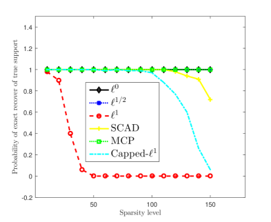
Figure 1: The exact support recovery probability of the solution selected by (16) for Example 5.1.

In the next experiment, we compare Algorithm 2 with an existing general iterative shrinkage and thresholding algorithm (GIST) [28] (available online at http://www.public.asu.edu/~jye02/Software/GIST/). We also compare its efficiency with GLMNET, one of the fastest lasso solvers currently available. We run GIST and GLMNET along the same path that is used in UPDASC with the tuning parameter selection rule (16).

Example 5.2.

We consider the following three different problem settings:

• The matrix $\Psi\in\mathbb{R}^{500\times 5000}$ is generated according to setting (i), and the signal $x^{{\dagger}}$ contains $20$ nonzero elements.

• The matrix $\Psi\in\mathbb{R}^{1000\times 10000}$ is is generated according to setting (ii) and the signal $x^{{\dagger}}$ contains $50$ nonzero elements.

• The matrix $\Psi\in\mathbb{R}^{1000\times 100000}$ is generated according to setting (i) with $\mu=0$, and the signal $x^{{\dagger}}$ contains $50$ nonzero elements.

The performance is evaluated in terms of average CPU time (in seconds) and average relative error defined as $\frac{\|x_{\hat{\lambda}}-x^{{\dagger}}\|}{\|x^{{\dagger}}\|}$, which are computed based on 10 independent realizations of the problem setup. The results are summarized in Tables 3-5.

Table 3: Results for Example 5.2(a), CPU time in seconds and relative error (RE)

	UPDASC			GIST			GLMNET
	time	RE		time	RE		time	RE
$\ell^{0}$	0.15	4.70e-3		-	-		-	-
$\ell^{1/2}$	0.13	4.60e-3		-	-		-	-
SCAD	0.10	4.50e-3		2.07	4.50e-3		-	-
MCP	0.09	4.50e-3		2.13	4.50e-3		-	-
capped-$\ell^{1}$	0.09	4.50e-3		1.38	4.50e-3		-	-
lasso	-	-		-	-		0.23	3.76e-2

Table 4: Results for Example 5.2(b), CPU time in seconds and relative error (RE)

	UPDASC			GIST			GLMNET
	time	RE		time	RE		time	RE
$\ell^{0}$	0.60	3.10e-3		-	-		-	-
$\ell^{1/2}$	0.42	3.30e-3		-	-		-	-
SCAD	0.32	3.10e-3		7.75	3.10e-3		-	-
MCP	0.31	3.10e-3		7.80	3.10e-3		-	-
capped-$\ell^{1}$	0.31	3.10e-3		4.67	3.10e-3		-	-
lasso	-	-		-	-		1.06	4.20e-2

Table 5: Results for Example 5.2(c), CPU time in seconds and relative error (RE)

	UPDASC			GIST			GLMNET
	time	RE		time	RE		time	RE
$\ell^{0}$	5.20	3.40e-3		-	-		-	-
$\ell^{1/2}$	3.76	3.50e-3		-	-		-	-
SCAD	2.60	3.40e-3		75.5	3.40e-3		-	-
MCP	2.59	3.40e-3		75.9	3.40e-3		-	-
capped-$\ell^{1}$	2.60	3.40e-3		13.6	4.65e-1		-	-
lasso	-	-		-	-		12.4	6.16e-2

Since GIST does not support $\ell^{\tau},\tau\in[0,1)$, we do not present the corresponding results, indicated by $-$ in the tables. For all three cases, the proposed UPDASC is much faster than GIST and GLMNET (on average by a factor of ten-thirty and two-five when compared with GIST and GLMNET, respectively). While the reconstruction errors by the proposed UPDAS algorithm is almost identical with that by GIST (except the capped-$\ell^{1}$ in case (c), where, our result is 100 times smaller than GIST) and about ten times smaller than that for GLMNET. This is attributed to its local superlinear convergence, which we shall examine more closely below. These numerical results show clearly the huge potential of the proposed UPDASC algorithm for nonconvex sparse recovery.

We now examine the continuation strategy and local supperlinear convergence of the algorithm.

Example 5.3.

The matrix $\Psi\in\mathbb{R}^{200\times 1000}$ is generated according to (i), and the signal $x^{{\dagger}}$ contains $20$ nonzero elements and $\sigma=0.1$.

The convergence history of Algorithm 2 for Example 5.3 is shown in Fig. 2. In the figure, the notation $A$ and $A_{s}$ refer respectively to the exact active set $\textrm{supp}(x^{{\dagger}})$ and the approximate one $\textrm{supp}(x_{\lambda_{s}})$, where $x_{\lambda_{s}}$ is the solution to the $\lambda_{s}$-problem. It is observed that the size $|A_{s}|$ increases monotonically as the iteration proceeds. At each $\lambda_{s+1}$, with the solution $x_{\lambda_{s}}$ as the initial guess, Algorithm 1 generally converges within three iterations for all five nonconvex penalties, cf., Fig. 2, which shows clearly the highly desirable local superlinear convergence of the algorithm. Hence, the coverall procedure in Algorithm 2 is very efficient.

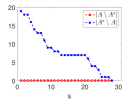
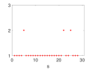
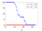
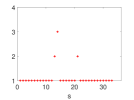
(a) $\ell^{0}$		(b) $\ell^{1/2}$
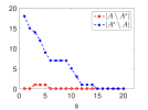
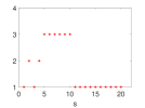
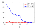
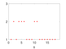
(d) SCAD		(e) MCP
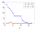
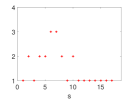
(c) capped-$\ell^{1}$

Figure 2: Convergence behavior of Algorithm 2 for Example 5.3: the variation of the active sets (left panel), and the number of iterations needed for each $\lambda_{s}$-problem (right panel). In the left panel, the vertical axis is the number of iterations, and in the right panel, the vertical axis is the size of the support. The horizontal axis in both panels is the index of the grid point in the solution path.

Four (bridge, capped $\ell^{1}$, SCAD and MCP) of the penalties in Table 1 have a free parameter $\tau$ that controls their concavity. Our next experiment examines the sensitivity of the algorithm with respect to the concavity parameter $\tau$.

Example 5.4.

The matrix $\Psi\in\mathbb{R}^{400\times 1000}$ is generated according to setting (i), and the true signal $x^{{\dagger}}$ contains $10$ nonzero elements with $M=100$.

We evaluate Algorithm 2 by CPU time (in seconds), relative error (in the $\ell^{2}$-norm) and absolute $\ell^{\infty}$ error ($\|x_{\hat{\lambda}}-x^{{\dagger}}\|_{\infty}$) computed from ten independent realizations of the problem setup. The CPU time is fairly robust with respect to the concavity parameter $\tau$, cf. Table 6. Further, the reconstruction error varies little with the parameter $\tau$, indicating the robustness of the penalized models. Interestingly, the reconstruction errors are largely comparable across different penalties.

The consistency results in Theorem 4.1 employ the assumption that the matrix $\Psi$ satisfies the RIP assumption 4.1, which in turn implies that there can only exist very weak correlations among the columns of the matrix $\Psi$. The next experiment examines the robustness of UPDASC with respect to the correlation parameter $\mu$ in data generation setting (i).

Example 5.5.

The matrix $\Psi\in\mathbb{R}^{300\times 1000}$ is generated according to setting (i) with $\mu=0.1:0.2:0.7$, and the true signal $x^{{\dagger}}$ contains $10$ nonzero elements.

Table 6: Results for Example 5.4: sensitivity analysis.

(a) bridge					(b) capped-$\ell^{1}$
$\tau$	Time	RE	AE		$\tau$	Time	RE	AE
$0$	4.40e-2	5.44e-4	4.62e-2		$1.1$	4.86e-2	5.01e-4	4.23e-2
$0.2$	3.79e-2	5.03e-4	4.26e-2		$1.5$	3.59e-2	5.06e-4	4.23e-2
$0.4$	3.47e-2	5.54e-4	4.75e-2		$5$	3.70e-2	5.17e-4	4.23e-2
$0.6$	3.27e-2	5.99e-4	4.85e-2		$10$	3.46e-2	5.25e-4	7.20e-2
$0.8$	2.88e-2	8.44e-4	5.93e-2		$30$	3.58e-2	1.40e-3	1.11e-1
(c) SCAD					(d) MCP
$\tau$	Time	RE	AE		$\tau$	Time	RE	AE
$2.1$	5.72e-2	5.03e-4	4.23e-2		$1.1$	6.30e-2	5.03e-4	4.23e-2
$3.7$	4.70e-2	5.03e-4	4.23e-2		$2.7$	5.07e-2	5.03e-4	4.23e-2
$5$	4.31e-2	5.03e-4	4.23e-2		$5$	4.90e-2	5.03e-4	4.23e-2
$10$	4.33e-2	5.03e-4	4.23e-2		$10$	4.87e-2	5.03e-4	4.24e-2
$30$	4.34e-2	8.66e-4	4.24e-2		$30$	5.32e-2	8.87e-4	7.37e-2

The consistency results in Theorem 4.1 rely on the assumption that $\Psi$ satisfies the RIP i.e., Assumption 4.1, which in turn implies there can only be very weak correlations among the columns of $\Psi$. The next experiment examines the robustness of UPDASC on the correlation parameter $\mu$ in data generation setting (i).

Example 5.6.

The matrix $\Psi\in\mathbb{R}^{300\times 1000}$ is generated according to setting (i) with $\mu=0.1:0.2:0.9$, and the true signal $x^{{\dagger}}$ contains $10$ nonzero elements.

Like before, we evaluate Algorithm 2 (i.e., UPDASC) by CPU time (in seconds), relative error (in the $\ell^{2}$-norm), which are computed from ten independent realizations of the problem setup. Table 7 presents both CPU time (in second) and reconstruction error are fairly robust with respect to the correlation parameter $\mu$ ranging from $0.1$ to $0.9$.

Table 7: Results for Example 5.6: robustness on $\mu$.

$\ell^{0}$			bridge			capped-$\ell^{1}$			SCAD			MCP
$\mu$	Time	RE		Time	RE		Time	RE		Time	RE		Time	RE
$0.1$	2.80e-2	6.00e-3		2.40e-2	6.00e-3		3.08e-2	5.70e-3		4.52e-2	5.70e-3		3.62e-2	5.70e-3
$0.3$	1.88e-2	5.00e-3		1.69e-2	5.00e-3		1.55e-2	5.70e-3		2.41e-2	5.70e-3		1.88e-2	5.70e-3
$0.5$	1.88e-2	5.00e-3		1.41e-2	5.00e-3		1.56e-2	5.70e-3		2.29e-2	5.70e-3		1.90e-2	5.70e-3
$0.7$	1.75e-2	6.02e-3		1.56e-2	6.02e-3		1.51e-2	5.90e-3		2.13e-2	5.90e-3		1.96e-2	5.90e-3
$0.9$	1.95e-2	6.63e-3		1.60e-2	6.75e-3		1.55e-2	6.63e-3		2.15e-2	6.63e-3		1.99e-2	6.63e-3

Finally, we illustrate Algorithm 2 on a genome-wide association study (GWAS) dataset.

Example 5.7.

This test applies UPDASC to high-density lipoprotein (HDL) in NFBC1966 study [57]. The NFBC1966 data set contains information for 5,402 individuals with a selected list of phenotypic data including HDL and 364,590 single nucleotide polymorphisms (SNPs). We perform strict quality control on data using PLINK [56]. In the experiments, we exclude individuals having discrepancies between the reported sex and the sex determined from the X chromosome, and exclude SNPs with a minor allele frequency less than 1$\%$, having missing values in more than 1$\%$ of the individuals or with a Hardy-Weinberg equilibrium p-value below 0.0001. After conducting strict quality control, 5,123 individuals with 9,114 SNPs in NFBC1966 on chromosome 16 are retained for the further analysis.

The numbers of SNPs identified across $\ell^{0}$, $\ell^{1/2}$, SCAD, MCP and capped-$\ell^{1}$ are listed in Table 8, where the diagonals on the table are numbers of variables selected via different penalties and off diagonals are the numbers of variables in the intersections of support sets determined across two different penalties. The solution pathes of different penalties are presented in Fig. 3. Among all identified SNPs, rs3764261 and rs7499892 near gene CETP are found to be associated with HDL in prior studies [67, 68, 64].

Table 8: Results for Example 5.7.

	$\ell^{0}$	$\ell^{1/2}$	SCAD	MCP	capped-$\ell^{1}$
$\ell^{0}$	18	10	18	18	18
$\ell^{1/2}$		11	10	10	10
SCAD			27	27	27
MCP				27	27
capped-$\ell^{1}$					27

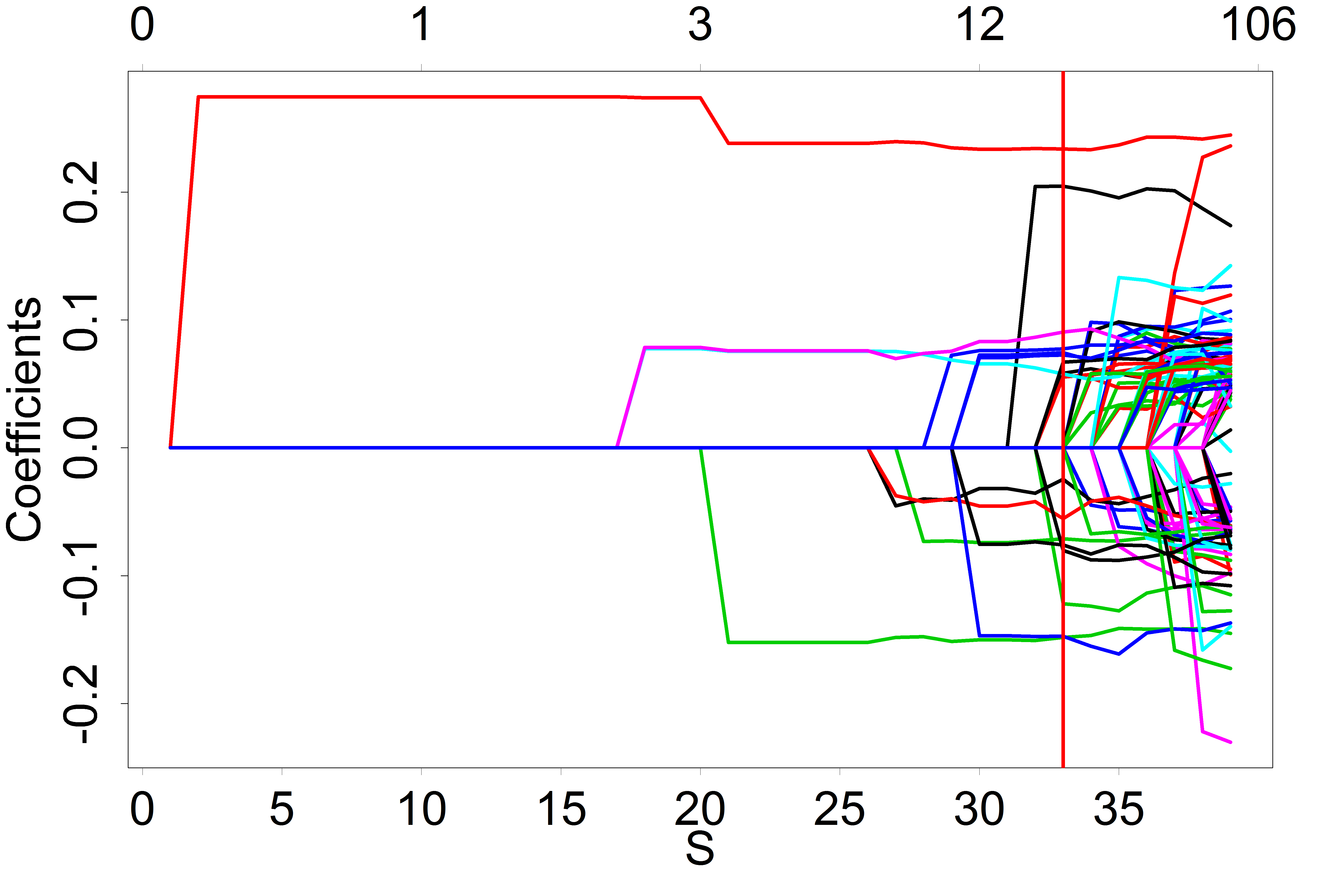
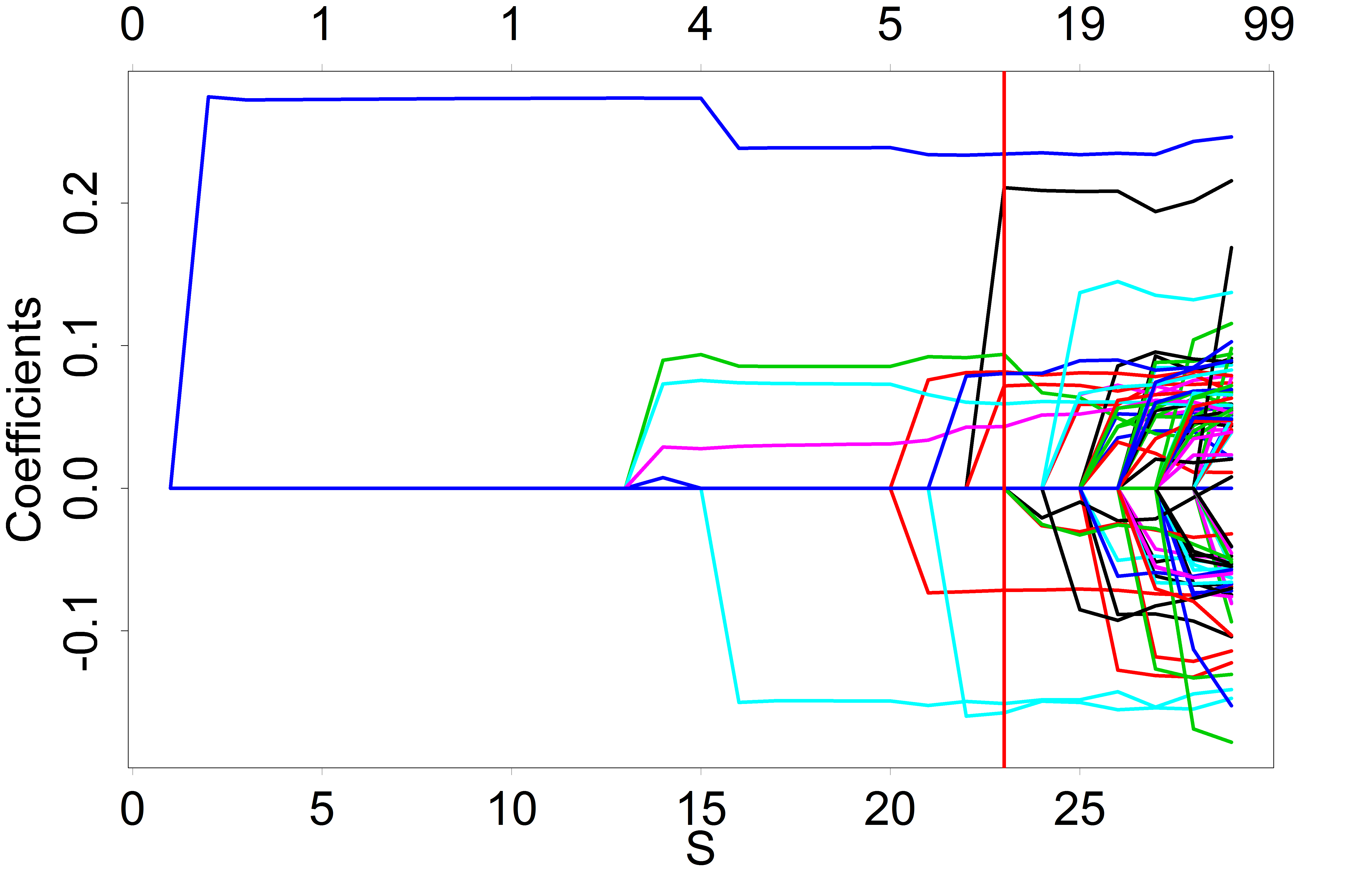
(a) $\ell^{0}$	(b) $\ell^{1/2}$
(c) SCAD	(d) MCP
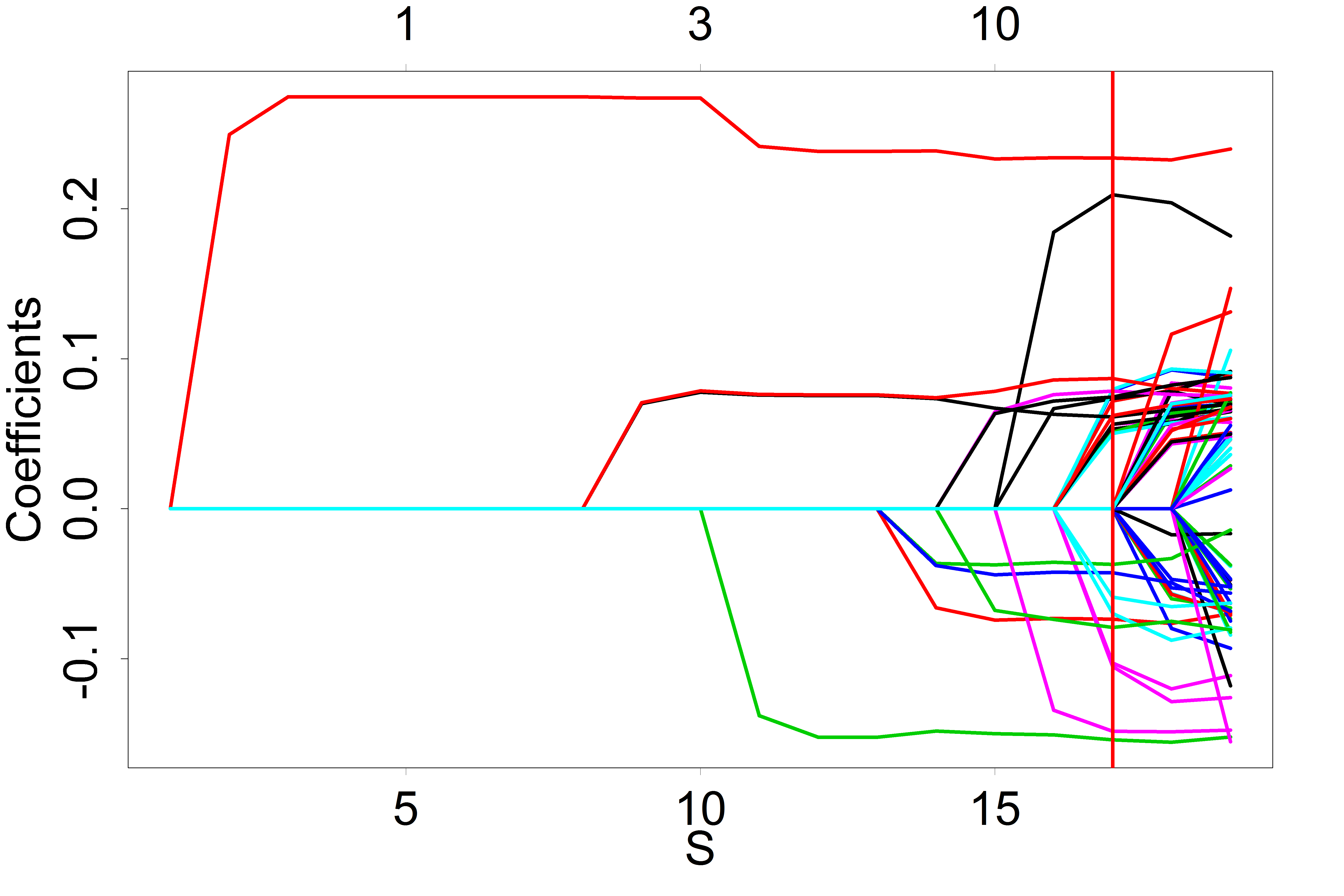
(e) capped-$\ell^{1}$

Figure 3: Solution path for example 5.7

6 Conclusions

In this work, we have developed a unified PDAS algorithm for a class of popular nonconvex penalized regression problems arising in high-dimensional statistics and sparse signal recovery, including the $\ell^{0}$, bridge, capped-$\ell^{1}$, smoothly clipped absolute deviation and minimax concave penalty. Theoretically, we established the existence of a global minimizer, and derived a necessary optimality condition for a global minimizer, based on the associated thresholding operator. The solutions to the necessary optimality condition are always coordinate-wise minimizers, and further, we provided verifiable sufficient conditions for a coordinate-wise minimizer to be a local minimizer. Meanwhile, the necessary optimality condition and the active set can be reformulated using both primal and dual variables, which lends itself to a primal-dual active set algorithm. One distinct feature of the algorithm is that at each iteration, it involves only solving a least-squares problem on the active set, which is usually of much smaller size, and merits a local superlinear convergence, and thus when coupled with a continuation strategy, the procedure is very efficient and accurate. The global convergence of the overall UPDASC was shown under suitable restricted isometry property on the design matrix. The efficiency and accuracy of UPDASC combined with a new tuning parameter selection rule are clearly demonstrated by extensive numerical experiments, including real data.

There are several avenues for further study. First, for very ill-conditioned design matrices, which are characteristic of high-dimensional problems with highly correlated covariates, the linear systems involved in the PDAS algorithm can be challenging to solve directly, and extra regularization might be necessary. The extra regularization can be achieved by either penalization or early stopping. This motivates further researches on related theoretical issues, especially stability and error estimates. Second, in some practical applications, the design matrix $\Psi$ is only implicitly given where only matrix-vector multiplication is available. This necessitates developing iterative linear solvers, and the study of inexact inner iterations, e.g., especially convergence properties. Last, the extensions of the UPDASC algorithm to structured sparsity, e.g., group sparsity penalty and the matrix analogues, are also of immense current interest.

Supplementary Materials

Appendix: The supplementary materials contain the proofs of the theoretical results and one counterexample.

Appendix A Appendix

In the appendix, we prove Propositions 2.1 and 3.1 and Theorems 3.1 and 4.1. and give one counterexample to shed light on the conditions in Theorem 3.1.

A.1 Proof of Proposition 2.1

First, we show a technical lemma.

Lemma A.1.

Let the function $\rho(t):\mathbb{R}\to\mathbb{R}^{+}\cup\{0\}$ satisfy:

• $\rho$ is even with $\rho(0)=0$, nondecreasing for $t\geq 0$, and lower semi-continuous.

• $\rho(t)$ is a constant when $|t|\geq t_{0}$ for some $t_{0}>0$.

Then for any given subspace ${\cal N}\subset\mathbb{R}^{p}$, the following statements hold.

• For any $x\in\mathcal{N}^{\perp}$, there exists an element $z\in\mathcal{N}$ such that $\sum_{i=1}^{p}\rho(x_{i}+z_{i})=\inf_{z\in{\cal N}}\sum_{i=1}^{p}\rho(x_{i}+z_{i})$.

• Let $SE(x)=\mathop{\mathrm{missing}}{arg}\min_{z\in\cal N}\sum_{i=1}^{p}\rho(x_{i}+z_{i})$. Then the function $h:{\cal N}^{\perp}\mapsto\mathbb{R}$, $h(x)=\inf_{z\in SE(x)}\|z\|$ maps a bounded set to a bounded set.

Proof.

To show part (a), let $m$ be the dimension of $\cal N$, and $S\in\mathbb{R}^{p\times m}$ be a column orthonormal matrix whose columns form a basis of $\mathcal{N}$. We denote the rows of $S$ by $\{\tilde{s}_{i}\}_{i=1}^{p}$. Then any $z\in\cal{N}$ can be written as $z=Sw$ for some $w\in\mathbb{R}^{m}$. Let $\{w_{k}\}\subset\mathbb{R}^{m}$ be a minimizing sequence to $\inf_{z\in\cal N}\sum_{i=1}^{p}\rho(x_{i}+z_{i})$ under the representation $z=Sw$. We claim that there exists a $w\in\mathbb{R}^{m}$ such that

$$\sum_{i=1}^{p}\rho(x_{i}+(Sw)_{i})\leq\lim_{k\rightarrow\infty}\sum_{i=1}^{p}\rho(x_{i}+(Sw_{k})_{i}).$$

First, if there is a bounded subsequence of $\{w_{k}\}$, the existence of a minimizer follows from the lower semicontinuity of $\rho$. Hence we assume that $\|w_{k}\|\rightarrow\infty$ as $k\to\infty$. Then we check the scalar sequences $\{w_{k}\cdot\tilde{s}_{i}\}_{k}$, $i\in\mathbb{I}\equiv\{1,...,p\}$. For any $i\in\mathbb{I}$, if there is a bounded subsequence of $\{w_{k}\cdot\tilde{s}_{i}\}$, we may pass to a convergent subsequence and relabel it to be the whole sequence. In this way, we divide the index set $\mathbb{I}$ into two disjoint subsets $\mathbb{I}^{\prime}$ and $\mathbb{I}^{\prime\prime}$ such that for every $i\in\mathbb{I}^{\prime}$, $w_{k}\cdot\tilde{s}_{i}$ converges, whereas for every $i\in\mathbb{I}^{\prime\prime}$, $|w_{k}\cdot\tilde{s}_{i}|\rightarrow\infty$. Let $\mathcal{L}=\mathrm{span}\{\tilde{s}_{i}\}_{i\in\mathbb{I}^{\prime}}$, and decompose $w_{k}$ into $w_{k}=w_{k,\cal L}+w_{k,\cal L^{\perp}}$, with $w_{k,\cal L}\in\mathcal{L}$ and $w_{k,\cal L^{\perp}}\in\mathcal{L}^{\perp}$.

If the index set $\mathbb{I}^{\prime}$ is empty, then by the monotonicity of the function $\rho(t)$, one can verify directly that the zero vector $0$ is a minimizer. Otherwise, by the definition of $\mathbb{I}^{\prime}$ and the monotonicity of $\rho(t)$, for any $i\in\mathbb{I}^{\prime}$, $w_{k}\cdot\tilde{s}_{i}=w_{k,\cal L}\cdot\tilde{s}_{i}$, and for any $i\in\mathbb{I}^{\prime\prime}$, $\limsup_{k\rightarrow\infty}\rho(x_{i}+w_{k,\mathcal{L}}\cdot\tilde{s}_{i})\leq\lim_{k\rightarrow\infty}\rho(x_{i}+w_{k}\cdot\tilde{s}_{i})$. Hence $\{w_{k,\cal L}\}$ is also a minimizing sequence. Next we prove that $\{w_{k,\cal L}\}$ is bounded. To this end, we let $M$ be the submatrix of $S$, consisting of rows whose indices are listed in $\mathbb{I}^{\prime}$. It follows from the definition of $w_{k,\cal L}$ and the convergence of $w_{k,\cal L}\cdot\tilde{s}_{i}$ for $i\in\mathbb{I}^{\prime}$ that $w_{k,\cal L}\in{\cal L}=\mbox{Range}(M^{t})$ and $Mw_{k,\cal L}$ is bounded. Now let $M=U^{t}\Sigma V$ be the singular value decomposition of $M$. Then for any $w\in\mbox{Range}(M^{t})$, i.e., $w=M^{t}q$, there holds

$$\|Mw\|^{2}=\|\Sigma\Sigma^{t}Uq\|^{2}=\sum_{\sigma_{i}>0}\sigma_{i}^{4}(Uq)_{i}^{2}\geq\sigma_{M}^{2}\sum_{\sigma_{i}>0}\sigma_{i}^{2}(Uq)_{i}^{2}=\sigma_{M}^{2}\|\Sigma^{t}Uq\|^{2}=\sigma_{M}^{2}\|w\|^{2},$$

where $\sigma_{M}$ is the smallest nonzero singular value of $M$. Hence the sequence $\{w_{k,\cal L}\}$ is bounded, from which the existence of a minimizer follows. This shows part (a).

By the construction in part (a), the set $SE(x)$ is nonempty, and by the lower semi-continuity of $\rho$, it is closed. Hence, there exists an element $z(x)\in SE(x)$ such that $\|z(x)\|=\inf_{z\in SE(x)}\|z\|$. We claim that the map $x\mapsto z(x)$ is bounded. To this end, let $D=\|x\|_{\infty}$, and recall the representation $z=Sw$ and $(x+z)_{i}=x_{i}+w\cdot\tilde{s}_{i}$. Denote by $\mathbb{I}^{\prime}=\{i\in\mathbb{I}:|w\cdot\tilde{s}_{i}|\leq D+t_{0}\}$, and let ${\cal L}=\mathrm{span}\{\tilde{s}_{i}\}_{i\in\mathbb{I}^{\prime}}$, $w=w_{\cal L}+w_{\cal L^{\perp}}$, with $w_{\mathcal{L}}\in{\cal L}$ and $w_{\cal L^{\perp}}\in{\cal L}^{\perp}$. Then the argument in part (a) yields

$$\left.\begin{array}[]{ll}\tilde{s}_{i}\cdot w_{\mathcal{L}}=\tilde{s}_{i}\cdot w&i\in\mathbb{I}^{\prime}\\ \rho(x_{i}+\tilde{s}_{i}\cdot w_{\mathcal{L}})\leq\rho(t_{0})=\rho(x_{i}+\tilde{s}_{i}\cdot w)&i\in\mathbb{I}\backslash\mathbb{I}^{\prime}\end{array}\right\}\Rightarrow\tilde{z}(x)=Sw_{\mathcal{L}}(x)\in SE(x),$$

and

$$\|Sw_{\mathcal{L}}(x)\|\leq C_{\mathbb{I}^{\prime}}(D+t_{0}),$$

where the constant $C_{\mathbb{I}^{\prime}}$ depends only on the smallest nonzero singular value of the submatrix whose rows are given by $\tilde{s}_{i}$, $i\in\mathbb{I}^{\prime}$. Therefore,

$$\sup\limits_{\|x\|_{\infty}\leq D}\inf\limits_{z\in SE(x)}\|z\| =\sup\limits_{\|x\|_{\infty}\leq D}\|{z}(x)\|\leq\sup\limits_{\|x\|_{\infty}\leq D}\|\tilde{z}(x)\|$$

$$=\sup\limits_{\|x\|_{\infty}\leq D}\|Sw_{\mathcal{L}}(x)\|\leq\sup\limits_{\mathbb{I}^{\prime}}C_{\mathbb{I}^{\prime}}(D+t_{0}).$$

The factor $\sup_{\mathbb{I}^{\prime}}C_{\mathbb{I}^{\prime}}$ is over finitely many numbers, which concludes the proof. ∎

Proof of Proposition 2.1

Proof.

We discuss the cases separately.

(i) bridge. The proof is straightforward due to the coercivity of the penalty.

(ii) $\ell^{0}$, capped-$\ell^{1}$, SCAD and MCP. First, all these penalties satisfy the assumptions in Lemma A.1. Let $\mathcal{N}=\mathrm{Ker}(\Psi)$, then $\Psi$ is coercive over $\mathcal{N}^{\perp}$, and $\mathrm{Ker}(\Psi)^{\perp}=\mathrm{Range}(\Psi^{t})$. Since the functional $J$ is bounded from below by zero, the infimum $\textrm{INF}=\inf J(x)$ exists and it is finite; further, by the very definition of the infimum INF, there exists a minimizing sequence, denoted by $\{x^{k}\}\subset\mathbb{R}^{p}$, to (3), i.e., $\lim_{k\rightarrow\infty}J(x^{k})=\textrm{INF}$ [27, Section 39, pp. 193]. We decomposed $x^{k}$ into $x^{k}=P_{\mathcal{N}}x^{k}+P_{\mathcal{N}^{\perp}}x^{k}=:u^{k}+v^{k}$, where $P_{\cal N}$ and $P_{{\cal N}^{\perp}}$ denote the orthogonal projection into $\cal N$ and ${\cal N}^{\perp}$, respectively. By the construction of the set $SE(v^{k})$ in the proof of Lemma A.1, with the minimum-norm element $\tilde{u}^{k}\in SE(v^{k})$ in place of $u^{k}$, the sequence $\{v^{k}+\tilde{u}^{k}\}$ is still minimizing. By the coercivity, $\{v^{k}\}$ is bounded, and hence $\{\tilde{u}^{k}\}$ is also bounded by Lemma A.1(b). Upon passage to a convergent subsequence, the lower semi-continuity of $J$ implies the existence of a minimizer. ∎

A.2 Proof of Proposition 3.1

We first prove Lemma 3.2 and Lemma 3.3.

Proof of Lemma 3.2

Proof.

We compute $(t^{*},T^{*})$ for the five penalties separately.

(i) $\ell^{0}$. $g(t)=\frac{t}{2}+\frac{\lambda}{t}$ for $t>0$ and $g(0)=+\infty$. Hence $t^{*}=\sqrt{2\lambda}$ and $T^{*}=g(t^{*})=\sqrt{2\lambda}$.

(ii) bridge. $g(t)=\frac{t}{2}+\lambda t^{\tau-1}$ for $t>0$ and $g(0)=+\infty$. Direct computation gives $t^{*}=\left(2\lambda(1-\tau)\right)^{\frac{1}{2-\tau}}$, and $T^{*}=g(t^{*})=(2-\tau)\left[2(1-\tau)\right]^{\frac{\tau-1}{2-\tau}}\lambda^{\frac{1}{2-\tau}}$.

(iii) capped-$\ell^{1}$. Then the function $g(t)$ is given by

$$g(t)=\frac{t}{2}+\left\{\begin{array}[]{ll}\frac{\lambda^{2}\tau}{t},&t\geq\lambda\tau,\\[4.30554pt] \lambda,&0\leq t\leq\lambda\tau.\end{array}\right.$$

In the interval $[0,\lambda\tau]$, $0$ is the minimizer of $g(t)$ with a minimum value $\lambda$, whereas in the interval $[\lambda\tau,\infty)$, the minimum value is $\lambda\sqrt{2\tau}$, which is greater than $\lambda$. Hence $t^{*}=0$, and $T^{*}=\lambda$.

(iv) SCAD. Then the function $g(t)$ is given by

$$g(t)=\frac{t}{2}+\left\{\begin{array}[]{ll}\frac{\lambda^{2}(\tau+1)}{2t},&t\geq\lambda\tau,\\[5.16663pt] \frac{\lambda\tau t-\frac{1}{2}(t^{2}+\lambda^{2})}{(\tau-1)t},&\lambda\leq t\leq\lambda\tau,\\[5.16663pt] \lambda,&0\leq t\leq\lambda.\end{array}\right.$$

It can be verified directly that the minimizer of $g(t)$ in the intervals $[0,\lambda]$, $[\lambda,\lambda\tau]$, $[\lambda\tau,\infty)$ is given by $0$, $\lambda$, $\lambda\sqrt{\tau+1}$, respectively. Hence $t^{*}=0$, and $T^{*}=\lambda$.

(v) MCP. Then the function $g(t)$ is given by

$$g(t)=\frac{t}{2}+\left\{\begin{array}[]{ll}\frac{\lambda^{2}\tau}{2t},&t\geq\lambda\tau,\\[5.16663pt] \lambda-\frac{t}{2\tau},&0\leq t\leq\lambda\tau.\end{array}\right.$$

Analogous to the case of the SCAD, we can obtain $t^{*}=0$, and $T^{*}=\lambda$. ∎

Proof of Lemma 3.3

Proof.

By the lower-semicontinuity and coercivity of the function ${(u-v)^{2}}/{2}+\rho(u)$, it has at least one minimizer. Next one observes that

$$u^{\ast}\in\mathop{\textrm{missing}}{argmin}_{u\in\mathbb{R}}\left({(u-v)^{2}}/{2}+\rho(u)\right)\quad\Leftrightarrow\quad u^{\ast}\in\mathop{\textrm{missing}}{argmin}_{u\in\mathbb{R}}\left({u^{2}}/{2}-uv+\rho(u)\right).$$

First, if $u^{\ast}=0$, then for any $u\neq 0$, ${u^{2}}/{2}-uv+\rho(u)=u(g(u)-v)$, which implies that $u$ and $g(u)-v$ have the same sign. That is,

$$u>0\Rightarrow g(u)-v\geq 0,\quad\forall u>0,\quad\mbox{ then }v\leq\inf\limits_{u>0}g(u)=T^{*},$$

and

$$u<0\Rightarrow g(u)-v\leq 0,\quad\forall u<0,\quad\mbox{ then }-v\leq\inf\limits_{u<0}-g(u)=\inf\limits_{u<0}g(-u)=T^{*}.$$

From these observations it follows that $|v|\leq T^{*}$. This shows assertion (a). Second, let $G(u)=u(g(u)-v)$ for $u\neq 0$ and $G(0)=0$. For $|v|<T^{*}$, since

$$u>0\Rightarrow g(u)\geq T^{*}>v\quad\mbox{and}\quad u<0\Rightarrow g(u)=-g(-u)\leq-T^{*}<v,$$

then $G(u)>0$ when $u\neq 0$, which implies $0$ is the only minimizer. This shows (b). Last, for $|v|=T^{*}$, by arguing analogously to (b) for $u>0$ and $u<0$, we have $G(u)\geq 0$. Then $u^{\ast}$ satisfies that $G(u^{\ast})=0$, i.e., $u^{\ast}=0$ or $g(u^{\ast})={\mathrm{sgn}}(v)T^{*}$. ∎

Now we can state the proof of Proposition 3.1.

Proof.

We discuss only the case $v>0$, for which $u^{*}\geq 0$. The case $v<0$ can be treated similarly.

(i) $\ell^{0}$. By Lemma 3.3, if $|v|>T^{*}$, then $u^{*}\neq 0$ which implies the minimizer $u^{*}$ is $v$, from which the formula of $S_{\lambda}^{\ell^{0}}$ follows (see also [40]).

(ii) bridge. Let $G(u)=\frac{u^{2}}{2}+\lambda u^{\tau}-uv$ for $u\geq 0$. Its first- and second derivatives are given by

$$G^{\prime}(u)=u+\lambda\tau u^{\tau-1}-v\quad\mbox{and}\quad G^{\prime\prime}(u)=1+\lambda\tau(\tau-1)u^{\tau-2}.$$

Clearly, $G^{\prime}(u)$ is convex with $G^{\prime}(0+)=G^{\prime}(+\infty)=+\infty$. Hence, $G^{\prime}(u)$ has at most two real roots, and $G(u)$ is either monotonically increasing or has three monotone intervals. This and Lemma 3.3 yield the expression $S_{\lambda,\tau}^{\ell^{\tau}}$. Generally there is no closed-form expression for $S^{\ell^{\tau}}_{\lambda,\tau}(v)$. For $|v|>T^{*}$, the unique minimizer to $G(u)$ is the larger root of $G^{\prime}(u)$ (the other root is a local maximizer) (see also [40, 28]).

(iii) capped-$\ell^{1}$. Let

$$G(u)=\left\{\begin{array}[]{ll}\frac{u^{2}}{2}-uv+\lambda^{2}\tau,&u\geq\lambda\tau,\\[5.16663pt] \frac{u^{2}}{2}-uv+\lambda u,&0\leq u\leq\lambda\tau.\end{array}\right.$$

By Lemma 3.3, for $|v|\leq\lambda$, we have $u^{*}=0$. We then assume $v>\lambda$. Simple computation shows

$$S^{*}_{1} :=\min_{u\geq\lambda\tau}G(u)=\lambda^{2}\tau-{v^{2}}/{2}\mbox{ at }u=v,$$

$$S_{2}^{*} :=\min_{u\in[0,\lambda\tau]}G(u)=-{(v-\lambda)^{2}}/{2}\mbox{ at }u=v-\lambda.$$

Then we have

$$\left\{\begin{array}[]{ll}v>\lambda(\tau+\frac{1}{2})\Rightarrow S_{1}^{*}<S_{2}^{*},&u^{*}=v>\lambda\tau,\\[5.16663pt] v<\lambda(\tau+\frac{1}{2})\Rightarrow S_{1}^{*}>S_{2}^{*},&u^{*}=v-\lambda<\lambda\tau,\\[5.16663pt] v=\lambda(\tau+\frac{1}{2})\Rightarrow S_{1}^{*}=S_{2}^{*},&u^{*}=\lambda\tau\pm\frac{\lambda}{2},\end{array}\right.$$

whence follows the thresholding operator $S^{c\ell^{1}}_{\lambda,\tau}$ (see also [28]).

(iv) SCAD. We define

$$G(u)=\left\{\begin{array}[]{ll}G_{1}(u)\triangleq\frac{u^{2}}{2}-uv+\frac{\lambda^{2}(\tau+1)}{2},&u\geq\lambda\tau,\\[5.59721pt] G_{2}(u)\triangleq\frac{u^{2}}{2}-uv+\frac{\lambda\tau u-\frac{1}{2}(u^{2}+\lambda^{2})}{\tau-1},&\lambda\leq u\leq\lambda\tau,\\[5.59721pt] G_{3}(u)\triangleq\frac{u^{2}}{2}-uv+\lambda u,&0\leq u\leq\lambda.\end{array}\right.$$

By Lemma 3.3, $|v|\leq\lambda\Rightarrow u^{*}=0$. We then assume $v>\lambda$. The three quadratic functions $G_{i}(u)$ achieve their minimum at $u=v$, $u=\frac{(\tau-1)v-\lambda\tau}{\tau-2}$ and $u=v-\lambda$, respectively. Next we discuss the three cases separately. First, if $v\geq\lambda\tau$, then $\frac{(\tau-1)v-\lambda\tau}{\tau-2}\geq\lambda\tau$, which implies that $G_{2}(u)$ is decreasing on the interval $[\lambda,\lambda\tau]$, it reaches its minimum at $\lambda\tau$. Similarly, $v-\lambda\geq\lambda$ implies that $G_{3}(u)$ reaches its minimum over the interval $[0,\lambda]$ at $\lambda$. Hence

$$\min\limits_{0\leq u\leq\lambda}G_{3}(u) =G_{3}(\lambda)=G_{2}(\lambda)\geq\min\limits_{\lambda\leq u\leq\lambda\tau}G_{2}(u)=G_{2}(\lambda\tau)=G_{1}(\lambda\tau)\geq\min\limits_{u\geq\lambda\tau}G_{1}(u).$$

Second, if $\lambda\tau\geq v\geq 2\lambda$, then $G_{1}$ is increasing on $[\lambda\tau,\infty)$ and $G_{3}$ is decreasing on $[0,\lambda]$, and $\frac{(\tau-1)v-\lambda\tau}{\tau-2}\geq\lambda\tau\in[\lambda,\lambda\tau]$. Hence

$$\min_{0\leq u\leq\lambda}G_{3}(u)=G_{3}(\lambda)=G_{2}(\lambda)\geq\min_{\lambda\leq u\leq\lambda\tau}G_{2}(u),$$

$$\min_{\lambda\leq u\leq\lambda\tau}G_{2}(u)\leq G_{2}(\lambda\tau)=G_{1}(\lambda\tau)=\min_{u\geq\lambda\tau}G_{1}(u).$$

Third, if $2\lambda\geq v\geq\lambda$, similar argument gives that

$$\min\limits_{0\leq u\leq\lambda}G_{3}(u) \leq G_{3}(\lambda)=G_{2}(\lambda)=\min\limits_{\lambda\leq u\leq\lambda\tau}G_{2}(u)\leq G_{2}(\lambda\tau)=G_{1}(\lambda\tau)=\min\limits_{u\geq\lambda\tau}G_{1}(u).$$

This yields the thresholding operator $S_{\lambda,\tau}^{\mathrm{scad}}$ (see also [5, 51, 28]).

(v) MCP. Like before, we let

$$G(u)=\left\{\begin{array}[]{ll}\frac{u^{2}}{2}-uv+\frac{1}{2}\lambda^{2}\tau,&u\geq\lambda\tau,\\[5.59721pt] \frac{u^{2}}{2}-uv+\lambda u-\frac{u^{2}}{2\tau},&0\leq u\leq\lambda\tau.\end{array}\right.$$

Similar to case (iv), we obtain the expression for $S_{\lambda,\tau}^{\mathrm{mcp}}$ (see also [5, 51, 28]). ∎

A.3 Proof of Theorem 3.1

Proof.

We prove Theorem 3.1 by establishing the inequality

$$J(x^{*}+\omega)\geq J(x^{*})$$ (17)

for small $\omega\in\mathbb{R}^{p}$, using the optimality condition and thresholding operator.

(i) $\ell^{0}$. By Lemma 3.4 and using the thresholding operator $S_{\lambda}^{\ell^{0}}$, we deduce that for $i\in{\cal A}$, $|x_{i}^{*}|\geq\sqrt{2\lambda}$. Further,

$$0=d^{*}_{{\mathcal{A}}}=\Psi_{{\mathcal{A}}}^{t}(y-\Psi_{\cal A}x^{*}_{\cal A})\quad\Leftrightarrow\quad x^{*}_{{\mathcal{A}}}\in\mathop{\textrm{missing}}{argmin}\tfrac{1}{2}\|\Psi_{{\mathcal{A}}}x_{{\mathcal{A}}}-y\|^{2}.$$ (18)

Now consider a small perturbation $\omega$, with $\|\omega\|_{\infty}<\sqrt{2\lambda}$, to $x^{*}$. It suffices to show (17) for small $\omega$. Recall that $\omega_{\cal I}$ is the subvector of $\omega$ whose entries are listed in the index set $\cal I$. If $\omega_{\mathcal{I}}\neq 0$, then

$$J(x^{*}+\omega)-J(x^{*}) \geq\tfrac{1}{2}\|\Psi x^{*}-y+\Psi\omega\|^{2}-\tfrac{1}{2}\|\Psi x^{*}-y\|^{2}+\lambda\geq\lambda-|(\omega,d^{\ast})|,$$

which is positive for small $\omega$. Meanwhile, if $\omega_{{\mathcal{I}}}=0$, by (18), we deduce (17).

(ii) bridge. First note that on the active set ${\mathcal{A}}$, $|x_{i}^{*}|\geq t^{*}=\left(2\lambda(1-\tau)\right)^{\frac{1}{2-\tau}}$. Next we claim that if the minimizer $u^{*}$ of $G(u)=\tfrac{u^{2}}{2}-uv+\lambda u^{\tau}$ is positive, then $G(u)$ is locally strictly convex around $u^{*}$, i.e., for small $t$ and some $\theta>0$ such that

$$G(u^{*}+t)-G(u^{*})=G(u^{*}+t)-G(u^{*})-G^{\prime}(u^{*})t\geq\theta t^{2}.$$

To see this, we recall that $u^{*}$ is the larger root of $u+\lambda\tau u^{\tau-1}=v$ and $v\geq T^{*}$. By the convexity of $u+\lambda\tau u^{\tau-1}$, $u^{*}(v)$ is increasing in $v$ for $v\geq T^{*}$. Further, by the inequality $u^{*}\geq t^{*}$, we have

$$G^{\prime\prime}(u^{*}) =1-\lambda\tau(1-\tau)(u^{*})^{\tau-2}$$

$$\geq 1-\lambda\tau(1-\tau)(t^{*})^{\tau-2}=1-\tfrac{\tau}{2}.$$

In particular, the function $G(u)$ is locally strictly convex with $\theta=\frac{1}{2}-\frac{\tau}{4}-\epsilon$, for any $\epsilon>0$. Hence for each $i\in{\mathcal{A}}$ and small $t$, there holds

$$J(x^{*}+te_{i})-J(x^{*}) =\tfrac{1}{2}t^{2}+(t\psi_{i},\Psi x^{*}-y)+\lambda|x^{*}_{i}+t|^{\tau}-\lambda|x^{*}_{i}|^{\tau}\geq\theta t^{2},$$

i.e.,

$$-td_{i}^{*}+\lambda|x_{i}^{*}+t|^{\tau}-\lambda|x_{i}^{*}|^{\tau}\geq(\theta-\tfrac{1}{2})t^{2}.$$

Consequently for small $\omega$, we have

$$J(x^{*}+\omega)-J(x^{*}) =\tfrac{1}{2}\|\Psi\omega\|^{2}-(\omega,d^{*})+\sum_{i\in{\mathcal{A}}}\lambda(|x_{i}^{*}+\omega_{i}|^{\tau}-|x_{i}^{*}|^{\tau})+\lambda\sum_{i\in{\mathcal{I}}}|\omega_{i}|^{\tau}$$

$$\geq\tfrac{1}{2}\|\Psi\omega\|^{2}-(\omega_{\cal I},d^{*}_{{\mathcal{I}}})+\lambda\sum_{i\in{\mathcal{I}}}|\omega_{i}|^{\tau}+(\theta-\tfrac{1}{2})\|\omega_{{\mathcal{A}}}\|^{2}.$$

Note the trivial estimates

$$-(\omega_{{\mathcal{I}}},d^{*}_{{\mathcal{I}}})\geq-\sum_{i\in{\mathcal{I}}}|\omega_{i}|\|d^{*}_{\mathcal{I}}\|_{\infty}\quad\mbox{and}\quad\tfrac{1}{2}\|\Psi\omega\|^{2}\geq\tfrac{1}{2}\|\Psi_{{\mathcal{A}}}\omega_{\cal A}\|^{2}+(\omega_{{\mathcal{A}}},\Psi^{t}_{{\mathcal{A}}}\Psi_{{\mathcal{I}}}\omega_{{\mathcal{I}}}).$$

Further, by Young’s inequality, for any $\delta>0$

$$(\omega_{{\mathcal{A}}},\Psi^{t}_{{\mathcal{A}}}\Psi_{{\mathcal{I}}}\omega_{{\mathcal{I}}})\geq-\delta\|\omega_{{\mathcal{A}}}\|^{2}-\tfrac{1}{4\delta}\|\Psi^{t}_{{\mathcal{A}}}\Psi_{{\mathcal{I}}}\omega_{{\mathcal{I}}}\|^{2}\geq-\delta\|\omega_{{\mathcal{A}}}\|^{2}-C_{\delta}\|\omega_{{\mathcal{I}}}\|^{2}.$$

Combing these four estimates together and noting $\theta=\frac{1}{2}-\frac{\tau}{4}-\epsilon$ yields

$$J(x^{*}+\omega)-J(x^{*}) \geq\left(\tfrac{1}{2}\|\Psi_{{\mathcal{A}}}\omega_{{\mathcal{A}}}\|^{2}-(\tfrac{\tau}{4}+\epsilon+\delta)\|\omega_{{\mathcal{A}}}\|^{2}\right)$$

$$\quad+\sum_{i\in{\mathcal{I}}}|\omega_{i}|^{\tau}\left(\lambda-|\omega_{i}|^{1-\tau}\|d^{*}_{\mathcal{I}}\|_{\infty}-C_{\delta}|\omega_{i}|^{2-\tau}\right).$$

The first term is nonnegative if $\epsilon$ and $\delta$ are small and $\Psi$ satisfies (8) with $\sigma(\mathcal{A})>\frac{\tau}{2}$. The sum over ${\mathcal{I}}$ is nonnegative for small $\omega$, thereby showing (17).

The proof of the rest cases is based on the identity

$$J(x^{*}+\omega)-J(x^{*})=\tfrac{1}{2}\|\Psi\omega\|^{2}+\sum_{i}\underbrace{(\rho_{\lambda,\tau}(x_{i}^{*}+\omega_{i})-\rho_{\lambda,\tau}(x_{i}^{*})-\omega_{i}d^{*}_{i})}_{:=s_{i}}.$$ (19)

(iii) capped-$\ell^{1}$. We denote by ${{\mathcal{A}}}_{1}=\{i:|x_{i}^{*}|>\lambda\tau\}$, ${{\mathcal{A}}}_{2}=\{i:\lambda\tau>|x_{i}^{*}|>0\}$. By assumption $\{i:|x_{i}^{*}|=\lambda\tau\}=\emptyset$, hence ${{\mathcal{I}}}=({\cal A}_{1}\cup{\cal A}_{2})^{c}$. The optimality condition for $x^{*}$ and the differentiability of $\rho_{\lambda,\tau}^{c\ell^{1}}(t)$ for $|t|\neq\lambda\tau$ yield $d_{i}^{*}=0$ for $i\in{{\mathcal{A}}}_{1}$, and $d_{i}^{*}=\lambda{\mathrm{sgn}}(x_{i}^{*})$ for $i\in{{\mathcal{A}}}_{2}$. Thus, for $\omega$ small, there holds

$$s_{i}=\left\{\begin{array}[]{ll}0,&i\in{{\mathcal{A}}}_{1}\cup{\mathcal{A}}_{2},\\ \lambda|\omega_{i}|-\omega_{i}d_{i}^{*},&i\in{\mathcal{I}}.\end{array}\right.$$

Now with the fact that for $i\in{\mathcal{I}}$, $|d^{*}_{i}|\leq\lambda$, we deduce that for small $\omega$, (17) holds.

(iv) SCAD. Let ${\mathcal{A}}_{1}=\{i:|x_{i}^{*}|>\lambda\tau\}$, ${\mathcal{A}}_{2}=\{i:|x_{i}^{*}|\in[\lambda,\lambda\tau]\}$, ${\mathcal{A}}_{3}=\{i:|x_{i}^{*}|\in(0,\lambda)\}$, and ${\mathcal{I}}=(\cup\mathcal{A}_{i})^{c}$. Then the optimality of $x^{*}$ yields

$$d_{i}^{*}=\left\{\begin{array}[]{ll}0,&i\in{\mathcal{A}}_{1},\\ \tfrac{\lambda{\mathrm{sgn}}(x_{i}^{*})-x_{i}^{*}}{\tau-1},&i\in{\mathcal{A}}_{2},\\ \lambda{\mathrm{sgn}}(x_{i}^{*}),&i\in{\mathcal{A}}_{3},\end{array}\right.$$

and $|d_{i}^{*}|\leq\lambda$ on ${\mathcal{I}}$. Then for small $\omega$ in the sense that for

$$i\in{\cal A}_{1}\Rightarrow|x_{i}^{*}+\omega_{i}|>\lambda\tau\quad\mbox{ and }\quad i\in{\cal A}_{3}\Rightarrow|x_{i}^{*}+\omega_{i}|\in(0,\lambda),$$

we obtain $s_{i}=0$, $i\in{\mathcal{A}}_{1}\cup{\mathcal{A}}_{3}$. For $i\in{\mathcal{A}}_{2}$, we have two cases:

$$s_{i}\left\{\begin{array}[]{ll}=-\tfrac{w_{i}^{2}}{2(\tau-1)},&\quad\mbox{if }|x_{i}^{*}+\omega_{i}|\in[\lambda,\tau\lambda],\\ \geq-\tfrac{w_{i}^{2}}{2(\tau-1)},&\quad\mbox{otherwise. }\end{array}\right.$$

Finally for $i\in{\mathcal{I}}$, $|d_{i}^{*}|<\lambda$ by assumption, and hence

$$s_{i}=\lambda|w_{i}|-d_{i}^{*}w_{i}\geq|w_{i}|(\lambda-|d_{i}^{*}|).$$

Combining these estimates with (19), we arrive at

$$J(x^{*}+\omega)-J(x^{*}) \geq\tfrac{1}{2}\|\Psi\omega\|^{2}-\tfrac{1}{2(\tau-1)}\|\omega_{{\mathcal{A}}_{2}}\|^{2}+\sum_{i\in{\mathcal{I}}}|\omega_{i}|(\lambda-|d_{i}^{*}|),$$

Further, by Young’s inequality, we bound

$$\tfrac{1}{2}\|\Psi\omega\|^{2}\geq\tfrac{1}{2}\|\Psi_{\mathcal{A}}\omega_{\mathcal{A}}\|^{2}+(\omega_{\mathcal{A}},\Psi_{\mathcal{A}}^{t}\Psi_{I}\omega_{I})\geq(\tfrac{1}{2}-\epsilon)\|\Psi_{\mathcal{A}}\omega_{\mathcal{A}}\|^{2}-C_{\epsilon}\|\omega_{\mathcal{I}}\|^{2}.$$

Consequently, there holds

$$J(x^{*}+\omega)-J(x^{*})\geq(\tfrac{1}{2}-\epsilon)\|\Psi_{\mathcal{A}}\omega_{\mathcal{A}}\|^{2}-\tfrac{1}{2(\tau-1)}\|\omega_{{\mathcal{A}}_{2}}\|^{2}-\sum_{i\in{\mathcal{I}}}\left(|\omega_{i}|(\lambda-|d_{i}^{*}|-C_{\epsilon}|\omega_{i}|\right).$$

If (8) with $\sigma(\mathcal{A})>\frac{1}{\tau-1}$ and $\|d^{*}_{\mathcal{I}}\|_{\infty}<\lambda$ hold, then (17) follows.

(v) MCP. The proof is similar to case (iv). We let ${\mathcal{A}}_{1}=\{i:|x_{i}^{*}|>\tau\lambda\}$, ${\mathcal{A}}_{2}=\{i:0<|x_{i}^{*}|\leq\tau\lambda\}$, and ${\mathcal{I}}=(\cup{\mathcal{A}}_{i})^{c}$. The differentiability of $\rho_{\lambda,\tau}^{\mathrm{mcp}}(t)$ yields

$$d_{i}^{*}=\left\{\begin{array}[]{ll}0,&i\in{\mathcal{A}}_{1},\\ \lambda{\mathrm{sgn}}(x_{i}^{*})-x_{i}^{*}/\tau,&i\in{\mathcal{A}}_{2},\end{array}\right.$$

and on the set ${\mathcal{I}}$, $|d_{i}^{*}|\leq\lambda$. Note that for small $\omega_{i}$, there holds $s_{i}=0$ for $i\in{\mathcal{A}}_{1}$. Similarly, for $i\in{\mathcal{A}}_{2}$, there holds

$$s_{i}\geq\left\{\begin{array}[]{ll}\tfrac{1}{2\tau}|\omega_{i}|^{2},&i\in{\mathcal{A}}_{2},\\ |\omega_{i}|(\lambda-|d_{i}^{\ast}|),&i\in{\mathcal{I}},\end{array}\right.$$

The rest of the proof is identical with case (iv), and hence omitted. ∎

A.4 Explicit expression of $d^{*}_{\mathcal{A}}$

For a coordinate-wise minimizer $x^{*}$, we derive the explicit expression shown in Table 2 for the dual variable $d^{*}=\Psi^{t}(y-\Psi x^{*})$ on the active set ${\cal A}=\{i:x_{i}^{*}\neq 0\}$.

(i) $\ell^{0}$. By the expression of $S_{\lambda}^{\ell^{0}}$, we have $d_{i}^{*}x_{i}^{*}=0$, and hence $d^{*}_{i}=0$, for $i\in{\mathcal{A}}$.

(ii) bridge. Since for $i\in{\mathcal{A}}$, $J(x^{*})$ is differentiable along the direction $e_{i}$ at point $x_{i}^{*}$, the necessary optimality condition for $x_{i}^{*}$ reads $d_{i}^{*}-\lambda\tau\frac{|x_{i}^{*}|^{\tau}}{x_{i}^{*}}=0$.

(iii) capped-$\ell^{1}$. We divide the active set ${\mathcal{A}}$ into ${\mathcal{A}}=\cup_{i}{\mathcal{A}}_{i}$, with ${\cal A}_{1}=\{i:|x_{i}^{*}+d_{i}^{*}|>\lambda(\tau+\tfrac{1}{2})\}$, ${\cal A}_{2}=\{i:\lambda<|x_{i}^{*}+d_{i}^{*}|<\lambda(\tau+\tfrac{1}{2})\}$, and ${\cal A}_{3}=\{i:|x_{i}^{*}+d_{i}^{*}|=\lambda(\tau+\tfrac{1}{2})\}$. Then the definition of the operator $S^{c\ell^{1}}_{\lambda,\tau}$ gives the desired expression.

(iv) SCAD. We divide the active set ${\mathcal{A}}$ into ${\mathcal{A}}=\cup_{i}{\mathcal{A}}_{i}$ with ${\cal A}_{1}=\{i:|x_{i}^{*}+d_{i}^{*}|\geq\lambda\tau\}$, ${\cal A}_{2}=\{i:\lambda\tau>|x_{i}^{*}+d_{i}^{*}|>2\lambda\}$, and ${\cal A}_{3}=\{i:2\lambda\geq|x_{i}^{*}+d_{i}^{*}|>\lambda\}$. Then it follows from the necessary optimality condition for $x_{i}^{*}$ that the desired expression holds.

(v) MCP. Similar to case (iv), we divide the active set ${\mathcal{A}}$ into ${\mathcal{A}}=\cup_{i}{\mathcal{A}}_{i}$ with ${\cal A}_{1}=\{i:|x_{i}^{*}+d_{i}^{*}|\geq\lambda\tau\}$ and ${\cal A}_{2}=\{i:\lambda<|x_{i}^{*}+d_{i}^{*}|<\lambda\tau\}$. Then the desired expression follows from the optimality condition for $x_{i}^{*}$.

A.5 A counterexample

In this part, we construct a counterexample to show that a coordinate-wise minimizer is not necessarily a local minimizer. The example is two-dimensional and with the MCP penalty. The minimization problem reads:

$$\min_{x}J(x)=\tfrac{1}{2}\|y-\Psi x\|^{2}+\sum_{i=1}^{2}\rho_{\lambda,\tau}(x_{i})$$

with $\rho_{\lambda,\tau}$ being the MCP penalty. Consider the following design matrix $\Psi$, data $y$ and the vector $x^{*}$:

$$\Psi=\frac{1}{\sqrt{2}}\left(\begin{array}[]{cc}1&1\\ 1&1\end{array}\right),\quad y=\left(\begin{array}[]{c}1\\ -1\end{array}\right),\quad\mbox{and}\quad x^{*}=\tau\lambda\left(\begin{array}[]{c}1\\ -1\end{array}\right).$$

Simple computation shows that $\Psi x^{*}=\textbf{0}$ and $\Psi^{t}y=\textbf{0}.$ By Lemma 3.4, $x^{*}$ is a coordinate-wise minimizer since it satisfies (6). Next we show that, $x^{*}$ is not a local minimizer. To this end, let $x_{t}=x^{*}-ty$ with an arbitrarily small positive number $t$, then $\Psi x_{t}=\textbf{0}$. Straightforward computation indicates

$$J(x^{*})=\frac{1}{2}\|y\|^{2}+\sum_{i=1}^{2}\rho_{\lambda,\tau}(\lambda\tau)\quad\mbox{ and }\quad J(x_{t})=\frac{1}{2}\|y\|^{2}+\sum_{i=1}^{2}\rho_{\lambda,\tau}(\lambda\tau-t).$$

Then, $J(x_{t})<J(x^{*})$ for any small positive number $t$.

A.6 Proof of Theorem 4.1

First we recall some estimates for the RIP constant $\delta_{k}$ (see, e.g., [54, 62]). Let $\cal A\cap\cal B=\emptyset$ and $\delta_{|\cal A|+|\cal B|}$ exists, then

$$\|\Psi_{\cal A}^{t}\Psi_{\cal A}x_{\cal A}\|\gtreqqless(1\mp\delta_{|{\cal A}|})\|x_{\cal A}\|,\quad \|(\Psi_{\cal A}^{t}\Psi_{\cal A})^{-1}x_{\cal A}\|\gtreqqless\tfrac{1}{1\mp\delta_{|{\cal A}|}}\|x_{\cal A}\|,$$

$$\|\Psi_{\cal A}^{t}\Psi_{\cal B}\|\leq\delta_{|{\cal A}|+|{\cal B}|},\quad \|\left[I-(\Psi_{\cal A}^{t}\Psi_{\cal A})^{-1}\right]x_{\cal A}\|\leq\tfrac{\delta_{|\cal A|}}{1-\delta_{|{\cal A}|}}\|x_{\cal A}\|.$$

Given any index set ${\cal A}\subset{\cal A}^{\dagger}$, we denote ${\cal I}={\cal A}^{c}$ and ${\cal B}={\cal A}^{\dagger}\backslash{\cal A}$, and further, let

$$x_{{\cal A}}=(\Psi_{{\cal A}}^{t}\Psi_{{\cal A}})^{-1}(\Psi_{{\cal A}}^{t}y-p_{{\cal A}}),\quad d_{{\cal A}}=\Psi_{{\cal A}}^{t}(y-\Psi_{{\cal A}}x_{{\cal A}}),$$

Then we have $d_{{\cal A}}=p_{{\cal A}}$. By noting the trivial relation $y=\Psi_{\cal A}x_{\cal A}^{\dagger}+\Psi_{\cal B}x_{\cal B}^{\dagger}$, we deduce

$$\|x_{\cal A}-x_{\cal A}^{\dagger}\| \leq\|(\Psi^{t}_{\cal A}\Psi_{\cal A})^{-1}\Psi_{\cal A}^{t}\Psi_{\cal B}x_{\cal B}^{\dagger}\|+\|(\Psi^{t}_{\cal A}\Psi_{\cal A})^{-1}p_{\cal A}\|$$ (20)

$$\leq\tfrac{\delta}{1-\delta}\|x_{\cal B}^{\dagger}\|+\tfrac{1}{1-\delta}\|p_{\cal A}\|.$$

Then by appealing to the identity $d_{i}=\Psi_{i}^{t}(\Psi_{\cal B}x_{\cal B}^{\dagger}-\Psi_{\cal A}(x_{\cal A}-x_{\cal A}^{\dagger}))$ and (20), we find

$$\|x_{\cal A}+d_{\cal A}-x_{\cal A}^{\dagger}\|\leq\tfrac{\delta}{1-\delta}\|x_{\cal B}^{\dagger}\|+\tfrac{\delta}{1-\delta}\|p_{\cal A}\|\triangleq h_{\cal A},$$ (21)

$$|d_{i}|\geq|x_{i}^{\dagger}|-\delta\|(x_{\cal A}-x_{\cal A}^{\dagger})\|-\delta\|x_{\cal B}^{\dagger}\|\geq|x_{i}^{\dagger}|-h_{\cal A},\quad\forall i\in{\cal B},$$ (22)

$$|d_{i}|\leq\delta\|(x_{\cal A}-x_{\cal A}^{\dagger})\|+\delta\|x_{\cal B}^{\dagger}\|\leq h_{\cal A},\quad\forall i\in{\cal I}^{\dagger}.$$ (23)

Next we define the index set $G_{\lambda,s}$ by

$$G_{\lambda,s}\triangleq\left\{\begin{array}[]{ll}\left\{i:|x_{i}^{\dagger}|\geq\lambda s\right\}&\mbox{capped-}\ell^{1},\ \mbox{SCAD},\;\mbox{MCP},\\ \left\{i:|x_{i}^{\dagger}|\geq(\lambda s)^{\tfrac{1}{2-\tau}}\right\}&\mbox{bridge}.\end{array}\right.$$ (24)

The general strategy of the proof is similar to that in [21, 41]. It relies crucially on the following monotonicity property on the active set. Namely, the evolution of the active set during the iteration can be precisely controlled, by suitably choosing the decreasing factor $\rho$ and $s$.

Lemma A.2.

For $\rho\in(0,1)$ close to unity and some $s>0$, there holds

$$G_{\lambda,s}\subset{\cal{A}}_{k}\subset{\cal{A}}^{\dagger}\Rightarrow G_{\rho\lambda,s}\subset{\cal{A}}_{k+1}\subset{\cal{A}}^{\dagger}.$$ (25)

Proof.

Assume for some inner iteration $G_{\lambda,s}\subset{\cal{A}}_{k}\subset{\cal{A}}^{\dagger}$. Let ${\cal A}={\cal A}_{k}$ and ${\cal B}={\cal A}^{\dagger}\backslash{\cal A}$. First we derive upper bounds on the crucial term $h_{\cal A}$ in (21). It follows from (14) and the definition of $G_{\lambda,s}$ that

$$h_{\cal A}\leq\left\{\begin{array}[]{ll}\frac{\delta}{1-\delta}\left(s\lambda\sqrt{|B|}+\lambda\sqrt{|A|}\right)&\mbox{capped-}\ell^{1},\ \mbox{MCP},\\[5.16663pt] \tfrac{\delta}{1-\delta}\left(s\lambda\sqrt{|B|}+\lambda\tfrac{\tau}{\tau-1}\sqrt{|A|}\right)&\mbox{SCAD},\\[5.16663pt] \tfrac{\delta}{1-\delta}\left((s\lambda)^{\frac{1}{2-\tau}}\sqrt{|B|}+(\lambda c_{\tau})^{\frac{1}{2-\tau}}\sqrt{|A|}\right)&\mbox{bridge},\end{array}\right.$$

where the constant $c_{\tau}=[2(1-\tau)]^{\tau-1}$. Upon noting $|A|+|B|=T$ and the elementary inequality $a\sqrt{t}+b\sqrt{T-t}\leq\sqrt{a^{2}+b^{2}}\sqrt{T}$, we deduce

$$h_{\cal A}\leq\left\{\begin{array}[]{ll}\frac{\delta}{1-\delta}\sqrt{s^{2}+1}\sqrt{T}\lambda&\mbox{capped-}\ell^{1},\;\mbox{MCP},\\[5.16663pt] \tfrac{\delta}{1-\delta}\sqrt{s^{2}+\tfrac{\tau^{2}}{(\tau-1)^{2}}}\sqrt{T}\lambda&\mbox{SCAD},\\[5.16663pt] \tfrac{\delta}{1-\delta}\sqrt{(\frac{s}{c_{\tau}})^{\frac{2}{2-\tau}}+1}\sqrt{T}(c_{\tau}\lambda)^{\tfrac{1}{2-\tau}}&\mbox{bridge}.\end{array}\right.$$ (26)

Now we prove (25) for different penalties. In view of (21)-(23), it suffices to show $h_{\cal A}<T^{*}$ and $\rho s\lambda-h_{\cal A}>T^{*}$, where $T^{*}$ is given in Lemma 3.2.
Capped-$\ell^{1}$ and MCP: Since $\delta<\frac{1}{\sqrt{5T}+1}$, $\frac{\delta}{1-\delta}\sqrt{5T}<1$. Then we choose $s=2$ and $\rho\in(\frac{1+\frac{\delta}{1-\delta}\sqrt{5T}}{2},1)$. It follows from (26) that

$$h_{\cal A}\leq\tfrac{\delta}{1-\delta}\sqrt{5T}\lambda<\lambda\Rightarrow{\cal A}_{k+1}\subset{\cal A}^{\dagger},$$

$$\rho s\lambda-h_{\cal A}\geq 2\rho\lambda-\tfrac{\delta}{1-\delta}\sqrt{5T}\lambda>\lambda\Rightarrow G_{\rho\lambda,s}\subset{\cal A}_{k+1}.$$

SCAD: Like before, since $\delta<\frac{1}{\sqrt{8T}+1}$, we deduce $\frac{\delta}{1-\delta}\sqrt{8T}<1$. We choose $s=2$ and $\rho\in(\frac{1+\frac{\delta}{1-\delta}\sqrt{8T}}{2},1)$. Then by (26) and noting $\tau>2\Rightarrow\frac{\tau}{\tau-1}<2$, we obtain

$$h_{\cal A}\leq\tfrac{\delta}{1-\delta}\sqrt{4+\tfrac{\tau^{2}}{(\tau-1)^{2}}}\sqrt{T}\lambda<\lambda\Rightarrow{\cal A}_{k+1}\subset{\cal A}^{\dagger},$$

$$\rho s\lambda-h_{\cal A}\geq 2\rho\lambda-\tfrac{\delta}{1-\delta}\sqrt{8T}\lambda>\lambda\Rightarrow G_{\rho\lambda,s}\subset{\cal A}_{k+1}.$$

Bridge: Recall $T^{*}=(2-\tau)(c_{\tau}\lambda)^{\frac{1}{2-\tau}}$, cf. Lemma 3.2. Since $\delta<\frac{2-\tau}{2-\tau+\sqrt{T[(4-2\tau)^{2}+1]}}$, let $\frac{s}{c_{\tau}}=(4-2\tau)^{2-\tau}$ and we have $\frac{\delta}{1-\delta}\sqrt{(\frac{s}{c_{\tau}})^{\frac{2}{2-\tau}}+1}\sqrt{T}\leq 2-\tau$. By choosing $\rho\in(\frac{2-\tau+\frac{\delta}{1-\delta}\sqrt{T[(4-2\tau)^{2}+1]}}{4-2\tau},1)$, we deduce

$$h_{\cal A}\leq\tfrac{\delta}{1-\delta}\sqrt{(\tfrac{s}{c_{\tau}})^{\frac{2}{2-\tau}}+1}\sqrt{T}(c_{\tau}\lambda)^{\frac{1}{2-\tau}}<T^{*}\Rightarrow{\cal A}_{k+1}\subset{\cal A}^{\dagger},$$

$$(\rho s\lambda)^{\frac{1}{2-\tau}}-h_{\cal A}-T^{*}\geq(c_{\tau}\lambda)^{\frac{1}{2-\tau}}\left(\rho(4-2\tau)-(2-\tau)-\tfrac{\delta}{1-\delta}\sqrt{T[(4-2\tau)^{2}+1]}\right)>0\Rightarrow G_{\rho\lambda,s}\subset{\cal A}_{k+1}.$$

This completes the proof of the lemma. ∎

Now we can give the proof of Theorem 4.1.

Proof.

For each $\lambda_{k}$-problem, we denote by ${\cal A}_{k,0}$ and ${\cal A}_{k,\diamond}$ the active set for the initial guess and the last inner step (i.e., ${\cal A}(\lambda_{k})$ in Algorithm 2), respectively. Since $\lambda_{0}$ is large enough, we deduce that $G_{\lambda_{1},s}=\varnothing$ and $G_{\lambda_{1},s}\subset{\cal A}_{1,0}$. Then mathematics induction and by Lemma A.2, for any $k$ we have

$$G_{\lambda_{k},s}\subseteq{\cal A}_{k,0}\subset{\cal{A}}^{\dagger}\quad\mbox{and}\quad G_{\rho\lambda_{k},s}\subseteq{\cal A}_{k,\diamond}\subset{\cal{A}}^{\dagger}.$$ (27)

Therefore Algorithm 2 is well-defined and when $k$ is large such that

$$s\lambda_{k}<\left\{\begin{array}[]{ll}\min\left\{|x_{i}^{\dagger}|:x_{i}^{\dagger}\neq 0\right\}&\mbox{capped-}\ell^{1},\mbox{SCAD},\mbox{MCP},\\ (\min\left\{|x_{i}^{\dagger}|:x_{i}^{\dagger}\neq 0\right\})^{2-\tau}&\mbox{bridge},\end{array}\right.$$

we have ${\cal A}({\lambda_{k}})={\cal A}^{\dagger}$ and hence Algorithm 1 converges in one step. To show the convergence of the sequence of solutions to the true solution $x^{\dagger}$, it suffices to check $\lim_{k\rightarrow\infty}p_{\cal A^{\dagger}}(\lambda_{k})=0$. The convergence of $p$ follows from the particular choice in Table 2 and its boundedness in (14). Hence we have

$$x(\lambda_{k})_{\cal A^{\dagger}}=(\Psi_{\cal A^{\dagger}}^{t}\Psi_{\cal A^{\dagger}})^{-1}(\Psi_{\cal A^{\dagger}}^{t}y-p_{\cal A^{\dagger}}(\lambda_{k}))\rightarrow x^{\dagger}_{\cal A^{\dagger}}.$$

This completes the proof of Theorem 4.1. ∎

References

- [1] H. Akaike. A new look at the statistical model identification. IEEE Trans. Autom. Control, 19(6):716–723, 1974.
- [2] D. Bertsimas, A. King, and R. Mazumder. Best subset selection via a modern optimization lens. Ann. Statist., 44(2):813–852, 2016.
- [3] T. Blumensath and M. E. Davies. Iterative thresholding for sparse approximations. J. Fourier Anal. Appl., 14(5-6):629–654, 2008.
- [4] K. Bredies, D. Lorenz, and S. Reiterer. Minimization of non-smooth, non-convex functionals by iterative thresholding. J. Optim. Theory Appl., 165(1):78–112, 2015.
- [5] P. Breheny and J. Huang. Coordinate descent algorithms for nonconvex penalized regression, with applications to biological feature selection. Ann. Appl. Stat., 5(1):232–253, 2011.
- [6] L. Breiman. Heuristics of instability and stabilization in model selection. Ann. Statist., 24(6):2350–2383, 1996.
- [7] E. J. Candés, J. Romberg, and T. Tao. Robust uncertainty principles: Exact signal reconstruction from highly incomplete frequency information. IEEE Trans. Inform. Theory, 52(2):489–509, 2006.
- [8] E. J. Candes and T. Tao. Decoding by linear programming. IEEE Trans. Inform. Theory, 51(12):4203–4215, 2005.
- [9] R. Chartrand and V. Staneva. Restricted isometry properties and nonconvex compressive sensing. Inverse Problems, 24(3):035020, 14 pp., 2008.
- [10] R. Chartrand and W. Yin. Iteratively reweighted algorithms for compressive sensing. Proc. ICASSP 2008, 3869–3872, 2008.
- [11] S. S. Chen, D. L. Donoho, and M. A. Saunders. Atomic decomposition by basis pursuit. SIAM J. Sci. Comput., 20(1):33–61, 1998.
- [12] X. Chen. Smoothing methods for nonsmooth, nonconvex minimization. Math. Prog., Ser. B, 134(1):71–99, 2012.
- [13] X. Chen, Z. Nashed, and L. Qi. Smoothing methods and semismooth methods for nondifferentiable operator equations. SIAM J. Numer. Anal., 38(4):1200–1216, 2000.
- [14] X. Chen, L. Niu, and Y. Yuan. Optimality conditions and a smoothing trust region Newton method for nonlipschitz optimization. SIAM J. Optim., 23(3):1528–1552, 2013.
- [15] Y. Chen, D. Ge, M. Wang, Z. Wang, Y. Ye, and H. Yin. Strong NP-hardness for sparse optimization with concave penalty functions. In Proceedings of the 34th International Conference on Machine Learning, volume 70, pages 740–747, 2017.
- [16] P. L. Combettes and V. R. Wajs. Signal recovery by proximal forward-backward splitting. Multiscale Modeling & Simulation, 4(4):1168–1200, 2005.
- [17] D. L. Donoho. Compressed sensing. IEEE Trans. Inform. Theory, 52(4):1289–1306, 2006.
- [18] J. Fan and R. Li. Variable selection via nonconcave penalized likelihood and its oracle properties. J. Amer. Statist. Assoc., 96(456):1348–1360, 2001.
- [19] J. Fan and H. Peng. Nonconcave penalized likelihood with a diverging number of parameters. Ann. Statist., 32(3):928–961, 2004.
- [20] J. Fan, L. Xue, and H. Zou. Strong oracle optimality of folded concave penalized estimation. Ann. Statist., 42(3):819–839, 2014.
- [21] Q. Fan, Y. Jiao, and X. Lu. A primal dual active set with continuation for compressed sensing. IEEE Trans. Signal Proc., 62:6276–6285, 2014.
- [22] L. Feng and C.-H. Zhang. Sorted concave penalized regression. Ann. Statist., in press. available as arXiv:1712.09941, 2017.
- [23] S. Foucart and M.-J. Lai. Sparsest solutions of underdetermined linear systems via -minimization for . Appl. Comput. Harmon. Anal., 26(3):395–407, 2009.
- [24] I. E. Frank and J. H. Friedman. A statistical view of some chemometrics regression tools. Technometrics, 35(2):109–135, 1993.
- [25] W. J. Fu. Penalized regressions: the bridge versus the lasso. J. Comput. Graph. Statist., 7(3):397–416, 1998.
- [26] G. Gasso, A. Rakotomamonjy, and S. Canu. Recovering sparse signals with a certain family of nonconvex penalties and DC programming. IEEE Trans. Signal Proc., 57(12):4686–4698, 2009.
- [27] I. M. Gel’fand and S. V. Fomin. Calculus of Variations. Prentice-Hall, N.J., 1963.
- [28] P. Gong, C. Zhang, Z. Lu, J. Huang, and J. Ye. A general iterative shrinkage and thresholding algorithm for non-convex regularized optimization problems. In Proc. 30th Int. Conf. Mach. Learn., pages 37–45, 2013.
- [29] R. Griesse and D. A. Lorenz. A semismooth Newton method for Tikhonov functionals with sparsity constraints. Inverse Problems, 24(3):035007, 19 pp., 2008.
- [30] Z. Han. Primal-Dual Active-Set Methods for Convex Quadratic Optimization with Applications. PhD thesis, 2015. Available at http://coral.ie.lehigh.edu/~pubs/files/Zheng_Han.pdf.
- [31] M. Hintermüller, K. Ito, and K. Kunisch. The primal-dual active set strategy as a semismooth Newton method. SIAM J. Optim., 13(3):865–888, 2002.
- [32] M. Hintermüller and T. Wu. A superlinearly convergent R-regularized Newton scheme for variational models with concave sparsity-promoting priors. Comput. Optim. Appl., 57(1):1–25, 2014.
- [33] J. Huang, J. L. Horowitz, and S. Ma. Asymptotic properties of bridge estimators in sparse high-dimensional regression models. Ann. Statist., 36(2):587–613, 2008.
- [34] J. Huang, Y. Jiao, Y. Liu, and X. Lu. A constructive approach to l0 penalized regression. J. Mach. Learn. Res., 19(10):1–37, 2018.
- [35] J. Huang, Y. Jiao, X. Lu, Y. Shi, and Q. Yang. Snap: A semismooth Newton algorithm for pathwise optimization with optimal local convergence rate and oracle properties. Preprint, arXiv:1810.03814, 2018.
- [36] J. Huang, Y. Jiao, X. Lu, and L. Zhu. Robust decoding from 1-bit compressive sampling with ordinary and regularized least squares. SAIM J. Sci. Comput., 40(4):A2062–A2086, 2018.
- [37] S. Huang and J. Zhu. Recovery of sparse signals using OMP and its variants: convergence analysis based on RIP. Inverse Problems, 27(3):035003, 14, 2011.
- [38] K. Ito and B. Jin. Inverse Problems: Tikhonov Theory and Algorithms. World Scientific, Hackensack, NJ, 2015.
- [39] K. Ito and K. Kunisch. Lagrange Multiplier Approach to Variational Problems and Applications. SIAM, Philadelphia, PA, 2008.
- [40] K. Ito and K. Kunisch. A variational approach to sparsity optimization based on Lagrange multiplier theory. Inverse Problems, 30(1):015001, 23 pp., 2014.
- [41] Y. Jiao, B. Jin, and X. Lu. A primal dual active set with continuation algorithm for the -regularized optimization problem. Appl. Comput. Harm. Anal., 39:400–426, 2015.
- [42] N. Kingsbury. Complex wavelets for shift invariant analysis and filtering of signals. Appl. Comput. Harm. Anal., 10(3):234–253, 2001.
- [43] K. Knight and W. Fu. Asymptotics for lasso-type estimators. Ann. Statist., 28(5):1356–1378, 2000.
- [44] B. Kummer. Newton’s method for nondifferentiable functions. In Advances in Mathematical Optimization, volume 45 of Math. Res., pages 114–125. Akademie-Verlag, Berlin, 1988.
- [45] M.-J. Lai and J. Wang. An unconstrained minimization with for sparse solution of underdetermined linear systems. SIAM J. Optim., 21(1):82–101, 2011.
- [46] M.-J. Lai, Y. Xu, and W. Yin. Improved iteratively reweighted least squares for unconstrained smoothed minimization. SIAM J. Numer. Anal., 51(2):927–957, 2013.
- [47] X. Li, D. Sun, and K.-C. Toh. A highly efficient semismooth Newton augmented Lagrangian method for solving lasso problems. SIAM J. Optim., 28(1):433–458, 2018.
- [48] H. Liu, T. Yao, and R. Li. Global solutions to folded concave penalized nonconvex learning. Ann. Statist., 44(2):629–659, 2016.
- [49] P.-L. Loh and M. J. Wainwright. Regularized m-estimators with nonconvexity: Statistical and algorithmic theory for local optima. J. Mach. Learn. Res., 16:559–616, 2015.
- [50] Z. Lu. Iterative reweighted minimization methods for regularized unconstrained nonlinear programming. Math. Progr., Ser. A, 147(1–2):277–307, 2014.
- [51] R. Mazumder, J. H. Friedman, and T. Hastie. SparseNet: coordinate descent with nonconvex penalties. J. Amer. Statist. Assoc., 106(495):1125–1138, 2011.
- [52] N. Meinshausen and P. Bühlmann. High-dimensional graphs and variable selection with the lasso. Ann. Statist., 34(3):1436–1462, 2006.
- [53] Q. Mo and Y. Shen. A remark on the restricted isometry property in orthogonal matching pursuit. IEEE Trans. Inform. Theory, 58(6):3654–3656, 2012.
- [54] D. Needell and J. A. Tropp. CoSaMP: Iterative signal recovery from incomplete and inaccurate samples. Appl. Comput. Harm. Anal., 26(3):301–321, 2009.
- [55] M. Nikolova. Description of the minimizers of least squares regularized with -norm. Uniqueness of the global minimizer. SIAM J. Imag. Sci., 6(2):904–937, 2013.
- [56] S. Purcell, B. Neale, K. Todd-Brown, L. Thomas, M. A. Ferreira, D. Bender, J. Maller, P. Sklar, P. I. De Bakker, M. J. Daly, et al. PLINK: a tool set for whole-genome association and population-based linkage analyses. Amer. J. Human Genet., 81(3):559–575, 2007.
- [57] C. Sabatti, A.-L. Hartikainen, A. Pouta, S. Ripatti, J. Brodsky, C. G. Jones, N. A. Zaitlen, T. Varilo, M. Kaakinen, U. Sovio, et al. Genome-wide association analysis of metabolic traits in a birth cohort from a founder population. Nature Genet., 41(1):35–46, 2009.
- [58] Y. She. Thresholding-based iterative selection procedures for model selection and shrinkage. Electron. J. Stat., 3(4):384–415, 2009.
- [59] Q. Sun. Recovery of sparsest signals via -minimization. Appl. Comput. Harmon. Anal., 32(3):329–341, 2012.
- [60] R. Tibshirani. Regression shrinkage and selection via the lasso. J. Roy. Statist. Soc. Ser. B, 58(1):267–288, 1996.
- [61] J. A. Tropp and A. C. Gilbert. Signal recovery from random measurements via orthogonal matching pursuit. IEEE Trans. Inform. Theory, 53(12):4655–4666, 2007.
- [62] J. A. Tropp and S. J. Wright. Computational methods for sparse solution of linear inverse problems. Proc. IEEE, 98(5):948–958, 2010.
- [63] P. Tseng. Convergence of a block coordinate descent method for nondifferentiable minimization. J. Optim. Theory Appl., 109(3):475–494, 2001.
- [64] J. Wang, L. J. Wang, Y. Zhong, P. Gu, J. Q. Shao, S. S. Jiang, and J. B. Gong. CETP gene polymorphisms and risk of coronary atherosclerosis in a chinese population. Lipids in Health and Disease, 12(1):176, 5 pp., 2013.
- [65] L. Wang, Y. Kim, and R. Li. Calibrating non-convex penalized regression in ultra-high dimension. Ann. Statist., 41(5):2505–2536, 2013.
- [66] Z. Wang, H. Liu, and T. Zhang. Optimal computational and statistical rates of convergence for sparse nonconvex learning problems. Ann. Statist., 42(6):2164, 2014.
- [67] C. J. Willer, S. Sanna, A. U. Jackson, A. Scuteri, L. L. Bonnycastle, R. Clarke, S. C. Heath, N. J. Timpson, S. S. Najjar, H. M. Stringham, et al. Newly identified loci that influence lipid concentrations and risk of coronary artery disease. Nature Genet., 40(2):161–169, 2008.
- [68] T. Zemunik, M. Boban, G. Lauc, S. Jankovic, K. Rotim, Z. Vatavuk, G. Bencic, Z. Dogas, V. Boraska, V. Torlak, et al. Genome-wide association study of biochemical traits in korcula island, croatia. Croat. Med. J., 50(1):23–33, 2009.
- [69] C.-H. Zhang. Nearly unbiased variable selection under minimax concave penalty. Ann. Statist., 38(2):894–942, 2010.
- [70] C.-H. Zhang and J. Huang. The sparsity and bias of the LASSO selection in high-dimensional linear regression. Ann. Statist., 36(4):1567–1594, 2008.
- [71] C.-H. Zhang and T. Zhang. A general theory of concave regularization for high-dimensional sparse estimation problems. Statist. Sci., 27(4):576–593, 2012.
- [72] T. Zhang. Analysis of multi-stage convex relaxation for sparse regularization. J. Mach. Learn. Res., 11:1081–1107, 2010.
- [73] P. Zhao and B. Yu. On model selection consistency of Lasso. J. Mach. Learn. Res., 7:2541–2563, 2006.
- [74] Y.-B. Zhao and D. Li. Reweighted -minimization for sparse solutions to underdetermined linear systems. SIAM J. Optim., 22(3):1065–1088, 2012.
- [75] H. Zou and R. Li. One-step sparse estimates in nonconcave penalized likelihood models. Ann. Statist., 36(4):1509–1533, 2008.