Generalized sampling: stable reconstructions, inverse problems and compressed sensing over the continuum

1 Introduction

The purpose of this paper is to report on recent approaches to reconstruction problems based on analog, or in other words, infinite-dimensional, image and signal models. We describe three main contributions to this problem. First, linear reconstructions from sampled measurements via so-called generalized sampling (GS). Second, the extension of generalized sampling to inverse and ill-posed problems. And third, the combination of generalized sampling with sparse recovery techniques. This final contribution leads to a theory and set of methods for infinite-dimensional compressed sensing, or as we shall also refer to it, compressed sensing over the continuum.

1.1 Inverse problems are typically infinite-dimensional

The motivation for considering infinite-dimensional models in signal and image reconstruction comes from the observation that many inverse problems are based on continuous transforms acting on functions, as opposed to discrete transforms (matrices) acting on vectors. Arguably the two most important such transforms are the Fourier and Radon transforms. In particular, the Fourier transform is defined by

$$\mathcal{F}f(\omega)=\int_{\mathbb{R}^{d}}f(x)e^{2\pi i\omega\cdot x}\,dx,$$

and if $f\in\mathrm{L}^{1}(\mathbb{R}^{2})$ we may define the Radon transform $\mathcal{R}f:\boldsymbol{S}\times\mathbb{R}\rightarrow\mathbb{C}$ (where $\boldsymbol{S}$ denotes the circle) by

$$\mathcal{R}f(\theta,p)=\int_{\langle x,\theta\rangle=p}f(x)\,dm(x),$$

where $dm$ denotes Lebesgue measure on the hyperplane $\{x:\langle x,\theta\rangle=p\}.$

The list of applications of these transforms is long and includes:

• Magnetic Resonance Imaging (MRI) [PruessmannUnserMRIFast]

• X-ray Computed Tomography [shepp1978ct, quinto2006xrayradon]

• Thermoacoustic and Photoacoustic Tomography [kuchment2011pattat, natterer2001imagerec, kuchment2006genradon]

• Electron Microscopy [lawrence2012et, leary2013etcs]

• Single Photon Emission Computerized Tomography [heike1986spect, kuchment2006genradon]

• Electrical Impedance Tomography [borcea2002eit, kuchment2006genradon]

• Reflection seismology [bleistein2001seismic, beylkin99seismic, dehoop2009seismic]

• Radar imaging [roulston1997polar, borden2005synthetic]

• Barcode scanners [liu2010barcode]

Note that in X-ray tomography and its variants the sampling procedure is carried out for one angle at the time. Thus, via the Fourier slice theorem, this procedure is equivalent to sampling the Fourier transform at radial lines. For this reason, we can view both the Fourier and Radon transform recovery problems as that of reconstructing $f$ from pointwise samples of its Fourier transform. As an inverse problem this problem can be written as

$$g=\mathcal{F}f,\quad f\in\mathrm{L}^{2}(\mathbb{R}^{d}),$$ (1.1)

where we are only given access to a finite set of pointwise values of $g$.

The purpose of this paper is to describe recovery algorithms for infinite-dimensional models such as (1.1). A primary motivation for doing so is that many existing algorithms, including notably most compressed sensing techniques, implicitly replace problems such as (1.1) with a finite-dimensional matrix-vector model. However, doing so introduces a critical mismatch between the data (which arises from the continuous system) and the model [Mller, GLPU]. Such a discretization can quite easily lead to substandard reconstructions when applied to real data, or, more perniciously, artificially good reconstructions when applied to inappropriately simulated data (the inverse crime) [hansen_discrete_2010, Kaipio, Mller, GLPU]. We shall discuss this further in §4. Note that such an issue is particularly prevalent in compressed sensing, where the standard model for Fourier sampling replaces the continuous Fourier transform with its discrete analogue [FoucartRauhutCSbook].

1.2 Overview of the paper

We now provide a short overview of the paper.

1.2.1 Generalized sampling

In §2 we study the abstract problem of sampling and reconstruction in separable Hilbert spaces. More precisely, given a Hilbert space $\mathrm{H}$, an element $f\in\mathrm{H}$, and two frames $\{\psi_{j}\}_{j\in\mathbb{N}}$ and $\{\varphi_{j}\}_{j\in\mathbb{N}}$, we address the recovery of $f$ in terms of the system $\{\varphi_{j}\}_{j\in\mathbb{N}}$ from its first $n\in\mathbb{N}$ measurements

$$\hat{f}_{j}=\langle f,\psi_{j}\rangle,\quad j=1,\ldots,n$$ (1.2)

with respect to the other frame $\{\psi_{j}\}_{j\in\mathbb{N}}$. This is done through the linear technique of generalized sampling (GS), which we show to be numerically stable and quasi-optimal.

In a sense, GS describes the fundamental linear mapping from a frame $\{\psi_{j}\}_{j\in\mathbb{N}}$ (the sampling frame) to another frame $\{\varphi_{j}\}_{j\in\mathbb{N}}$ (the reconstruction frame). An important example of this problem arises from the Fourier sampling inverse problem (1.1). If we may assume the Fourier samples give rise to a exponential frame for the Hilbert space $\mathrm{L}^{2}(D)$, where $D$ is the domain of $f$, then the problem can be recast as recovering $f$ from the measurements (1.2). Generalized sampling allows one to reconstruct $f$ in an another frame $\{\varphi_{j}\}_{j\in\mathbb{N}}$, which can be chosen arbitrarily.

The choice of this frame is critically important in practice. Typically, we desire a frame in which $f$ has an expansion $f=\sum_{j\in\mathbb{N}}\beta_{j}\varphi_{j}$ where the coefficients $\beta_{j}$ decay rapidly as $j\rightarrow\infty$, or are sparse, so that we recover $f$ to high accuracy from the finite set of measurements (1.2). For typical images and signals arising in the applications listed in the previous section, wavelets are an obvious candidate. As we explain, GS allows one to recover the first $\mathcal{O}\left(n\right)$ wavelet coefficients stably and accurately from the $n$ Fourier measurements.

Having introduced GS, in §3 we consider its extension to the problem where the unknown element $f\in\mathrm{X}$ is defined through the inverse problem

$$\mathcal{A}f=g,\quad f\in\mathrm{X},\ g\in\mathrm{Y},$$ (1.3)

where $\mathrm{X}$ and $\mathrm{Y}$ are separable Hilbert spaces. Again we suppose that we are given access to finitely-many measurements of the element $g\in\mathrm{Y}$ from some sampling frame $\{\psi_{j}\}_{j\in\mathbb{N}}$ and seek to recover $f$ in another frame $\{\varphi_{j}\}_{j\in\mathbb{N}}$. The problem (1.3) is typically ill-posed, and therefore we are faced with regularization issues. We discuss two treatments of this problem, both based on the singular value decomposition of $\mathcal{A}$.

1.2.2 Compressed sensing over the continuum

In the second part of this paper, §4, we continue the development of GS by incorporating a sparsity-like structure into the signal $f$. This culminates in a theory and set of techniques for infinite-dimensional compressed sensing.

In finite dimensions, compressed sensing (CS) concerns the recovery of a sparse vector in $\mathbb{C}^{N}$ from a small number of linear measurements. In the last decade, the theory and techniques of CS have become well-established, and it is now an intensive area of activity. However, there have been relatively few attempts to extend CS to the infinite-dimensional setting. Fortunately, the insight provided by GS on linear recovery in infinite dimensions points the way towards such an extension.

We commence §4 with a recap on standard CS theory. In particular, we introduce the three fundamental principles of CS: namely, sparsity, incoherence and uniform random subsampling, and explain how they allow for optimal reconstruction rates in the finite-dimensional setting. However, we also demonstrate that, as mentioned above, solving fundamentally infinite-dimensional inverse problems using finite-dimensional CS tools can quite easily lead to substandard reconstructions and inverse crimes.

Next we turn our attention to the infinite-dimensional setting. We first argue that in this setting one must dispense with the finite-dimensional CS principles of sparsity, incoherence and uniform random subsampling, and instead consider three new concepts: asymptotic sparsity, asymptotic incoherence and multilevel random subsampling. Having done this, we then establish a theory of infinite-dimensional CS based on these new principles, and show how this can be implemented using the standard approach of $\ell^{1}$-minimization.

Perhaps surprisingly, the new theory in infinite dimensions also leads to novel insights in the finite-dimensional setting. In particular, we explain how even in finite dimensions it is rare to have both sparsity and incoherence, and indeed, asymptotic sparsity and asymptotic incoherence are also more realistic in this setting as well. Fortunately, finite-dimensional theorems are simple corollaries of our main results in infinite dimensions, and thus we also introduce new results in this setting.

1.2.3 Compressed sensing from Fourier measurements

Much as in the previous sections, one of the main applications of this work is to the Fourier sampling inverse problem (1.1). Using wavelets or orthogonal polynomials as our sparsity basis, we show via both our theorems and numerical experiments how effective infinite-dimensional compressed sensing can be. Specifically, we demonstrate high accuracy reconstruction of signals and images using relatively few measurements.

Note that (finite-dimensional) CS for this problem was first investigated by Lustig et al. [Lustig] in application to MRI. However, even in finite dimensions, this problem is troublesome for standard CS theory, since it turns out to be highly coherent. Empirically, it was found that sampling uniformly at random in Fourier space gives a very poor reconstruction, and instead, many more samples should be taken at low frequencies than at higher frequencies. Using the new principles of asymptotic sparsity, asymptotic incoherence and multilevel random subsampling, our theory explains precisely why this empirically-based approach works. This is shown in Figure 1. Further examples are presented in §4.

5% subsampling map	Reconstruction	Reconstruction
(1024x1024)	(1024x1024)	(crop 256x256)

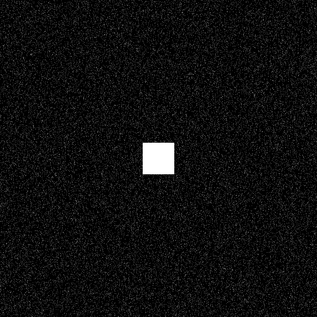
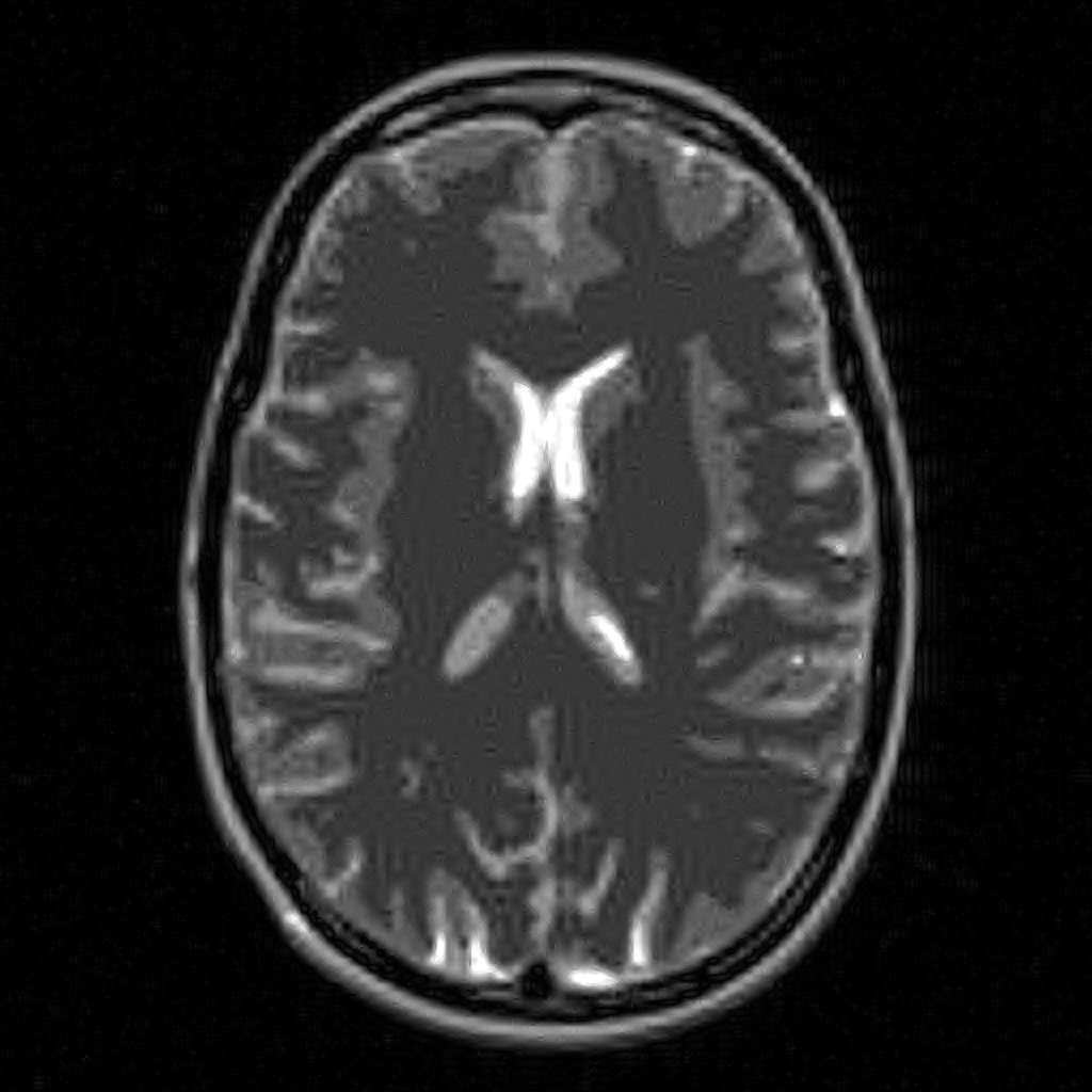
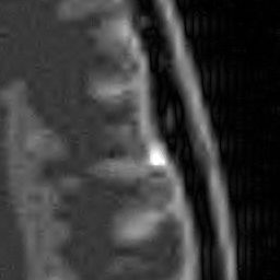
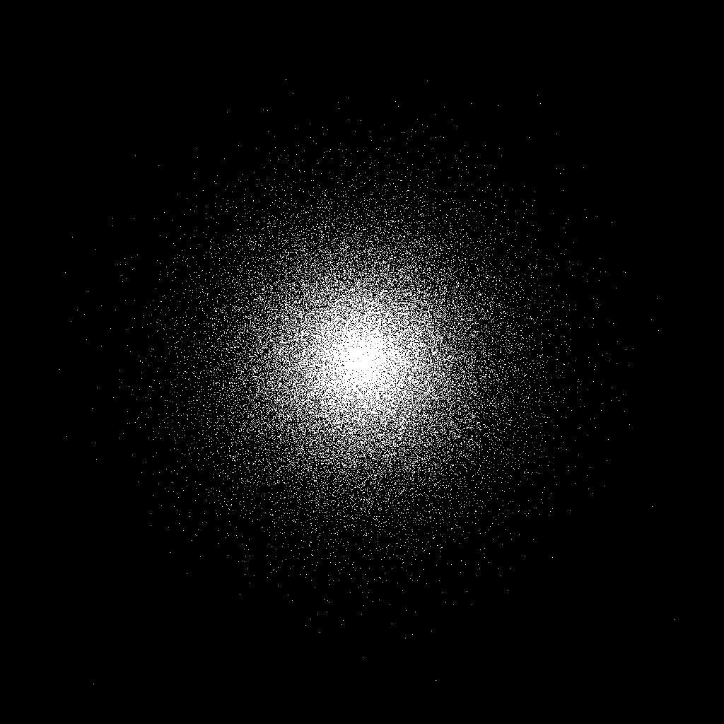
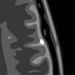
Figure 1: CS reconstruction from Fourier samples using wavelets. The subsampling strategy is displayed in the left column. Top: the uniform random subsampling strategy proposed by standard CS theory. Middle: two-level subsampling scheme (full sampling in the centre, uniform random subsampling outside). Bottom: Multi-level random subsampling strategy (see §4). The first scheme leads to poor reconstructions due to the high coherence. The latter two strategies exploit the asymptotic incoherence and asymptotic sparsity to obtain superior reconstructions.

We conclude the paper with a discussion of three particular consequences that arise from this new theory. First, in asymptotically sparse and asymptotically incoherent applications, the optimal sampling strategy will always depends on the signal structure. In particular, there can be no optimal sampling strategy for all sparse signals. Second, the well-known Restricted Isometry Property (RIP), although a popular tool in CS theory, is not witnessed in such applications. Hence, any RIP-based CS theory does not adequately explain the types of reconstruction results witnessed in practice.

Our third and final conclusion is that the success of compressed sensing is resolution dependent. At low resolutions, there is neither sufficient sparsity nor sufficient incoherence to give rise to high-quality reconstructions via CS. However, as the resolution increases, substantially better reconstructions become possible. In particular, CS with the appropriate subsampling strategy allows one to recover the fine details of images in a way that is not possible with conventional reconstruction strategies.

1.3 Relation to previous work

Generalized sampling was first introduced by Adcock & Hansen in a series of papers [BAACHSampTA, BAACHShannon, BAACHAccRecov]. An extension to sampling and reconstructing in different Hilbert spaces was considered in [AdcockHansenSpecData], and in [BAACHOptimality] the questions of sharp bounds and optimality of the reconstruction were considered. The particular case of GS for Fourier samples and wavelets was considered in [AHPWavelet]. §2 is based mainly on these papers. The extension of GS to inverse and ill-posed problems was presented in [AHHTillposed]. In §3 of this paper we improve the estimates given in [AHHTillposed] by using the geometric approach of [BAACHOptimality].

In [BAACHGSCS] a first theory of infinite-dimensional CS was presented, using ideas from generalized sampling. This was further developed in [AHPRBreaking] where the new principles asymptotic sparsity, asymptotic incoherence and multilevel random subsampling were introduced. §4 of this paper is based mainly on these works.

2 Generalized sampling – stable recovery in arbitrary frames

2.1 The abstract reconstruction problem

Let us first formally define the reconstruction problem we shall consider in this section. Suppose that $\{\psi_{j}\}_{j\in\mathbb{N}}$ is a collection of elements of a separable Hilbert space $\mathrm{H}$ (over $\mathbb{C}$) that forms a frame for a closed subspace $\mathrm{S}$ of $\mathrm{H}$ (the sampling space). In other words, $\mathrm{span}\{\psi_{j}\}_{j\in\mathbb{N}}$ is dense in $\mathrm{S}$ and there exist constants $c_{1},c_{2}>0$ such that

$$c_{1}\|f\|^{2}\leq\sum_{j\in\mathbb{N}}|\langle f,\psi_{j}\rangle|^{2}\leq c_{2}\|f\|^{2},\quad\forall f\in\mathrm{S},$$ (2.1)

where $\langle\cdot,\cdot\rangle$ and ${\left\|\cdot\right\|}$ are the inner product and norm on $\mathrm{H}$ respectively [christensen2003introduction]. We refer to $c_{1}$ and $c_{2}$ as the frame constants for $\{\psi_{j}\}_{j\in\mathbb{N}}$. Let $\{\varphi_{j}\}_{j\in\mathbb{N}}$ be a collection of reconstruction elements that form a frame for a closed subspace $\mathrm{T}$ (the reconstruction space), with frame constants $d_{1},d_{2}>0$:

$$d_{1}\|f\|^{2}\leq\sum_{j\in\mathbb{N}}|\langle f,\varphi_{j}\rangle|^{2}\leq d_{2}\|f\|^{2},\quad\forall f\in\mathrm{T}.$$ (2.2)

Finally, let $f\in\mathrm{H}$ be a given element we wish to recover, and assume that we have access to the samples

$$\hat{f}_{j}=\langle f,\psi_{j}\rangle,\quad j\in\mathbb{N}.$$ (2.3)

Note that the infinite vector $\hat{f}=\{\hat{f}_{j}\}_{j\in\mathbb{N}}\in\ell^{2}(\mathbb{N})$. Ignoring for the moment the issue of truncation – namely, that in practice we only have access to the first $N$ measurements – the abstract reconstruction problem can now be stated as follows:

Problem 2.1 (Infinite-dimensional reconstruction problem).

Given $\hat{f}=\{\hat{f}_{j}\}_{j\in\mathbb{N}}$, find a reconstruction $\tilde{f}$ of $f$ from the subspace $\mathrm{T}$.

As mentioned in §1, an importance instance of this problem is when the measurements arise as Fourier samples. In this case the sampling frame $\{\psi_{j}\}_{j\in\mathbb{N}}$ is a frame of complex exponentials. Typically, the reconstruction system $\{\varphi_{j}\}_{j\in\mathbb{N}}$ is taken to be a wavelet frame or basis, although other choices, such as orthogonal polynomials, may also be considered.

2.2 Stability and quasi-optimality

A reconstruction, in other words, a mapping $F:f\mapsto\tilde{f}\in\mathrm{T}$ based on the samples $\{\hat{f}_{j}\}_{j\in\mathbb{N}}$, ought to possess two important properties. The first of these is so-called quasi-optimality:

Definition 2.2.

Let $F$ be an operator on $\mathrm{H}_{0}$, where $\mathrm{H}_{0}$ is a closed subspace of $\mathrm{H}$, with range $\mathrm{T}$. The quasi-optimality constant of $\mu=\mu(F)>0$ is the least number such that

$$\|f-F(f)\|\leq\mu\|f-\mathcal{P}_{\mathrm{T}}f\|,\quad\forall f\in\mathrm{H}_{0},$$

where $\mathcal{P}_{\mathrm{T}}:\mathrm{H}\rightarrow\mathrm{T}$ is the orthogonal projection onto $\mathrm{T}$. If no such constant exists, we write $\mu=\infty$. We say that $F$ is quasi-optimal if $\mu(F)$ is small.

Since $\mathcal{P}_{\mathrm{T}}f$ is the best, i.e. energy-minimizing, approximation to $f$ from the reconstruction space $\mathrm{T}$, quasi-optimality states that the error committed by $\tilde{f}$ is within a small and constant factor of that of the best approximation. The need for quasi-optimality arises from the fact that typical images and signals are known to be well represented in certain bases and frames, e.g. wavelets or, in the case of smooth signals or images, polynomials [unser2000sampling]. In other words, the error $\|f-\mathcal{P}_{\mathrm{T}}f\|$ is small. It is therefore important that, when reconstructing $f$ in the corresponding subspace $\mathrm{T}$ from its measurements $\{\hat{f}_{j}\}_{j\in\mathbb{N}}$, the constant $\mu\ll\infty$. Otherwise, the beneficial property of $\mathrm{T}$ for the signal $f$ may be lost when passing to the reconstruction $\tilde{f}$.

The second important consideration is that of stability, which we quantify via the condition number:

Definition 2.3.

Let $\mathrm{H}_{0}$ be a closed subspace of $\mathrm{H}$ and suppose that $F:\mathrm{H}_{0}\rightarrow\mathrm{H}$ is a mapping such that, for each $f\in\mathrm{H}_{0}$, $F(f)$ depends only on the vector of samples $\hat{f}\in\ell^{2}(\mathbb{N})$. The (absolute) condition number $\kappa=\kappa(F)$ is given by

$$\kappa=\sup_{f\in\mathrm{H}_{0}}\lim_{\epsilon\rightarrow 0^{+}}\sup_{\begin{subarray}{c}g\in\mathrm{H}_{0}\\ 0<\|\hat{g}\|_{\ell^{2}}\leq\epsilon\end{subarray}}\left\{\frac{\|F(f+g)-F(f)\|}{\|\hat{g}\|_{\ell^{2}}}\right\}.$$ (2.4)

We say that $F$ is well-conditioned if $\kappa$ is small. Otherwise it is ill-conditioned.

A well-conditioned mapping $F$ is robust towards perturbations such as noise, and therefore this property is vital from a practical perspective.

We note that the condition number (2.4) does not assume linearity of $F$. If this is the case, then one has the much simpler form

$$\kappa(F)=\sup_{\begin{subarray}{c}f\in\mathrm{H}_{0}\\ \hat{f}\neq 0\end{subarray}}\left\{\frac{\|F(f)\|}{\|\hat{f}\|}\right\}.$$

We also remark that (2.4) is the absolute condition number, as opposed to the somewhat more standard relative condition number [TrefethenBau]. This is primarily for simplicity in the presentation: under some assumptions, it is possible to adapt the results we prove later in this paper for the latter.

We are now in a position to introduce the notion of a reconstruction constant for a mapping $F$:

Definition 2.4.

Let $F$ be as in Definition 2.3, and let $\mu(F)$ and $\kappa(F)$ be its quasi-optimality constant and condition number respectively. The reconstruction constant $C=C(F)$ is defined by $C(F)=\max\left\{\kappa(F),\mu(F)\right\}$. If $F$ is not quasi-optimal or if $\kappa(F)$ is not defined, then we set $C(F)=\infty$.

2.3 The computational reconstruction problem

In practice we do not have access to the infinite vector of samples $\hat{f}$. Thus in this section we shall primarily address the computation reconstruction problem: namely, the question of recovery of $f$ from its first $N$ measurements $\hat{f}_{1},\ldots,\hat{f}_{N}$. Since we only have access to these samples, it is natural to consider finite-dimensional subspaces of $\mathrm{T}$. In particular, we shall let $\{\mathrm{T}_{N}\}_{N\in\mathbb{N}}$ be a sequence of subspaces

$$\mathrm{T}_{N}\subseteq\mathrm{T},\qquad\dim(\mathrm{T}_{N})<\infty,\qquad\forall N\in\mathbb{N},$$ (2.5)

satisfying

$$\mathcal{P}_{\mathrm{T}_{N}}\rightarrow\mathcal{P}_{\mathrm{T}},\quad N\rightarrow\infty,$$ (2.6)

strongly on $\mathrm{H}$. In other words, $\{\mathrm{T}_{N}\}_{N\in\mathbb{N}}$ forms a sequence of finite-dimensional approximations to $\mathrm{T}$. Strictly, speaking, the second assumption is not necessary. However, it is natural so as to ensure a convergent approximation. Note also that, since $\{\varphi_{j}\}_{j\in\mathbb{N}}$ forms a frame $\mathrm{T}$, one usually defines $\mathrm{T}_{N}$ by

$$\mathrm{T}_{N}=\mathrm{span}\{\varphi_{j}\}_{j\in I_{N}},\quad\forall N\in\mathbb{N},$$ (2.7)

where the index sets $I_{1}\subseteq I_{2}\subseteq\ldots$ satisfy $\cup_{N\in\mathbb{N}}I_{N}=\mathbb{N}$.

We can now formulate the computational reconstruction problem:

Problem 2.5 (Computational reconstruction problem).

Given the samples $\hat{f}_{1},\ldots,\hat{f}_{N}$, compute a reconstruction to $f$ from the subspace $\mathrm{T}_{N}$.

When considering methods, i.e. mappings $F_{N}$, for this problem, it is desirable that the reconstruction constants $C(F_{N})$ should not grow rapidly with $N$. If this is not the case, then increasing the number of measurements could, for example, lead to a worse approximation and increased sensitivity to noise. Examples of this are discussed in §2.7. To avoid this scenario, we now make the following definition:

Definition 2.6.

For each $N\in\mathbb{N}$, let $F_{N}$ be such that, for each $f$, $F_{N}(f)$ depends only on the samples $\hat{f}^{[N]}=\{\hat{f}_{1},\ldots,\hat{f}_{N}\}$. We say that the reconstruction scheme $\{F_{N}\}_{N\in\mathbb{N}}$ is numerically stable and quasi-optimal if

$$C^{*}:=\sup_{N\in\mathbb{N}}C(F_{N})<\infty,$$

where $C(F_{N})$ is the reconstruction constant of $F_{N}$. We refer to the constant $C^{*}$ as the reconstruction constant of the reconstruction scheme $\{F_{N}\}_{N\in\mathbb{N}}$.

This definition incorporates the issue of stable approximation into a sequence of reconstruction schemes. Although in practice one only has access to a finite number of samples, it is natural to consider the behaviour of $F_{N}$ as $N$ – the number of samples – increases. Ideally, we want $F_{N}(f)$ to converge to $f$ at the same rate as $\mathcal{P}_{\mathrm{T}_{N}}f$, so that the beneficial approximation properties of the subspaces $\{\mathrm{T}_{N}\}_{N\in\mathbb{N}}$, i.e. the convergence of the projections $\mathcal{P}_{\mathrm{T}_{N}}f$, are not lost when passing to the reconstruction $F_{N}(f)$.

Later in this section we shall show that GS provides such a sequence of mapping $F_{N}$. Moreover, it leads to near-optimal reconstruction constants $C^{*}$. However, we first discuss another commonly used technique for this problem; so-called consistent reconstructions.

2.4 Consistent reconstructions

Consistent reconstructions (or consistent sampling) were introduced by Unser & Aldroubi [unser1994general, unserzerubia] as a simple and intuitive solution to Problem 2.1 and 2.5. They were later generalized significantly by Eldar et al.  [EldarRobConsistSamp, eldar2003FAA, eldar2003sampling, eldar2005general].

Let us first consider Problem 2.1. The consistent reconstruction arises by solving the so-called consistency conditions. Specifically, we let $\tilde{f}\in\mathrm{T}$ (whenever it exists uniquely) be the solution of

$$\langle\tilde{f},\psi_{j}\rangle=\langle f,\psi_{j}\rangle,\quad j=1,2,\ldots,\qquad\tilde{f}\in\mathrm{T}.$$ (2.8)

Note that consistency means that the samples of $\tilde{f}$ agree with those of $f$, which is intuitive from an engineering perspective since it stipulates that the reconstructed signal interpolates the available data. Correspondingly, we say that $\tilde{f}$ is a consistent reconstruction of $f$, and refer to the corresponding operator $F:f\mapsto\tilde{f}$, whenever defined, as consistent sampling.

In §2.6 we shall recap the standard the consistent reconstruction (2.8). In particular, we show that it possesses a near-optimal reconstruction constant, and therefore does indeed solve Problem 2.1.

Now consider the computational reconstruction problem, Problem 2.5. In this case, the corresponding consistent reconstruction [eldar2003FAA, eldar2003sampling, EldarMinimax, UnserHirabayashiConsist, unser2000sampling] is given as the solution of

$$\langle\tilde{f}_{N,N},\psi_{j}\rangle=\langle f,\psi_{j}\rangle,\quad j=1,\ldots,N,\qquad\tilde{f}_{N,N}\in\mathrm{T}_{N},$$ (2.9)

(the use of the double index in $\tilde{f}_{N,N}$ is for agreement with subsequent notation). Whilst this reconstruction retains the same intuitive notion of interpolating the available data, in §2.7 we shall show that in general the reconstruction $F_{N,N}$, if it exists (which is not guaranteed), can possess an arbitrarily large constants $C(F_{N,N})$. Hence consistent sampling when applied to Problem 2.5 can be both unstable and divergent. Generalized sampling, which we introduce in §2.9, overcomes these problems and leads to a stable, quasi-optimal reconstruction.

Before doing this, let us briefly note one property of consistent sampling. Namely, the reconstructions given by (2.8) and (2.9) are perfect for the subspaces $\mathrm{T}$ and $\mathrm{T}_{N}$ respectively. This means that $F(f)=f$ whenever $f\in\mathrm{T}$ for the former, and $F_{N,N}(f)=f$ whenever $f\in\mathrm{T}_{N}$ in the case of the latter (provided $F_{N,N}(f)$ exists uniquely).

2.5 Geometry of Hilbert spaces

In the next section we provide analysis of consistent sampling. For this, it is first useful to introduce some standard geometry of Hilbert spaces.

Definition 2.7.

Let $\mathrm{U}$ and $\mathrm{V}$ be closed subspaces of a Hilbert space $\mathrm{H}$ and let $\mathcal{P}_{\mathrm{V}}:\mathrm{H}\rightarrow\mathrm{V}$ be the orthogonal projection onto $\mathrm{V}$. The subspace angle $\theta=\theta_{\mathrm{U}\mathrm{V}}\in[0,\frac{\pi}{2}]$ between $\mathrm{U}$ and $\mathrm{V}$ is given by

$$\cos(\theta_{\mathrm{U}\mathrm{V}})=\inf_{\begin{subarray}{c}u\in\mathrm{U}\\ \|u\|=1\end{subarray}}\|\mathcal{P}_{V}u\|.$$ (2.10)

Note that there are a number of different ways to define the angle between subspaces [steinberg2000oblique, Tang1999Oblique]. However, (2.10) is the most convenient for our purposes. We shall also make use of the following equivalent expression for $\cos\left(\theta_{\mathrm{U}\mathrm{V}}\right)$:

$$\cos\left(\theta_{\mathrm{U}\mathrm{V}}\right)=\inf_{\begin{subarray}{c}u\in\mathrm{U}\\ \|u\|=1\end{subarray}}\sup_{\begin{subarray}{c}v\in\mathrm{V}\\ \|v\|=1\end{subarray}}\left|\langle u,v\rangle\right|.$$ (2.11)

Since we are interested in subspaces for which the cosine of the associated angle is nonzero, the following lemma will prove useful:

Lemma 2.8.

Let $\mathrm{U}$ and $\mathrm{V}$ be closed subspaces of a Hilbert space $\mathrm{H}$. Then $\cos\left(\theta_{\mathrm{U}\mathrm{V}^{\perp}}\right)>0$ if and only if $\mathrm{U}\cap\mathrm{V}=\{0\}$ and $\mathrm{U}+\mathrm{V}$ is closed $\mathrm{H}$.

Proof.

See [Tang1999Oblique, Thm. 2.1]. ∎

We now make the following definition:

Definition 2.9.

Let $\mathrm{U}$ and $\mathrm{V}$ be closed subspaces of a Hilbert space $\mathrm{H}$. Then $\mathrm{U}$ and $\mathrm{V}$ satisfy the subspace condition if $\cos\left(\theta_{\mathrm{U}\mathrm{V}^{\perp}}\right)>0$, or equivalently, if $\mathrm{U}\cap\mathrm{V}=\{0\}$ and $\mathrm{U}+\mathrm{V}$ is closed in $\mathrm{H}$.

Subspaces $\mathrm{U}$ and $\mathrm{V}$ satisfying this condition give a decomposition $\mathrm{U}\oplus\mathrm{V}=\mathrm{H}_{0}$ of a closed subspace $\mathrm{H}_{0}$ of $\mathrm{H}$. Equivalently, this ensures the existence of a projection of $\mathrm{H}_{0}$ with range $\mathrm{U}$ and kernel $\mathrm{V}$. We refer to such a projection as an oblique projection and denote it by $\mathcal{P}_{\mathrm{U}\mathrm{V}}$. Note that $\mathcal{P}_{\mathrm{U}\mathrm{V}}$ will not, in general, be defined over the whole of $\mathrm{H}$. However, this is true whenever $\mathrm{V}=\mathrm{U}^{\perp}$, for example, and in this case $\mathcal{P}_{\mathrm{U}\mathrm{V}}$ coincides with the orthogonal projection, which for succinctness we denote by $\mathcal{P}_{\mathrm{U}}$.

We shall also require the following results on oblique projections (see [BuckholtzIdempotents, SzyldOblProj]):

Theorem 2.10.

Let $\mathrm{U}$ and $\mathrm{V}$ be closed subspaces of $\mathrm{H}$ with $\mathrm{U}\oplus\mathrm{V}=\mathrm{H}$. Then

$$\|\mathcal{P}_{\mathrm{U}\mathrm{V}}\|=\|\mathcal{I}-\mathcal{P}_{\mathrm{U}\mathrm{V}}\|=\sec\left(\theta_{\mathrm{U}\mathrm{V}^{\perp}}\right),$$

where ${\left\|\cdot\right\|}$ is the standard norm on the space of bounded operators on $\mathrm{H}$.

Corollary 2.11.

Suppose that $\mathrm{U}$ and $\mathrm{V}$ are closed subspaces of $\mathrm{H}$ satisfying the subspace condition, and let $\mathcal{W}_{\mathrm{U}\mathrm{V}}:\mathrm{H}_{0}\rightarrow\mathrm{U}$ be the oblique projection with range $\mathrm{U}$ and kernel $\mathrm{V}$, where $\mathrm{H}_{0}=\mathrm{U}\oplus\mathrm{V}$. Then

$$\|\mathcal{P}_{\mathrm{U}\mathrm{V}}f\|\leq\sec\left(\theta_{\mathrm{U}\mathrm{V}^{\perp}}\right)\|f\|,\quad\forall f\in\mathrm{H}_{0},$$ (2.12)

and if $\mathcal{P}_{\mathrm{U}}:\mathrm{H}\rightarrow\mathrm{U}$ is the orthogonal projection,

$$\|f-\mathcal{P}_{\mathrm{U}}f\|\leq\|f-\mathcal{P}_{\mathrm{U}\mathrm{V}}f\|\leq\sec\left(\theta_{\mathrm{U}\mathrm{V}^{\perp}}\right)\|f-\mathcal{P}_{\mathrm{U}}f\|,\quad\forall f\in\mathrm{H}_{0}.$$ (2.13)

Moreover, the upper bounds in (2.12) and (2.13) are sharp.

Proof.

The sharp bound (2.12) is due to Theorem 2.10. For (2.13) we first note that $(\mathcal{I}-\mathcal{P}_{\mathrm{U}\mathrm{V}})=(\mathcal{I}-\mathcal{P}_{\mathrm{U}\mathrm{V}})(\mathcal{I}-\mathcal{P}_{\mathrm{U}})$, since $\mathcal{P}_{\mathrm{U}\mathrm{V}}$ and $\mathcal{P}_{\mathrm{U}}$ are both projections onto $\mathrm{U}$. Hence, by Theorem 2.10,

$$\|f-\mathcal{P}_{\mathrm{U}\mathrm{V}}f\|=\|(\mathcal{I}-\mathcal{P}_{\mathrm{U}\mathrm{V}})(\mathcal{I}-\mathcal{P}_{\mathrm{U}})f\|\leq\sec\left(\theta_{\mathrm{U}\mathrm{V}^{\perp}}\right)\|f-\mathcal{P}_{\mathrm{U}}f\|,$$

with sharp bound. ∎

• Although arbitrary subspaces $\mathrm{U}$ and $\mathrm{V}$ need not obey the subspace condition, this is often the case in practice. For example, if $\mathrm{U}\subseteq\mathrm{V}^{\perp}$ then $\cos\left(\theta_{\mathrm{U}\mathrm{V}^{\perp}}\right)=1$ by (2.11).

To complete this section, we present the following lemma which will be useful in what follows:

Lemma 2.12.

Let $\mathrm{U}$ and $\mathrm{V}$ be closed subspaces of $\mathrm{H}$ satisfying the subspace condition. Suppose also that $\dim(\mathrm{U})=\dim(\mathrm{V}^{\perp})=n<\infty$. Then $\mathrm{U}\oplus\mathrm{V}=\mathrm{H}$.

Proof.

Note that $\mathrm{U}\oplus\mathrm{V}=\mathrm{H}$ if and only if $\cos\left(\theta_{\mathrm{U}\mathrm{V}^{\perp}}\right)$ and $\cos\left(\theta_{\mathrm{V}^{\perp}\mathrm{U}}\right)$ are both positive [Tang1999Oblique, Thm. 2.3]. Since $\cos\left(\theta_{\mathrm{U}\mathrm{V}^{\perp}}\right)>0$ by assumption, it remains to show that $\cos\left(\theta_{\mathrm{V}^{\perp}\mathrm{U}}\right)>0$. Consider the mapping $\mathcal{P}_{\mathrm{V}^{\perp}}\big{|}_{\mathrm{U}}:\mathrm{U}\rightarrow\mathrm{V}^{\perp}$. We claim that this mapping is invertible. Since $\mathrm{U}$ and $\mathrm{V}^{\perp}$ have the same dimension it suffices to show that $\mathcal{P}_{\mathrm{V}^{\perp}}\big{|}_{\mathrm{U}}$ has trivial kernel. However, the existence of a nonzero $u\in\mathrm{U}$ with $\mathcal{P}_{\mathrm{V}^{\perp}}u=0$ implies that $\cos\left(\theta_{\mathrm{U}\mathrm{V}^{\perp}}\right)=0$; a contradiction. Thus $\mathcal{P}_{\mathrm{V}^{\perp}}\big{|}_{\mathrm{U}}$ is invertible, and in particular, it has range $\mathrm{V}^{\perp}$. Now consider $\cos\left(\theta_{\mathrm{V}^{\perp}\mathrm{U}}\right)$. By (2.11) and this result,

$$\cos\left(\theta_{\mathrm{V}^{\perp}\mathrm{U}}\right) =\inf_{\begin{subarray}{c}w\in\mathrm{V}^{\perp}\\ w\neq 0\end{subarray}}\sup_{\begin{subarray}{c}u\in\mathrm{U}\\ u\neq 0\end{subarray}}\frac{\left|\langle w,u\rangle\right|}{\|w\|\|u\|}=\inf_{\begin{subarray}{c}u^{\prime}\in\mathrm{U}\\ u^{\prime}\neq 0\end{subarray}}\sup_{\begin{subarray}{c}u\in\mathrm{U}\\ u\neq 0\end{subarray}}\frac{\left|\langle\mathcal{P}_{\mathrm{V}^{\perp}}u^{\prime},u\rangle\right|}{\|\mathcal{P}_{\mathrm{V}^{\perp}}u^{\prime}\|\|u\|}\geq\inf_{\begin{subarray}{c}u^{\prime}\in\mathrm{U}\\ u^{\prime}\neq 0\end{subarray}}\frac{\|\mathcal{P}_{\mathrm{V}^{\perp}}u^{\prime}\|}{\|u^{\prime}\|}=\cos\left(\theta_{\mathrm{U}\mathrm{V}^{\perp}}\right)>0.$$

This completes the proof. ∎

The following lemma will also be useful:

Lemma 2.13.

Let $\mathrm{U}$ and $\mathrm{V}$ be closed subspaces of $\mathrm{H}$ satisfying the subspace condition. Let $f\in\mathrm{H}_{0}:=\mathrm{U}\oplus\mathrm{V}$ and consider the following variational problem:

find $$\tilde{f}\in\mathrm{U} \langle\tilde{f},w\rangle=\langle f,w\rangle \forall w\in\mathrm{V}^{\perp}$$ satisfying , . (2.14)

Then this problem has a unique solution $\tilde{f}$ and it coincides with $\mathcal{P}_{\mathrm{U}\mathrm{V}}f$.

Proof.

Since $\mathrm{U}$ and $\mathrm{V}$ satisfy the subspace condition, $\mathcal{P}_{\mathrm{U}\mathrm{V}}$ exists uniquely. Note that $\mathcal{P}_{\mathrm{U}\mathrm{V}}f$ is a solution of the variational problem. Hence it remains to show that the variational problem has a unique solution. Suppose not. Then there exists a nonzero $\tilde{f}\in\mathrm{U}$ with $\langle\tilde{f},w\rangle=0$, $\forall w\in\mathrm{V}^{\perp}$. Hence $\tilde{f}\in\mathrm{U}\cap\mathrm{V}$, which contradicts the fact that $\mathrm{U}$ and $\mathrm{V}$ satisfy the subspace condition. ∎

2.6 The reconstruction constant of consistent sampling

We now analyze the reconstruction constant of consistent sampling for Problems 2.1 and 2.5. The usual approach [unser1994general, eldar2005general] for doing this is based on associating the corresponding mappings with appropriate oblique projections, and then applying the results given in the previous section.

2.6.1 The case of Problem 2.1

Our main results are as follows:

Theorem 2.14.

Suppose that $\mathrm{T}$ and $\mathrm{S}^{\perp}$ satisfy the subspace condition. If $f\in\mathrm{H}_{0}:=\mathrm{T}\oplus\mathrm{S}^{\perp}$, then there exists a unique $\tilde{f}\in\mathrm{T}$ satisfying (2.8). In particular, the consistent reconstruction $F:\mathrm{H}_{0}\rightarrow\mathrm{T}$, $f\mapsto\tilde{f}$ is well-defined. Moreover, it coincides with the oblique projection $\mathcal{P}_{\mathrm{T}\mathrm{S}^{\perp}}$ with range $\mathrm{T}$ and kernel $\mathrm{S}^{\perp}$.

Proof.

By linearity, (2.8) is equivalent to (2.14) with $\mathrm{U}=\mathrm{T}$ and $\mathrm{V}=\mathrm{S}^{\perp}$. Since $\mathrm{T}$ and $\mathrm{S}^{\perp}$ satisfy the subspace condition, Lemma 2.13 demonstrates that the consistent reconstruction $F$ is well-defined on $\mathrm{H}_{0}$ and coincides with the oblique projection $\mathcal{P}_{\mathrm{T}\mathrm{S}^{\perp}}$. ∎

Corollary 2.15.

Suppose that $\mathrm{T}$ and $\mathrm{S}^{\perp}$ satisfy the subspace condition and let $F:\mathrm{H}_{0}:=\mathrm{T}\oplus\mathrm{S}^{\perp}\rightarrow\mathrm{T}$, $f\mapsto\tilde{f}$ be the consistent reconstruction (2.8). Then the quasi-optimality constant and condition number satisfy

$$\mu(F)=\sec\left(\theta_{\mathrm{T}\mathrm{S}}\right),\qquad\frac{\sec\left(\theta_{\mathrm{T}\mathrm{S}}\right)}{\sqrt{c_{2}}}\leq\kappa(F)\leq\frac{\sec\left(\theta_{\mathrm{T}\mathrm{S}}\right)}{\sqrt{c_{1}}},$$

and therefore

$$\sec\left(\theta_{\mathrm{T}\mathrm{S}}\right)\max\{1,1/\sqrt{c_{2}}\}\leq C(F)\leq\sec\left(\theta_{\mathrm{T}\mathrm{S}}\right)\max\{1,1/\sqrt{c_{1}}\}.$$

To prove this corollary, it is necessary to first recall several basic facts about frames [christensen2003introduction]. Given the sampling frame $\{\psi_{j}\}_{j\in\mathbb{N}}$ for the subspace $\mathrm{S}$, we define the synthesis operator $S:\ell^{2}(\mathbb{N})\rightarrow\mathrm{H}$ by

$$S\alpha=\sum_{j\in\mathbb{N}}\alpha_{j}\psi_{j},\quad\alpha=\{\alpha_{j}\}_{j\in\mathbb{N}}\in\ell^{2}(\mathbb{N}).$$

Its adjoint, the analysis operator, is defined by

$$S^{*}f=\hat{f}=\{\langle f,\psi_{j}\rangle\}_{j\in\mathbb{N}},\quad f\in\mathrm{H}.$$

The resulting composition $\mathcal{S}=SS^{*}:\mathrm{H}\rightarrow\mathrm{H}$, given by

$$\mathcal{S}f=\sum_{j\in\mathbb{N}}\langle f,\psi_{j}\rangle\psi_{j},\quad\forall f\in\mathrm{H},$$ (2.15)

is well-defined, linear, self-adjoint and bounded. Moreover, the restriction $\mathcal{S}|_{\mathrm{S}}:\mathrm{S}\rightarrow\mathrm{S}$ is positive and invertible with $c_{1}\mathcal{I}|_{\mathrm{S}}\leq\mathcal{S}|_{\mathrm{S}}\leq c_{2}\mathcal{I}|_{\mathrm{S}}$, where $c_{1},c_{2}$ are the frame constants appearing in (2.1).

We now require the following lemma:

Lemma 2.16.

Suppose that $\mathrm{T}$ and $\mathrm{S}^{\perp}$ satisfy the subspace condition, and let $\mathcal{S}$ be given by (2.15). Then

$$c_{1}\cos^{2}(\theta_{\mathrm{T}\mathrm{S}})\hskip 2.84526pt\mathcal{I}|_{\mathrm{T}}\leq\mathcal{S}|_{\mathrm{T}}\leq c_{2}\mathcal{I}|_{\mathrm{T}}.$$ (2.16)

Proof.

Let $f\in\mathrm{H}$ be arbitrary, and write $f=\mathcal{P}_{\mathrm{S}}f+\mathcal{P}_{\mathrm{S}^{\perp}}f$. Then

$$\langle\mathcal{S}f,f\rangle=\sum_{j\in\mathbb{N}}|\langle f,\psi_{j}\rangle|^{2}=\sum_{j\in\mathbb{N}}|\langle\mathcal{P}_{\mathrm{S}}f,\psi_{j}\rangle|^{2}=\langle\mathcal{S}\mathcal{P}_{\mathrm{S}}f,\mathcal{P}_{\mathrm{S}}f\rangle.$$ (2.17)

Suppose now that $\varphi\in\mathrm{T}$. Using (2.17) and the frame condition (2.1) we find that

$$c_{1}\|\mathcal{P}_{\mathrm{S}}\varphi\|^{2}\leq\langle\mathcal{S}\varphi,\varphi\rangle\leq c_{2}\|\mathcal{P}_{\mathrm{S}}\varphi\|^{2}\leq c_{2}\|\varphi\|^{2}.$$

To obtain (2.16) we now use the definition of the subspace angle $\theta_{\mathrm{T}\mathrm{S}}$. ∎

Proof of Corollary 2.15.

Since $\tilde{f}$ coincides with the oblique projection (Theorem 2.14), an application of Corollary (2.11) gives that

$$\|f-F(f)\|\leq\sec\left(\theta_{\mathrm{T}\mathrm{S}}\right)\|f-\mathcal{P}_{\mathrm{T}}f\|,\quad\forall f\in\mathrm{H}_{0},$$

and since this bound is sharp, we deduce that $\mu(F)=\sec\left(\theta_{\mathrm{T}\mathrm{S}}\right)$.

It remains to estimate $\kappa(F)$. Let $f\in\mathrm{H}_{0}$ be arbitrary and consider $\tilde{f}=F(f)\in\mathrm{T}$. We have

$$\|\hat{f}\|^{2}_{\ell^{2}}=\sum_{j\in\mathbb{N}}|\langle f,\psi_{j}\rangle|^{2}=\sum_{j\in\mathbb{N}}|\langle\tilde{f},\psi_{j}\rangle|^{2}=\langle\mathcal{S}\tilde{f},\tilde{f}\rangle.$$

Hence, by the previous lemma, $\|\hat{f}\|^{2}_{\ell^{2}}\geq c_{1}\cos^{2}(\theta_{\mathrm{T}\mathrm{S}})\|\tilde{f}\|^{2}$. Since $F$ is linear, this now gives

$$\kappa(F)=\sup_{\begin{subarray}{c}f\in\mathrm{H}_{0}\\ \hat{f}\neq 0\end{subarray}}\left\{\frac{\|F(f)\|}{\|\hat{f}\|_{\ell^{2}}}\right\}\leq\frac{\sec(\theta_{\mathrm{T}\mathrm{S}})}{\sqrt{c_{1}}}.$$

On the other hand, since the reconstruction $F$ is perfect for the subspace $\mathrm{T}$, and since $\hat{f}=0$ if and only if $f=0$ for $f\in\mathrm{T}$,

$$\kappa(F)\geq\sup_{\begin{subarray}{c}f\in\mathrm{T}\\ \hat{f}\neq 0\end{subarray}}\left\{\frac{\|f\|}{\|\hat{f}\|_{\ell^{2}}}\right\}=\sup_{\begin{subarray}{c}f\in\mathrm{T}\\ f\neq 0\end{subarray}}\left\{\frac{\|f\|}{\|\hat{f}\|_{\ell^{2}}}\right\}.$$

By (2.17), we have $\|\hat{f}\|^{2}_{\ell^{2}}\leq c_{2}\|\mathcal{P}_{\mathrm{S}}f\|^{2}$. Hence

$$\kappa(F)\geq\frac{1}{\sqrt{c_{2}}}\sup_{\begin{subarray}{c}f\in\mathrm{T}\\ f\neq 0\end{subarray}}\left\{\frac{\|f\|}{\|\mathcal{P}_{\mathrm{S}}f\|}\right\}=\frac{\sec(\theta_{\mathrm{T}\mathrm{S}})}{\sqrt{c_{2}}},$$

as required. ∎

2.6.2 The case of Problem 2.5

We now consider the computational reconstruction problem (Problem 2.5).

Theorem 2.17.

Let $\mathrm{S}_{N}=\mathrm{span}\{\psi_{1},\ldots,\psi_{N}\}$ and suppose that

$$\cos\left(\theta_{N,N}\right)>0,$$ (2.18)

where $\theta_{N,N}=\theta_{\mathrm{T}_{N}\mathrm{S}_{N}}$. Then, for each $f\in\mathrm{H}_{N}:=\mathrm{T}_{N}\oplus\mathrm{S}^{\perp}_{N}$ there exists a unique $\tilde{f}_{N,N}\in\mathrm{T}_{N}$ satisfying (2.9). In particular, the consistent reconstruction $F_{N,N}:\mathrm{H}_{N}\rightarrow\mathrm{T}_{N}$, $f\mapsto\tilde{f}_{N,N}$ is well-defined and coincides with the oblique projection $\mathcal{P}_{\mathrm{T}_{N}\mathrm{S}^{\perp}_{N}}$ with range $\mathrm{T}_{N}$ and kernel $\mathrm{S}^{\perp}_{N}$.

Proof.

This follows immediately from Lemma 2.13 with $\mathrm{U}=\mathrm{T}_{N}$ and $\mathrm{V}=\mathrm{S}^{\perp}_{N}$. ∎

Corollary 2.18.

Let $\theta_{N,N}$, $\mathrm{H}_{N}$ and $F_{N,N}$ be as in Theorem 2.17. Then the quasi-optimality constant and condition number satisfy

$$\mu(F_{N,N})=\sec\left(\theta_{N,N}\right),\qquad\kappa(F_{N,N})\geq\frac{\sec\left(\theta_{N,N}\right)}{\sqrt{c_{2}}},$$

and therefore

$$C(F_{N,N})\geq\max\left\{1,1/\sqrt{c_{2}}\right\}\sec\left(\theta_{N,N}\right).$$

Proof.

This follows immediately from Lemma 2.19 and Corollary 2.23. ∎

2.7 Failure of consistent sampling for Problem 2.5

Theorem 2.14 shows that consistent sampling provides a stable, quasi-optimal solution to Problem 2.1, provided $\cos\left(\theta_{\mathrm{T}\mathrm{S}}\right)\neq 0$, or in other words, whenever the spaces $\mathrm{T}$ and $\mathrm{S}$ are not perpendicular. According to Theorem 2.17, the same conclusion holds for Problem 2.5 if the subspace angles $\theta_{N,N}$ are bounded away from $\pi/2$. Unfortunately, there is no general guarantee that this will be the case. Moreover, as the following examples illustrate, it is typical for the quantities $\cos(\theta_{N,N})$ to behave wildly:

• Let $\mathrm{H}=\mathrm{L}^{2}(-1,1)$ and consider the orthonormal Fourier sampling basis:

  $$\psi_{j}(x)=\frac{1}{\sqrt{2}}\mathrm{e}^{\mathrm{i}j\pi x},\quad j\in\mathbb{Z}.$$

  Let $\mathrm{S}_{N}=\mathrm{span}\{\psi_{j}:j=-(N-1)/2,\ldots,(N-1)/2\}$ (we shall assume that $N$ is odd for convenience), and consider the reconstruction space $\mathrm{T}_{N}=\mathbb{P}_{N-1}$ of polynomials of degree less than $N$. Note that if $\{\varphi_{j}\}_{j\in\mathbb{N}}$ is the orthonormal basis of Legendre polynomials for $\mathrm{H}$, then $\mathrm{T}_{N}$ takes the form (2.7) with index set $I_{N}=\{1,\ldots,N\}$, i.e. $\mathrm{T}_{N}=\mathrm{span}\{\varphi_{1},\ldots,\varphi_{N}\}$.

  In [AdcockHansenShadrinStabilityFourier] it was proved that

  $$\cos(\theta_{N,N})\leq c^{-N},\quad\forall N,$$

  for some constant $c>1$, and therefore the reconstruction constant $C(F_{N,N})\geq c^{N}$ grows exponentially fast in $N$. This translates into both extreme instability and divergence of the reconstruction.

• Let $\mathrm{H}=\mathrm{L}^{2}(-1,1)$ and let $\psi_{j}$ and $\mathrm{S}_{N}$ be as in the previous example. Let $\{\varphi_{j}\}_{j\in\mathbb{N}}$ be the orthonormal basis of Haar wavelets on $[0,1]$, and set $\mathrm{T}_{N}=\mathrm{span}\left\{\varphi_{1},\ldots,\varphi_{N}\right\}$, i.e. the finite-dimensional subspace spanned by the first $N$ Haar wavelets. In [AHPWavelet] it was proved that, much as in the previous example, $\cos(\theta_{N,N})$ is exponentially small in $N$. Hence the same conclusions – namely, instability and divergence of the consistent reconstruction – hold.

  Note that this phenomenon is not isolated to Haar wavelets. One sees exactly the same type of behaviour for essentially all orthonormal bases of compactly supported wavelets. See [AHPWavelet].

As a particular consequence, these examples illustrate that boundedness of the infinite subspace angle $\theta_{\mathrm{T}\mathrm{S}}$ away from $\pi/2$ does not guarantee the same for the finite subspace angles $\theta_{N,N}$. Or equivalently, the spaces $\mathrm{T}_{N}$ and $\mathrm{S}_{N}$ can be near-perpendicular, even when $\mathrm{T}$ and $\mathrm{S}$ are not.

2.8 Linear systems and connections to finite sections of operators

It is interesting to reinterpret this failure of consistent reconstruction in terms of spectral properties of truncations of operators. This will be particularly useful in §3.

Let $\hat{f}=\{\hat{f}_{j}\}_{j\in\mathbb{N}}$ be the infinite vector of samples of $f$, and define the infinite matrix

$$A=\left(\begin{array}[]{ccc}\left<\varphi_{1},\psi_{1}\right>&\left<\varphi_{2},\psi_{1}\right>&\cdots\\ \left<\varphi_{1},\psi_{2}\right>&\left<\varphi_{2},\psi_{2}\right>&\cdots\\ \vdots&\vdots&\ddots\end{array}\right),$$ (2.19)

Since both the sampling and reconstruction systems are frames, the matrix $A$ can be viewed as a bounded operator on $\ell^{2}(\mathbb{N})$. Moreover, if $S$ and $T$ are the synthesis operators for $\{\psi_{j}\}^{\infty}_{j=1}$ and $\{\varphi_{j}\}^{\infty}_{j=1}$ respectively, then we may express $A$ as the product $S^{*}T$. It is readily seen that if the infinite-dimensional consistent reconstruction $\tilde{f}$ is expressed as

$$\tilde{f}=T\beta=\sum_{j\in\mathbb{N}}\beta_{j}\varphi_{j},$$

for some $\beta=\{\beta_{j}\}_{j\in\mathbb{N}}\in\ell^{2}(\mathbb{N})$, then $\beta$ satisfies the infinite linear system

$$A\beta=\hat{f}.$$ (2.20)

Now consider the computational consistent reconstruction (2.9), and suppose that, as in the previous examples, we let

$$\mathrm{T}_{N}=\mathrm{span}\{\varphi_{1},\ldots,\varphi_{N}\}.$$

If $\{e_{j}\}_{j\in\mathbb{N}}$ is the canonical basis for $\ell^{2}(\mathbb{N})$, let

$$P_{N}:\ell^{2}(\mathbb{N})\rightarrow\mathrm{span}\{e_{1},\ldots,e_{n}\},$$

be the orthogonal projection. If we now write the consistent reconstruction (2.9) as

$$\tilde{f}_{N,N}=T_{N}\beta^{[N,N]}=\sum^{N}_{j=1}\beta^{[N,N]}_{j}\varphi_{j},$$

then the vector $\beta^{[N,N]}\in P_{N}(\ell^{2}(\mathbb{N}))$ satisfies

$$A^{[N,N]}\beta^{[N,N]}=P_{N}\hat{f},\qquad A^{[N,N]}=P_{N}AP_{N}.$$ (2.21)

Note that this is just an $N\times N$ linear system for the vector $\beta^{[N,N]}$. Note also that $A^{[N,N]}=S^{*}_{N}T_{N}$, where $S_{N}$ and $T_{N}$ are the synthesis operators for the finite frame sequences $\{\psi_{1},\ldots,\psi_{N}\}$ and $\{\varphi_{1},\ldots,\varphi_{N}\}$ respectively, and therefore one may write

$$\tilde{f}_{N,N}=T_{N}\beta^{[N,N]}=T_{N}(S^{*}_{N}T_{N})^{-1}S^{*}_{N}f,$$ (2.22)

whenever $A^{[N,N]}$ is invertible.

This leads to an alternative viewpoint of the computational consistent reconstruction. In particular, we may consider (2.21) as a discretization of the infinite linear system (2.20). Moreover, since $P_{N}AP_{N}$ is the leading $N\times N$ submatrix of $A$, the discretization (2.21) is nothing more than an instance of the well-known finite section method for solving infinite linear systems applied to (2.20).

Suppose now for simplicity that both $\{\psi_{j}\}_{j\in\mathbb{N}}$ and $\{\varphi_{j}\}_{j\in\mathbb{N}}$ are orthonormal bases. Then one can show that $\cos(\theta_{N,N})$ and $\cos(\theta)$ coincide with the minimal singular values of the matrices $A^{[N,N]}$ and $A$ respectively (the latter quantity being precisely $1$ since $A$ is an isometry in this case). Hence, the fact that $\theta_{N,N}$ may behave wildly, even when $\theta$ is bounded away from $\pi/2$, demonstrates that the spectra of the finite sections $A^{[N,N]}$ poorly approximate the spectrum of $A$.

This question – namely, how well does a sequence of finite-rank operators approximate the spectrum of a given infinite-rank operator – is one of the most fundamental in the field of spectral theory. Within this field, finite sections have been studied extensively over the last several decades [bottcher1996, hansen2008, lindner2006]. Unfortunately there is no guarantee that they be well behaved.

To put this in a formal perspective, suppose for the moment that we approximate the operator $A$ with a sequence $A^{[N]}$ of finite-rank operators (which may or may not be finite sections), and instead of solving $A\beta=\hat{f}$, we solve $A^{[N]}\beta^{[N]}=\hat{f}^{[N]}$. For obvious reasons, it is vitally important that this sequence satisfies the three following conditions:

1. Invertibility: $A^{[N]}$ is invertible for all $n=1,2,\ldots$.

2. Stability: $\|(A^{[N]})^{-1}\|$ is uniformly bounded for all $N=1,2,\ldots$.

3. Convergence: the solutions $\beta^{[N]}\rightarrow\beta$ as $N\rightarrow\infty$.

Unfortunately, there is no guarantee that finite sections, and therefore the consistent reconstruction technique, possess any of these properties. In fact, one requires rather restrictive conditions on $A$, such as positive self-adjointness, for this to be the case. Typically operators of the form (2.19) are not self-adjoint, thereby making finite sections unsuitable in general for discretizing the system $A\beta=\hat{f}$.

Fortunately, these issues can be overcome by performing an alternative discretization of $A$. This leads to a sequence of operators that possess the properties (i)–(iii) above, and culminates in the GS technique. The key to doing this is to allow the number of samples $N$ and the number of index $M$ of the reconstruction subspace $\mathrm{T}_{M}$ to differ. When $N$ is sufficiently large for a given $M$, or equivalently, $M$ is sufficiently small for a given $N$, we obtain a finite-dimensional operator $A^{[N,M]}$ (which now depends on both $N$ and $M$) that inherits the spectral structure of its infinite-dimensional counterpart $A$. This ensures a stable, quasi-optimal reconstruction.

2.9 Generalized sampling

From now on, we shall assume that the subspaces $\mathrm{T}$ and $\mathrm{S}^{\perp}$ satisfy the subspace condition.

We now introduce generalized sampling. Let $\mathrm{S}_{N}=\mathrm{span}\{\psi_{1},\ldots,\psi_{N}\}$ and suppose that $\{\mathrm{T}_{M}\}_{M\in\mathbb{N}}$ is a sequence of subspaces obeying (2.5) and (2.6). We seek a reconstruction $\tilde{f}_{N,M}\in\mathrm{T}_{M}$ of $f$ from the $N$ samples $\hat{f}_{1},\ldots,\hat{f}_{N}$. Let $\mathcal{S}_{N}:\mathrm{H}\rightarrow\mathrm{S}_{N}$ be the finite rank operator given by

$$\mathcal{S}_{N}g=S_{N}S^{*}_{N}g=\sum^{N}_{j=1}\langle g,\psi_{j}\rangle\psi_{j}.$$

Note that the sequence of operators $\mathcal{S}_{N}$ converge strongly to $\mathcal{S}$ on $\mathrm{H}$ as $N\rightarrow\infty$, where $\mathcal{S}$ is given by (2.15), since $\{\psi_{j}\}_{j\in\mathbb{N}}$ is a frame [christensen2003introduction]. With this to hand, the approach originally proposed in [BAACHShannon] is to define $\tilde{f}_{N,M}\in\mathrm{T}_{M}$ as the solution of the equations

$$\langle\mathcal{S}_{N}\tilde{f}_{N,M},\varphi_{j}\rangle=\langle\mathcal{S}_{N}f,\varphi_{j}\rangle,\quad j=1,\ldots,M,\qquad\tilde{f}_{N,M}\in\mathrm{T}_{M}.$$ (2.23)

We refer to the mapping $F_{N,M}:f\mapsto\tilde{f}_{N,M}$, whenever defined, as generalized sampling (GS). Observe that $\mathcal{S}_{M}f$ is determined solely by the samples $\hat{f}_{1},\ldots\hat{f}_{M}$. Hence $F_{N,M}(f)$ is also determined only by these values.

In what follows it will be useful to note that (2.23) is equivalent to

$$\langle\tilde{f}_{N,M},\mathcal{S}_{N}\varphi_{j}\rangle=\langle f,\mathcal{S}_{N}\varphi_{j}\rangle,\quad j=1,\ldots,M,\qquad\tilde{f}_{N,M}\in\mathrm{T}_{M},$$ (2.24)

due to the self-adjointness of $\mathcal{S}_{N}$. An immediate consequence of this formulation is the following:

Lemma 2.19.

Suppose that $\cos(\theta_{N,N})>0$ and that $\dim(\mathrm{S}_{N})=\dim(\mathrm{T}_{N})$. Then when $M=N$ the GS reconstruction $\tilde{f}_{N,M}$ of $f\in\mathrm{H}$ defined by (2.23) is precisely the consistent reconstruction $\tilde{f}_{N,N}$ defined by (2.9).

Proof.

We first claim that $\mathcal{S}_{N}$ is a bijection from $\mathrm{T}_{N}$ to $\mathrm{S}_{N}$. Suppose that $\mathcal{S}_{N}\varphi=0$ for some $\varphi\in\mathrm{T}_{N}$. Then $0=\langle\mathcal{S}_{N}\varphi,\varphi\rangle=\sum^{N}_{j=1}|\langle\varphi,\psi_{j}\rangle|^{2}$ and therefore $\varphi\in\mathrm{S}^{\perp}_{N}$. Since $\varphi\in\mathrm{T}_{N}$, and $\mathrm{T}_{N}\cap\mathrm{S}^{\perp}_{N}=\{0\}$ by assumption, we have $\varphi=0$, as required.

By linearity, we now find that the conditions (2.24) are equivalent to (2.9). Since the consistent reconstruction $\tilde{f}_{n,n}$ satisfying (2.8) exists uniquely (Theorem 2.17), we obtain the result. ∎

We conclude that GS contains consistent sampling as a special case corresponding to $M=N$, which explains our use of the same notation for both. However, as mentioned above, the key to GS is to allow $N$ and $M$ to vary independently. As we prove in §2.11, doing so leads to a small reconstruction constant.

2.10 Generalized sampling and uneven sections of operators

Before this, let us first connect GS to the linear systems interpretation of §2.8. Let

$$\tilde{f}_{N,M}=T_{N}\beta^{[N,M]}=\sum^{M}_{j=1}\beta^{[N,M]}_{j}\varphi_{j},$$

for some vector $\beta^{[N,M]}\in P_{M}(\ell^{2}(\mathbb{N}))$. Then it is readily seen that (2.23) is equivalent to the linear system

$$(A^{[N,M]})^{*}A^{[N,M]}\beta^{[N,M]}=(A^{[N,M]})^{*}P_{N}\hat{f},\qquad A^{[N,M]}=P_{N}AP_{M}.$$ (2.25)

The matrix $A^{[N,M]}$ is the leading $N\times M$ submatrix of the infinite matrix $A$, and is commonly referred to as an uneven section of $A$. Uneven sections have recently gained prominence as effective alternatives to the finite section method for discretizing non-self adjoint operators [strohmer, Lindner2008]. In particular, in [hansen2011] they were employed to solve the long-standing computational spectral problem. Their success is due to the observation that, under a number of assumptions (which are always guaranteed for the problem we consider in this paper), we have

$$(A^{[N,M]})^{*}A^{[N,M]}=P_{M}A^{*}P_{N}AP_{M}\rightarrow P_{M}A^{*}AP_{M},\quad N\rightarrow\infty,$$

where $P_{M}A^{*}AP_{M}$ is the $M\times M$ finite section of the self-adjoint matrix $A^{*}A$. This guarantees properties (i)–(iii) listed in §2.8 for $A^{[N,M]}$, whenever $N$ is sufficiently large in comparison to $M$. In other words, whereas the finite section $P_{M}AP_{M}$ can possess wildly different spectral properties those of $A$, the uneven section $P_{N}AP_{M}$ is guaranteed to inherit those properties whenever $N$ is sufficiently large.

Note that finite (and uneven) sections have been extensively studied [bottcher1996, hansen2008, lindner2006], and there exists a well-developed theory of their properties involving $C^{*}$-algebras [hagen2001c]. However, these general results say little about the rate of convergence as $N\rightarrow\infty$, nor do they provide explicit constants. Yet, as we shall see next, the operator $A$ in this case is so structured that its uneven sections admit both explicit constants and estimates for the rate of convergence. Moreover, of great practical importance, such constants can also be numerically computed (see §2.12).

This aside, let us briefly not that the GS reconstruction, much as with the consistent reconstruction (2.22), can be reformulated in terms of synthesis and analysis operators. Indeed, the matrix $A^{[N,M]}$ is equivalent to $S^{*}_{N}T_{M}$, and therefore

$$\tilde{f}_{N,M}=T_{M}(T_{M}S_{N}S^{*}_{N}T_{M})^{-1}T^{*}_{M}S_{N}S^{*}_{N}f.$$ (2.26)

This formulation will be of use in §3.

2.11 Analysis of generalized sampling

Let us first define the subspace angle

$$\theta_{N,M}:=\theta_{\mathrm{T}_{M},\mathcal{S}_{N}(\mathrm{T}_{M})},\quad N,M\in\mathbb{N}.$$ (2.27)

Before stating our main results, we first require the following lemma:

Lemma 2.20.

Let $\theta_{N,M}$ be given by (2.27). Then

$$\lim_{N\rightarrow\infty}\theta_{N,M}=\theta_{\infty,M},$$

where $\theta_{\infty,M}=\theta_{\mathrm{T}_{M},\mathcal{S}(\mathrm{T}_{M})}$. In particular,

$$1\leq\lim_{N\rightarrow\infty}\sec\left(\theta_{N,M}\right)\leq\sqrt{\frac{c_{2}}{c_{1}}}\sec\left(\theta_{\mathrm{T}\mathrm{S}}\right).$$

Proof.

See [BAACHOptimality, Lem. 4.4]. ∎

This lemma illustrates that the subspace angle $\theta_{N,M}$ is well-behaved whenever $N$ is sufficiently large in comparison to $M$. Unlike the consistent reconstruction, which is based on the poorly-behaved angle $\theta_{N,N}$, this ensures stability and quasi-optimality of GS. We have:

Theorem 2.21.

Let $M\in\mathbb{N}$ and suppose that $N\geq N_{0}$, where $N_{0}$ is the least $N$ such that $\cos\left(\theta_{N,M}\right)>0$. Then, for each $f\in\mathrm{H}$, there exists a unique $\tilde{f}_{N,M}\in\mathrm{T}_{M}$ satisfying (2.23). Moreover, the mapping $F_{N,M}:f\mapsto\tilde{f}_{N,M}$ is precisely the oblique projection $\mathcal{P}_{\mathrm{T}_{M},(\mathcal{S}_{N}(\mathrm{T}_{M}))^{\perp}}$ with range $\mathrm{T}_{M}$ and kernel $(\mathcal{S}_{N}(\mathrm{T}_{M}))^{\perp}$.

Proof.

See [BAACHOptimality, Thm. 4.5]. ∎

We now wish to estimate the reconstruction constant $C(F_{N,M})$ of generalized sampling. For this, we first introduce the following quantity:

$$D_{N,M}=\left(\inf_{\begin{subarray}{c}\varphi\in\mathrm{T}_{M}\\ \|\varphi\|=1\end{subarray}}\langle\mathcal{S}_{N}\varphi,\varphi\rangle\right)^{-\frac{1}{2}},\quad N,M\in\mathbb{N}.$$ (2.28)

Note that $D_{N,M}$ need not be defined for all $N,M\in\mathbb{N}$. However, we will show subsequently that this is the case provided $N$ is sufficiently large in relation to $M$. We shall also let

$$D_{\infty,M}=\left(\inf_{\begin{subarray}{c}\varphi\in\mathrm{T}_{M}\\ \|\varphi\|=1\end{subarray}}\langle\mathcal{S}\varphi,\varphi\rangle\right)^{-\frac{1}{2}},\quad M\in\mathbb{N}.$$

We now have the following lemma:

Lemma 2.22.

For fixed $M\in\mathbb{N}$, $D_{N,M}\rightarrow D_{\infty,M}$ as $N\rightarrow\infty$. In particular,

$$\frac{1}{\sqrt{c_{2}}}\leq\lim_{N\rightarrow\infty}D_{N,M}\leq\frac{\sec\left(\theta_{\mathrm{T}\mathrm{S}}\right)}{\sqrt{c_{1}}}.$$

Proof.

The first result follows from strong convergence of the operators $\mathcal{S}_{N}\rightarrow\mathcal{S}$ on $\mathrm{H}$ and the fact that $\mathrm{T}_{M}$ is finite-dimensional. The second result is due to Lemma 2.16. ∎

Corollary 2.23.

Let $M\in\mathbb{N}$ and $N\geq N_{0}$, where $N_{0}$ is the least $N$ such that $\cos(\theta_{N,M})>0$ and $D_{N,M}<\infty$. Let $F_{N,M}$ be the GS reconstruction. Then

$$\mu(F_{N,M})=\sec\left(\theta_{N,M}\right),\quad\kappa(F_{N,M})=D_{N,M},$$ (2.29)

and therefore

$$D_{N,M}\leq C(F_{N,M})\leq\max\left\{1,\sqrt{c_{2}}\right\}D_{N,M}.$$ (2.30)

In particular, for fixed $M$,

$$1\leq\lim_{N\rightarrow\infty}\mu(F_{N,M})\leq\sqrt{\frac{c_{2}}{c_{1}}}\sec\left(\theta_{\mathrm{T}\mathrm{S}}\right),\qquad\frac{1}{\sqrt{c_{2}}}\leq\lim_{N\rightarrow\infty}\kappa(F_{N,M})\leq\frac{\sec\left(\theta_{\mathrm{T}\mathrm{S}}\right)}{\sqrt{c_{1}}},$$ (2.31)

and

$$\max\left\{1,\frac{1}{\sqrt{c_{2}}}\right\}\leq\lim_{N\rightarrow\infty}C(F_{N,M})\leq\frac{\max\left\{1,\sqrt{c_{2}}\right\}}{\sqrt{c_{1}}}\sec\left(\theta_{\mathrm{T}\mathrm{S}}\right).$$ (2.32)

Proof.

See [BAACHOptimality, Cor. 4.7]. ∎

This corollary demonstrates that by fixing $M$ and making $N$ sufficiently large (or equivalently, fixing $N$ and making $M$ sufficiently small), we are guaranteed a stable, quasi-optimal reconstruction. To further illustrate this, one can also consider behaviour of $\tilde{f}_{N,M}$ as $N\rightarrow\infty$. As shown in [BAACHOptimality], $\tilde{f}_{N,M}\rightarrow\tilde{f}_{\infty,M}$ as $N\rightarrow\infty$, where $\tilde{f}_{\infty,M}$ is the solution to

$$\langle\mathcal{S}\tilde{f}_{\infty,M},\varphi_{j}\rangle=\langle\mathcal{S}f,\varphi_{j}\rangle,\quad j=1,\ldots,M,\qquad\tilde{f}_{\infty,M}\in\mathrm{T}_{M}.$$

Much as above, one can analyze this reconstruction to show that the mapping $F_{\infty,M}:f\mapsto\tilde{f}_{\infty,M}$ is stable and quasi-optimal with constants $\mu(F_{\infty,M})=\sec\left(\theta_{\infty,M}\right)$ and $\kappa(F_{\infty,M})=D_{\infty,M}$, i.e. the limits as $N\rightarrow\infty$ of the corresponding quantities for $F_{N,M}$.

• Note that the GS reconstruction $\tilde{f}_{N,M}$ is no longer consistent with the measurements $\hat{f}_{1},\ldots,\hat{f}_{N}$ whenever $M<N$. In some applications, it may be important to have such an interpolation property. Since setting $M=N$ is unstable (this corresponds to the consistent reconstruction discussed previously), an alternative is to allow $M>N$. The problem is now underdetermined – the reconstruction space has typically a larger dimension than the number of samples – therefore one usually combines this with some sort of regularization. Unfortunately $\ell^{2}$ regularization destroys the good accuracy of the reconstruction space. However, one can restore such accuracy by using $\ell^{1}$ regularization instead. In this way, one obtains a stable and consistent version of generalized sampling. See [GSl1] for details.

2.12 The stable sampling and reconstruction rates

The main issue with GS is to determine how large the parameter $N$ must be in comparison to $M$, or equivalently, how small $M$ must be in comparison to $N$, so as to ensure a stable, quasi-optimal reconstruction. This is quantified as follows:

Definition 2.24.

For $\theta\in\left(\frac{\max\{1,\sqrt{c_{2}}\}}{\sqrt{c_{1}}}\sec(\theta_{\mathrm{T}\mathrm{S}}),\infty\right)$, the stable sampling rate is given by

$$\Theta(M;\theta)=\min\left\{N\in\mathbb{N}:C(F_{N,M})\leq\theta\right\},\quad M\in\mathbb{N}.$$ (2.33)

The stable reconstruction rate is given by

$$\Psi(N;\theta)=\max\{M\in\mathbb{N}:C(F_{N,M})\leq\theta\},\quad N\in\mathbb{N}.$$ (2.34)

The stable sampling rate measures how large $N$ must be for a fixed $M$ to ensure guaranteed, stable and quasi-optimal recovery. Conversely, the stable reconstruction rate measures how large $M$ can be for a fixed number of measurements $N$. Note that, by choosing either $N\geq\Theta(M;\theta)$ or $m\leq\Psi(N;\theta)$, we guarantee that the reconstruction $\tilde{f}_{N,M}$ is numerically stable and quasi-optimal, up to the magnitude of $\theta$. Moreover, the condition $N\geq\Theta(M;\theta)$ (or $M\leq\Psi(N;\theta)$) is both sufficient and necessary to ensure stable, quasi-optimal reconstruction: if one were to sample at a rate below $\Theta(M;\theta)$ (or above $\Psi(N;\theta)$) then one would witness worse stability and convergence of the reconstruction.

A key property of the stable sampling and reconstruction rates is that they can be computed:

Lemma 2.25.

Let $\theta_{N,M}$ and $D_{N,M}$ be as in (2.27) and (2.28) respectively. Then the quantities $1/D^{2}_{N,M}$ and $\cos^{2}(\theta_{N,M})$ are the minimal generalized eigenvalues of the matrix pencils $\left\{(A^{[N,M]})^{*}A^{[N,M]},G^{[M]}\right\}$ and $\{B^{[N,M]},G^{[M]}\}$ respectively, where $G^{[M]}$ is the Gram matrix for $\{\varphi_{j}\}^{M}_{j=1}$, $A^{[N,M]}$ is as in (2.25), $B^{[N,M]}$ is given by

$$B^{[N,M]}=(A^{[N,M]})^{*}A^{[N,M]}\left((A^{[N,M]})^{*}C^{[M]}A^{[N,M]}\right)^{-1}(A^{[N,M]})^{*}A^{[N,M]},$$

and $C^{[N]}$ is the Gram matrix for $\{\psi_{j}\}^{N}_{j=1}$. In particular, if $\{\varphi_{j}\}^{M}_{j=1}$ is an orthonormal basis for $\mathrm{T}_{M}$,

$$D_{N,M}=\frac{1}{\sigma_{\min}(A^{[N,M]})},\quad\sec(\theta_{N,M})=\frac{1}{\sqrt{\lambda_{\min}(B^{[N,M]})}},$$

where $\sigma_{\min}(A^{[N,M]})$ and $\lambda_{\min}(B^{[N,M]})$ denote the minimal singular value and eigenvalue of the matrices $A^{[N,M]}$ and $B^{[N,M]}$ respectively.

Proof.

See [BAACHAccRecov, Lem. 2.13]. ∎

Although this lemma allows one to compute $C(F_{N,M})$ (recall that $C(F_{N,M})=\max\{\sec(\theta_{N,M}),D_{N,M}\}$ as a result of Corollary 2.23), and therefore $\Theta(N;\theta)$ and $\Psi(M;\theta)$, it is somewhat inconvenient to have to compute both $D_{N,M}$ and $\sec(\theta_{N,M})$. The latter, in particular, can be computationally intensive since it involves both forming and inverting the matrix $(A^{[N,M]})^{*}C^{[M]}A^{[N,M]}$. However, recalling the bound $C(F_{N,M})\leq\max\{1,\sqrt{c_{2}}\}D_{N,M}$, we see that stability and quasi-optimality can be ensured, up to the magnitude of $c_{2}$, by controlling the behaviour of $D_{N,M}$ only. This motivates the computationally more convenient alternative

$$\tilde{\Theta}(M;\theta)=\min\left\{N\in\mathbb{N}:D_{N,M}\leq\theta\right\},\quad M\in\mathbb{N},\ \theta\in\left(\frac{1}{\sqrt{c_{1}}}\sec(\theta_{\mathrm{T}\mathrm{S}}),\infty\right),$$

and likewise $\tilde{\Psi}(N;\theta)$. Note that setting $N\geq\tilde{\Theta}(M;\theta)$ or $M\leq\tilde{\Psi}(N;\theta)$ ensures a condition number of at worst $\theta$ and a quasi-optimality constant of at most $\max\{1,\sqrt{c_{2}}\}\theta$.

Although it is possible to compute such quantities, it is important to have analytical estimates for the stable sampling and reconstruction rates for common examples of sampling and reconstruction systems. Numerous such results have been established [AdcockHansenSpecData, AHPWavelet, BAACHAccRecov, BAACHOptimality], and we shall recap several of these in §2.14.

• As shown in [BAACHOptimality], GS is in some important senses optimal for the problem of reconstructing in subspaces finite-dimensional subspaces from measurements given with respect to a frame. In particular, the stable sampling rate cannot be circumvent by any so-called perfect method, and in the case where the stable sampling rate is linear, it is only possible to outperform GS in terms of convergence in $N$ by a constant factor

2.13 Computational issues

To compute the GS reconstruction $\tilde{f}_{N,M}$, we are required to solve the linear system (2.25). Note that this is equivalent to the least squares problem

$$\beta^{[N,M]}=\underset{\beta\in P_{M}(\ell^{2}(\mathbb{N}))}{\operatorname{argmin}}\|A^{[N,M]}\beta-P_{N}\hat{f}\|_{\ell^{2}}\equiv\underset{\beta\in P_{M}(\ell^{2}(\mathbb{N}))}{\operatorname{argmin}}\|S^{*}_{N}T_{M}\beta-S^{*}_{N}f\|_{\ell^{2}},$$ (2.35)

which can be solved by standard iterative algorithms such as conjugate gradients. The computational complexity of computing the GS reconstruction is therefore determined by two factors. First, the number of conjugate gradient iterations required, and second, the computational cost of performing matrix vector multiplications with $A^{[N,M]}$ and its adjoint $(A^{[N,M]})^{*}$. The first issue is easily tackled, as we see below. The second, as we also discuss, depends on the sampling and reconstruction systems $\{\psi_{j}\}_{j\in\mathbb{N}}$ and $\{\varphi_{j}\}_{j\in\mathbb{N}}$.

The number of iterations required in the conjugate gradient algorithm is proportional to the condition number $\kappa(A^{[N,M]})$, for which we have the following:

Lemma 2.26.

Let $G^{[M]}\in\mathbb{C}^{M\times M}$ be the Gram matrix for $\{\varphi_{1},\ldots,\varphi_{M}\}$. Then the condition number of the matrix $A^{[N,M]}$ satisfies

$$\frac{1}{\sqrt{c_{2}}D_{N,M}}\sqrt{\kappa\left(G^{[M]}\right)}\leq\kappa(A^{[N,M]})\leq\sqrt{c_{2}}D_{N,M}\sqrt{\kappa\left(G^{[M]}\right)}.$$

Proof.

See [BAACHAccRecov, Lem. 2.11]. ∎

This lemma shows that the condition number of the matrix $A^{[N,M]}$ is no worse than that of the Gram matrix $G^{[M]}$ whenever $N$ is chosen according to the stable sampling rate. In particular, if the vectors $\{\varphi_{j}\}_{j\in\mathbb{N}}$ forms a Riesz or orthonormal basis, then $\kappa(G^{[M]})=\mathcal{O}\left(1\right)$ as $M\rightarrow\infty$, and hence the condition number of $A^{[N,M]}$ is also $\mathcal{O}\left(1\right)$. Thus, in this case, the complexity of computing $\tilde{f}_{N,M}$ is proportional to the cost of performing matrix-vector multiplications.

In general, since $A^{[N,M]}$ is $N\times M$, such multiplications will require $\mathcal{O}\left(MN\right)$ operations. This figure may be intolerably high for some applications, and therefore it is desirable to have fast algorithms. Any such algorithm naturally depends on the particular structure of $A$. However, in the important case of Fourier sampling with wavelets as the reconstruction basis, one can use a combination of fast Fourier and fast wavelet transforms to reduce this figure to $\mathcal{O}\left(N\log N\right)$.

2.14 The effectiveness of generalized sampling

So far we have discussed the abstract framework of GS that allows for reconstruction in arbitrary frames. We now demonstrate how this can be used with great effect on specific sampling and reconstruction problems, such as those encountered in Examples 2.7 and 2.7. As mentioned in Section 1.1, given

$$g=\mathcal{F}f,\quad f\in\mathrm{L}^{2}(\mathbb{R}^{d}),\quad\mathrm{supp}(f)\subseteq[0,1]^{d},$$

reconstructing $f$ from pointwise samples of $g$ is a highly important task in applications, and this will serve as our test problem. If the samples are on a uniform grid and sampled according to the Nyquist sampling rate, then the samples become the Fourier coefficients of $f$.

Note that given the first $N$ Fourier coefficient of $f$, we could form the partial Fourier series approximation

$$f\approx\sum^{N}_{j=1}\hat{f}_{j}\psi_{j}.$$ (2.36)

However, this converges very slowly in the $\mathrm{L}^{2}$-norm, specifically,

$$\|f-\sum^{N}_{j=1}\hat{f}_{j}\psi_{j}\|=\mathcal{O}\left(N^{-1/2}\right),\quad N\rightarrow\infty,$$

and suffers from the unpleasant Gibbs phenomenon. Fortunately, GS allows us to consider other subspaces in which to recover $f$, and gives a stable and quasi-optimal algorithm for doing so.

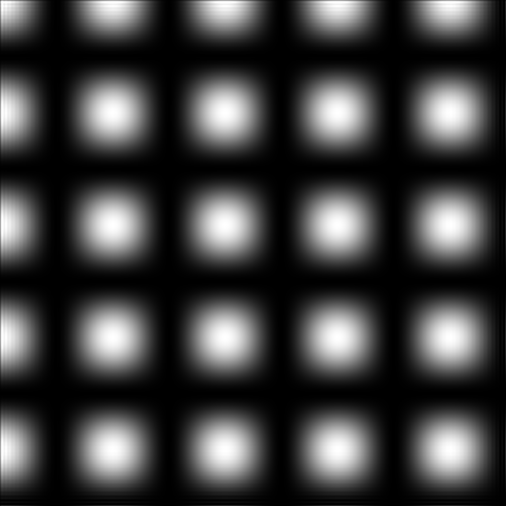
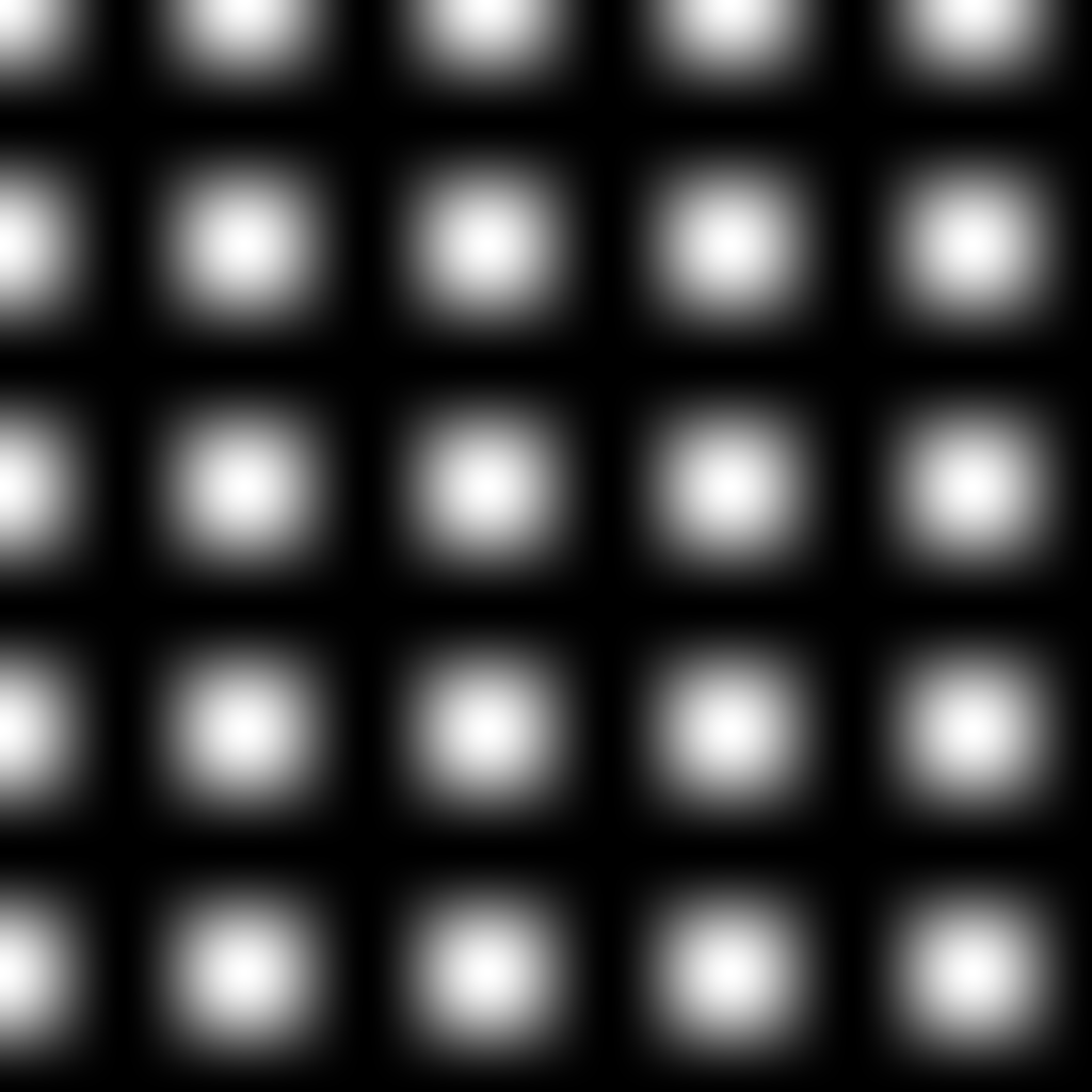
Figure 2: Reconstruction of the function $f_{1}(x,y)=\cos(9x)\cos(9y)$. The second row shows an 8 times zoomed-in version of the upper left corner. Left: original function. Middle: truncated Fourier series with $256^{2}$ Fourier coefficients. Right: GS with DB3 wavelets computed from the same Fourier coefficients.

2.14.1 Fourier samples and wavelet reconstruction

Let

$$\mathrm{T}=\mathrm{S}=\mathrm{L}^{2}(0,1),\qquad\mathrm{S}_{N}=\mathrm{span}\{\psi_{1},\ldots,\psi_{N}\},\quad\mathrm{T}_{M}=\mathrm{span}\{\varphi_{1},\ldots,\varphi_{M}\},$$

where the $\psi_{j}$s are orthonormal complex exponentials spanning $\mathrm{L}^{2}(0,1)$ and the $\varphi_{j}$s are Daubechies wavelets (modified at the boundaries to preserve the vanishing moments) [CDVwavelets]. The advantage of this choice of reconstruction space can be seen by noting that, if $f\in\mathrm{W}^{s}(0,1)$, where $\mathrm{W}^{s}(0,1)$ denotes the usual Sobolev space, then

$$\|f-\mathcal{P}_{\mathrm{T}_{N}}f\|=\mathcal{O}(N^{-s}),\quad N\rightarrow\infty,$$

given that the Daubechies wavelet has sufficiently many vanishing moments. Thus, by using this as the reconstruction space in GS, we are able to obtain a much better approximation to $f$ than the slowly-convergent Fourier series (2.36), provided the stable sampling rate is not too severe. Fortunately, this is not the case:

Theorem 2.27 ([AHPWavelet]).

Let $\mathrm{T}_{M}$ be the reconstruction space consisting of the first $M$ Daubechies wavelet with $q$ vanishing moments on the unit interval and let $\mathrm{S}_{N}$ be the Fourier sampling space as above. Then, for any fixed $\theta\in(1,\infty)$, the stable sampling rate $\Theta(M,\theta)$ is linear in $M$. Furthermore, given any $f\in\mathrm{W}^{s}(0,1)$ with $s\in(0,q)$, the GS approximation $\tilde{f}_{N,M}$ implemented with $N=\Theta(M,\theta)$ samples satisfies

$$\|f-\tilde{f}_{N,M}\|=\mathcal{O}(M^{-s}).$$

This theorem means that GS will have a substantial advantage over classical Fourier series approximations when reconstructing smooth and non-periodic functions. Moreover, recall that the computational complexity of implementing GS in this instance is equivalent to that of the FFT. Hence, one can compute a substantially better approximation to $f$ at little additional expense.

• To illustrate the effectiveness of GS using boundary wavelets, note that by Theorem 2.27 it follows that $\|f-\tilde{f}_{N,M}\|=\mathcal{O}(N^{-s}),$ when $M=\Psi(N,\theta)$ (the stable reconstruction rate) given sufficiently many vanishing moments. This is substantially better than the slow convergence of the truncated Fourier series when the function is non-periodic. To visualize this we have chosen two functions $f_{1}(x,y)=\cos(9x)\cos(9y)$ and $f_{2}(x,y)=xy$. In Figure 2 and Figure 3 we compare the reconstructions via the truncated Fourier series and GS. Note that, as expected from the theory, GS dramatically outperforms the truncated Fourier series given the same samples.

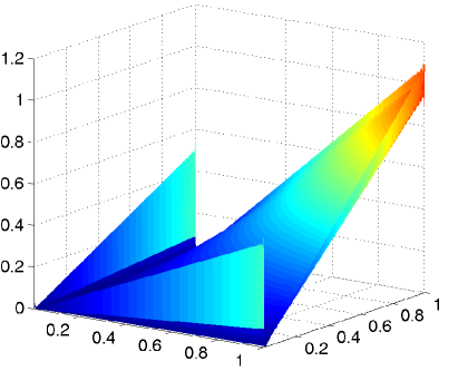
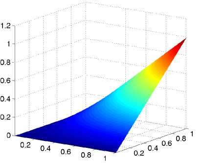
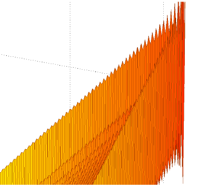
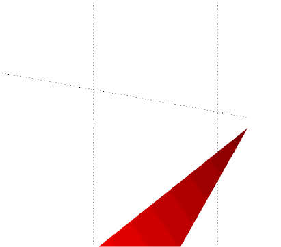
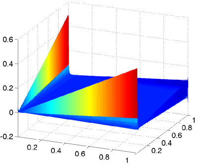
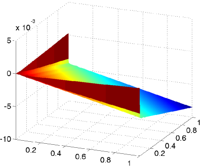
Figure 3: Reconstruction of the function $f_{2}(x,y)=xy$. Upper left: truncated Fourier series with $512^{2}$ Fourier coefficients. Middle left: 8 times zoomed-in version of the upper figure. Lower left: error committed by the truncated Fourier series. Upper right: GS with DB3 wavelets computed from the same $512^{2}$ Fourier coefficients. Middle right: 8 times zoomed-in version of the upper figure. Lower right: error committed by GS.

2.14.2 Fourier samples and polynomial reconstruction

Suppose now we consider the same setup, but we replace the wavelet reconstruction space with the subspace $\mathrm{T}_{M}=\mathrm{span}\{\varphi_{1},\ldots,\varphi_{M}\}$, where $\{\varphi_{j}\}_{j\in\mathbb{N}}$ is the orthonormal basis of Legendre polynomials on $\mathrm{L}^{2}(0,1)$. This space is particularly well suited for smooth and nonperiodic functions. Indeed, suppose that $f$ is analytic in the complex Bernstein ellipse $B(\rho)$ containing $[0,1]$ (here $\rho>1$ is the parameter of the ellipse – see [TrefethenATAP] for details). Then it is well-known that

$$\|f-\mathcal{P}_{\mathrm{T}_{M}}f\|=\mathcal{O}(\rho^{-M}),\quad M\rightarrow\infty.$$

In other words, the expansion of $f$ in orthogonal polynomials converges geometrically fast in $M$. When this space is used in GS, we have the following:

Theorem 2.28 ([BAACHGSCS]).

Let $\mathrm{T}_{M}$ be the reconstruction space consisting of the first $M$ orthonormal Legendre polynomials and let $\mathrm{S}_{N}$ be the Fourier sampling space as above. Then, for any fixed $\theta\in(1,\infty)$, the stable sampling rate $\Theta(M,\theta)$ is quadratic in $M$. In particular, if $f$ is analytic in $B(\rho)$ and the GS approximation $\tilde{f}_{N,M}$ implemented with $N=\Theta(M,\theta)$ samples, then

$$\|f-\tilde{f}_{N,M}\|=\mathcal{O}(\rho^{-M}).$$

• For analytic functions, one may use Legendre polynomials instead of boundary wavelets to improve the reconstruction. From Theorem 2.28 we deduce that for analytic functions we have

  $$\|f-\tilde{f}_{N,M}\|=\mathcal{O}(\rho^{-\sqrt{M}}),$$

  when $M=\Psi(N,\theta)$ (the stable reconstruction rate). As discussed below, this is actually the best possible rate for any recovery algorithm using Fourier data.

  To visualize improvement over the truncated Fourier series, in Figure 4 we display the reconstruction of the function $f(t)=t^{5}e^{-t},$, $t\in[-1,1]$. As is evident, the GS reconstruction with Legendre polynomials is vastly superior to the Fourier series.

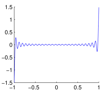
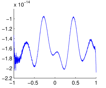
Figure 4: Errors from reconstructions of the function $f(t)=t^{5}e^{-t}$ from $101$ Fourier coefficients. Left: truncated Fourier series. Right: GS.

• Theorem 2.28 states that the GS reconstruction converges root-exponentially fast in the number of samples $N=\mathcal{O}(\sqrt{M})$. Although this is certainly rapid convergence, it is much slower than the convergence rate of the orthogonal projections $\mathcal{P}_{\mathrm{T}_{N}}f$. This is due to the more severe, quadratic scaling of the stable sampling rate.

  Unfortunately, a result proved in [AdcockHansenShadrinStabilityFourier] states that root-exponential convergence is the best possible for any stable method when reconstructing analytic functions from Fourier samples. Moreover, any method with faster convergence must be severely ill-conditioned. Since GS with polynomials attains this stability barrier, it may be considered an optimal method for this problem.

  We note, however, that it is possible to circumvent such a barrier by designing methods which converge only down to a finite, but arbitrarily-small, tolerance. Such methods, although not classically convergent, appear to be most effective in practice for approximating analytic functions. An example of this is the method of Fourier extensions [FEStability], which is based on GS using an oversampled Fourier frame as the reconstruction system.

3 Generalized sampling for inverse and ill-posed problems

Generalized sampling, as introduced in the previous section, reconstructs signals and images from direct measurements, i.e. inner products $\{\langle f,\psi_{j}\rangle\}_{j\in\mathbb{N}}$. In this section address the extension of GS to the case where $f$ is defined additionally through an inverse problem. Note that this was originally presented in [AHHTillposed]. In this section we improve on the results given therein by using the oblique projection analysis developed in the previous section.

To simplify notation, we now drop the $\sim$ symbol from the various reconstructions.

3.1 Introduction

Let $\mathrm{X}$ and $\mathrm{Y}$ be Hilbert spaces and $\mathcal{A}:\mathrm{X}\rightarrow\mathrm{Y}$ a bounded linear operator. We shall suppose that $\mathcal{A}$ is compact, and that it has the singular system $\{\sigma_{k},v_{k},u_{k}\}_{k\in\mathbb{N}}$, where the orthonormal systems $\{v_{k}\}_{k\in\mathbb{N}}$ and $\{u_{k}\}_{k\in\mathbb{N}}$ span the spaces $\mathrm{V}:=N(\mathcal{A})^{\perp}$ and $\mathrm{U}:=N(\mathcal{A}^{*})^{\perp}$ respectively. Here $\mathcal{A}^{*}$ denotes the adjoint of $\mathcal{A}$ and $N(\cdot)$ is the nullity of an operator.

Our aim is to solve the problem

$$\mathcal{A}f=g,\quad f\in\mathrm{X},\ g\in\mathrm{Y},$$ (3.1)

where we are typically faced with noisy data $g^{\delta}=g+z$ with ${\left\|z\right\|}_{\mathrm{Y}}\leq\delta$. In addition, we shall assume that we have frame $\{\psi_{k}\}_{k\in\mathbb{N}}$ for the sampling space $\mathrm{S}:=N(\mathcal{A}^{*})^{\perp}\subseteq\mathrm{Y}$ and a frame $\{\varphi_{k}\}_{k\in\mathbb{N}}$ for the reconstruction space $\mathrm{T}:=N(A)^{\perp}\subseteq\mathrm{X}$. Thus the aim is to reconstruct $f=\sum_{k\in\mathbb{N}}\beta_{k}\varphi_{k}$ in the subspace $\mathrm{T}_{M}=\mathrm{span}\{\varphi_{1},\ldots,\varphi_{M}\}$ (for suitable $M$) from finitely many of the noisy samples

$$S^{*}g^{\delta}=\{\langle g^{\delta},\psi_{k}\rangle\}_{k\in\mathbb{N}}.$$

Recall that $S$ is the synthesis operator for the sampling frame $\{\psi_{k}\}_{k\in\mathbb{N}}$.

Seemingly the most straightforward way in which to do this would be proceed as in standard GS and consider the least-squares data fitting (see (2.35)):

$$\min_{\beta\in P_{M}(\ell^{2}(\mathbb{N}))}\|S^{*}_{R}\mathcal{A}T_{M}\beta-S^{*}_{R}g^{\delta}\|^{2}.$$

Much as in GS (see (2.26)), this would lead to a reconstruction

$$f^{\delta}_{M,R}=T_{M}(T^{*}_{M}\mathcal{A}^{*}S_{R}S^{*}_{R}\mathcal{A}T_{M})^{{\dagger}}T^{*}_{M}\mathcal{A}^{*}S_{R}S^{*}_{R}g^{\delta},$$ (3.2)

where ${\dagger}$ denotes the generalized inverse. However, as already mentioned, the problem can be ill-posed and therefore the generalized inverse in (3.2) need not exist. Hence we are also faced with regularization issues. In what follows, we shall discuss two different regularization treatments of (3.2). Both techniques rely on the singular value decomposition of the operator $\mathcal{A}$. This allows for a splitting into separate sampling and recovery steps. The sampling step in both algorithms is almost the same, whereas the recovery steps are rather different.

In the literature on regularization theory – see, for example [LouisInverse] – there exist similar and successful concepts (e.g. mollifying techniques) but that are primarily designed to obtain approximate/local inversion formulae. It might be rather interesting (but possibly challenging) to discuss these concepts within the framework of sampling theory.

3.2 Regularization by filtering

Let us consider the normal equation $\mathcal{A}^{*}\mathcal{A}f=\mathcal{A}^{*}g$, and let $\mathcal{A}^{{\dagger}}$ denote the generalized inverse of $\mathcal{A}$. If $g\in D(\mathcal{A}^{{\dagger}})$, we can define $f^{{\dagger}}:=\mathcal{A}^{{\dagger}}g$. If $\mathcal{A}$ is injective then it makes sense to define $A^{{\dagger}}:=(\mathcal{A}^{*}\mathcal{A})^{-1}\mathcal{A}^{*}$. Consequently, a stabilized version of $f^{{\dagger}}$ can then be reconstructed as

$$f^{\alpha}:=\mathcal{R}_{\alpha}g,\qquad\mathcal{R}_{\alpha}:=\mathcal{F}_{\alpha}(\mathcal{A}^{*}\mathcal{A})\mathcal{A}^{*}$$ (3.3)

for appropriately chosen filter $\mathcal{F}_{\alpha}$. For an extensive discussion on the choice of $\mathcal{F}_{\alpha}$, see [EnglRegularization, LouisInverse] and references therein. For appropriate $\beta^{\alpha}\in\ell^{2}(\mathbb{N})$ we now have

$$f^{\alpha}=T\beta^{\alpha}=\sum_{k\in\mathbb{N}}\beta^{\alpha}_{k}\varphi_{k}=\mathcal{F}_{\alpha}(\mathcal{A}^{*}\mathcal{A})\mathcal{A}^{*}g=\sum_{k\in\mathbb{N}}\mathcal{F}_{\alpha}(\sigma^{2}_{k})\sigma_{k}\langle g,u_{k}\rangle v_{k}.$$ (3.4)

Let $U$ and $V$ denote the corresponding synthesis operators for the singular system, and denote their adjoints (the analysis operators) by $U^{*}$ and $V^{*}$ respectively. Then

$$(V^{*}f^{\alpha})_{j}=\sum_{k\in\mathbb{N}}\beta^{\alpha}_{k}\langle\varphi_{k},v_{j}\rangle=\sum_{k\in\mathbb{N}}\mathcal{F}_{\alpha}(\sigma^{2}_{k})\sigma_{k}\langle g,u_{k}\rangle\langle v_{k},v_{j}\rangle=\mathcal{F}_{\alpha}(\sigma^{2}_{j})\sigma_{j}\langle g,u_{j}\rangle,$$

and therefore we have

$$V^{*}T\beta^{\alpha}=\Theta_{\alpha}\Sigma\gamma\quad\Longleftrightarrow\quad\Theta^{-1}_{\alpha}V^{*}T\beta^{\alpha}=\Sigma\gamma,$$ (3.5)

where

$$V^{*}T=\left(\begin{array}[]{ccc}\langle\varphi_{1},v_{1}\rangle&\langle\varphi_{2},v_{1}\rangle&\cdots\\ \langle\varphi_{1},v_{2}\rangle&\langle\varphi_{2},v_{2}\rangle&\cdots\\ \vdots&\vdots&\ddots\end{array}\right),\quad\Theta_{\alpha}=\left(\begin{array}[]{ccc}\mathcal{F}_{\alpha}(\sigma^{2}_{1})&0&\cdots\\ 0&\mathcal{F}_{\alpha}(\sigma^{2}_{2})&\cdots\\ \vdots&\vdots&\ddots\end{array}\right),\quad\Sigma=\left(\begin{array}[]{ccc}\sigma_{1}&0&\cdots\\ 0&\sigma_{2}&\cdots\\ \vdots&\vdots&\ddots\end{array}\right).$$

Putting oomputational issues aside for the moment, we note that (3.5) gives a relation for the unknown vector $\beta^{\alpha}$. However, the vector $\gamma=U^{*}g=\{\langle g,u_{j}\rangle\}_{j\in\mathbb{N}}$ is not accessible in practice, and must therefore be related to the known vector of samples $S^{*}g$ of $g$ (or its noisy version $g^{\delta}$). To do this, we observe that

$$\eta=S^{*}g=S^{*}UU^{*}g=S^{*}U\gamma,\quad\mbox{where}\quad S^{*}U=\left(\begin{array}[]{ccc}\langle u_{1},\psi_{1}\rangle&\langle u_{2},\psi_{1}\rangle&\cdots\\ \langle u_{1},\psi_{2}\rangle&\langle u_{2},\psi_{2}\rangle&\cdots\\ \vdots&\vdots&\ddots\end{array}\right).$$

Combining this with (3.5) we now find that $\beta^{\alpha}$ can be obtained as the solution of two infinite-dimensional linear systems of equations:

$$S^{*}U\gamma =S^{*}g,$$ (3.6)

$$\Theta^{-1}_{\alpha}V^{*}T\beta^{\alpha} =\Sigma\gamma.$$ (3.7)

In order to obtain a computable approximation, we need to discretize these equations. For this, we shall use ideas based on GS and uneven sections; specifically, the discussion in §2.10.

3.2.1 Derivation

Suppose first that (3.6) is solved exactly, and we have the samples $U^{*}_{N}g$ at our disposal for some $N\in\mathbb{N}$. Let $M\in\mathbb{N}$ be a second parameter. Then we truncate (3.7) and consider the normal equations:

$$T^{*}_{M}V_{N}\Theta^{-2}_{\alpha,N}V^{*}_{N}T_{M}\beta^{\alpha}_{n,m}=T^{*}_{M}V_{N}\Theta^{-1}_{\alpha,m}\Sigma_{N}U^{*}_{N}g,$$ (3.8)

where $\Theta_{\alpha,N}=P_{N}\Theta_{\alpha}|_{P_{N}(\ell^{2}(\mathbb{N}))}$ and likewise for $\Sigma_{N}$. Assuming $M$ is chosen so that these equations have a unique solution, we then define the reconstruction

$$f^{\alpha}_{N,M}=T_{M}\beta^{\alpha}_{N,M}=\sum^{M}_{j=1}(\beta^{\alpha}_{N,M})_{j}\varphi_{j}.$$ (3.9)

As mentioned, in practice we do not have the samples $U^{*}_{N}g$ at our disposal, hence $f^{\alpha}_{N,M}$ cannot be realized directly. Nevertheless, we can obtain approximations to these values by first solving (3.6). For this, we use a similar approach. Given the noisy samples

$$\eta^{\delta}=S^{*}g^{\delta},$$

we introduce a second parameter $R\in\mathbb{N}$, and define $\gamma^{\delta}_{N,R}\approx U^{*}_{N}g$ as the solution of

$$U^{*}_{N}S_{R}S^{*}_{R}U_{N}\gamma^{\delta}_{N,R}=U^{*}_{N}S_{R}S^{*}_{R}g^{\delta}.$$

If we let

$$g^{\delta}_{N,R}=U_{N}\gamma^{\delta}_{N,R},$$

be the corresponding approximation to $g$, then we can obtain a reconstruction of $f$ that can be realized from the available samples. To do this we set

$$f^{\alpha,\delta}_{N,M,R}=T_{M}\beta^{\alpha,\delta}_{N,M,R},$$

where $\beta^{\alpha,\delta}_{N,M,R}$ is the solution to

$$T^{*}_{M}V_{N}\Theta^{-2}_{\alpha,N}V^{*}_{N}T_{M}\beta^{\alpha,\delta}_{N,M,R}=T^{*}_{M}V_{N}\Theta^{-1}_{\alpha,N}\Sigma_{N}U^{*}_{N}g^{\delta}_{N,R}.$$

3.2.2 Analysis

Our analysis of the regularized reconstruction $f^{\alpha,\delta}_{N,M,R}$ will be based on oblique projections. Let $\mathcal{S}_{R}=S_{R}S^{*}_{R}$ be the partial frame operator for $\{\psi_{j}\}_{j\in\mathbb{N}}$, and define the operator

$$\mathcal{L}^{\alpha}_{N}:\mathrm{X}\rightarrow\mathrm{V}_{N},\qquad\mathcal{L}^{\alpha}_{N}=\sum^{N}_{k=1}\frac{1}{(\mathcal{F}_{\alpha}(\sigma^{2}_{k}))^{2}}\langle\cdot,v_{k}\rangle v_{k}.$$

We also define the subspace angles

$$\theta^{1}_{R,N}=\theta_{\mathrm{U}_{N},\mathcal{S}_{R}(\mathrm{U}_{N})},\qquad\theta^{2,\alpha}_{N,M}=\theta_{\mathrm{T}_{M},\mathcal{L}^{\alpha}_{N}(\mathrm{T}_{M})},$$

as well as

$$\theta^{1}_{\infty,N}=\theta_{\mathrm{U}_{N},\mathcal{S}(\mathrm{U}_{N})},\qquad\theta^{2,\alpha}_{\infty,M}=\theta_{\mathrm{T}_{M},\mathcal{L}^{\alpha}(\mathrm{T}_{M})},$$

where $\mathcal{S}=SS^{*}$ is the infinite frame operator, and

$$\mathcal{L}^{\alpha}=\sum_{k\in\mathbb{N}}\frac{1}{(\mathcal{F}_{\alpha}(\sigma^{2}_{k}))^{2}}\langle\cdot,v_{k}\rangle{v_{k}}.$$

Lemma 3.1.

For fixed $N\in\mathbb{N}$, we have $\theta^{1}_{R,N}\rightarrow\theta^{1}_{\infty,N}$ as $R\rightarrow\infty$. In particular,

$$1\leq\lim_{R\rightarrow\infty}\sec\left(\theta^{1}_{R,N}\right)\leq\sqrt{\frac{c_{2}}{c_{1}}},$$

where $c_{1}$ and $c_{2}$ are the upper and lower frame bounds respectively for the sampling system $\{\psi_{j}\}_{j\in\mathbb{N}}$.

Proof.

This lemma is identical to Lemma 2.20 with $M$ and $N$ replaced by $M$ and $R$ and $\mathrm{T}$ replaced by $\mathrm{U}$. Since $\mathrm{S}=\mathrm{U}$, we have $\cos(\theta_{\mathrm{U}\mathrm{S}})=1$, and the result follows. ∎

Lemma 3.2.

For fixed $M\in\mathbb{N}$, we have $\theta^{2,\alpha}_{N,M}\rightarrow\theta^{2,\alpha}_{\infty,M}$ as $N\rightarrow\infty$. In particular,

$$1\leq\lim_{N\rightarrow\infty}\sec\left(\theta^{2,\alpha}_{N,M}\right)\leq\frac{d_{2}}{d_{1}},$$ (3.10)

where $d_{1}=\inf_{k\in\mathbb{N}}1/\mathcal{F}_{\alpha}(\sigma^{2}_{k})$ and $d_{2}=\sup_{k\in\mathbb{N}}1/\mathcal{F}_{\alpha}(\sigma^{2}_{k})$.

Proof.

Defining the filter $\mathcal{F}_{\alpha}$ as in (3.4), the frame bounds of the frame operator $\mathcal{L}^{\alpha}$ are given by $d_{1}^{2}$, $d_{2}^{2}$ and they are finite and bounded away from zero, i.e. $0<d_{1}^{2}\leq d_{2}^{2}<\infty$. Consequently, we may apply Lemma 2.20 once more to obtain the result. Note that for (3.10) we use the fact that $\mathrm{T}=\mathrm{V}$. ∎

The next lemma relates the reconstructions $f^{\alpha}_{N,M}$ and $f^{\alpha,\delta}_{N,M,R}$ to oblique projections:

Lemma 3.3.

Suppose that $\cos(\theta^{2,\alpha}_{N,M})>0$. Then

$$f^{\alpha}_{N,M}=\mathcal{P}_{\mathrm{T}_{M},(\mathcal{L}^{\alpha}_{N}(\mathrm{T}_{M}))^{\perp}}f^{\alpha},$$

and if $\cos(\theta^{1}_{R,N})>0$, we have

$$f^{\alpha,\delta}_{N,M,R}=\mathcal{P}_{\mathrm{T}_{M},(\mathcal{L}^{\alpha}_{N}(\mathrm{T}_{M}))^{\perp}}\circ\mathcal{R}^{\alpha}\circ\mathcal{P}_{\mathrm{U}_{N},(\mathcal{S}_{R}(\mathrm{U}_{N}))^{\perp}}g^{\delta}.$$

Proof.

The coefficients $\beta^{\alpha}_{N,M}$ of $f^{\alpha}_{N,M}$ are defined by the equations (3.8). Note that $\mathcal{L}^{\alpha}_{N}=V_{N}\Theta^{-2}_{\alpha,N}V^{*}_{N}$. Hence the left-hand side of (3.8) is precisely

$$T^{*}_{M}\mathcal{L}^{\alpha}_{N}f^{\alpha}_{N,M}.$$

For the right-hand side, we first note that

$$\sigma_{k}u_{k}=\frac{1}{\mathcal{F}_{\alpha}(\sigma^{2}_{k})}\mathcal{A}\mathcal{F}_{\alpha}(\mathcal{A}^{*}\mathcal{A})v_{k},$$

and therefore

$$\sigma_{k}\langle g,u_{k}\rangle=\frac{1}{\mathcal{F}_{\alpha}(\sigma^{2}_{k})}\langle\mathcal{F}_{\alpha}(\mathcal{A}^{*}\mathcal{A})\mathcal{A}^{*}g,v_{k}\rangle,$$

which gives

$$\Sigma_{N}U^{*}_{N}g=\Theta^{-1}_{\alpha,N}V^{*}_{N}\mathcal{F}_{\alpha}(\mathcal{A}^{*}\mathcal{A})\mathcal{A}^{*}g=\Theta^{-1}_{\alpha,N}V^{*}_{N}f^{\alpha}.$$

Using this, we find that the right-hand side of (3.8) is precisely

$$T^{*}_{M}V_{N}\Theta^{-1}_{\alpha,N}\Sigma_{N}U^{*}_{N}g=T^{*}_{M}\mathcal{L}^{\alpha}_{N}f^{\alpha}.$$

Hence, using the fact that $\mathcal{L}^{\alpha}_{N}$ is self-adjoint, we find that (3.8) is equivalent to the variational equations

$$\langle f^{\alpha}_{N,M},\mathcal{L}^{\alpha}_{N}\varphi\rangle_{\mathrm{X}}=\langle f^{\alpha},\mathcal{L}^{\alpha}_{N}\varphi\rangle_{\mathrm{X}},\quad\forall\varphi\in\mathrm{T}_{M},\qquad f^{\alpha}_{N,M}\in\mathrm{T}_{N},$$

or equivalently

$$\langle f^{\alpha}_{N,M},\Phi\rangle_{\mathrm{X}}=\langle f^{\alpha},\Phi\rangle_{\mathrm{X}},\quad\forall\Phi\in\mathcal{L}^{\alpha}_{N}(\mathrm{T}_{M}),\qquad f^{\alpha}_{N,M}\in\mathrm{T}_{M},$$

Since $\cos(\theta^{2,\alpha}_{N,M})>0$ these equations have a unique solution whenever $f^{\alpha}\in\mathrm{T}_{0}:=\mathrm{T}_{M}\oplus(\mathcal{L}^{\alpha}_{N}(\mathrm{T}_{M}))^{\perp}$, and it is the oblique projection $\mathcal{P}_{\mathrm{T}_{M},(\mathcal{L}^{\alpha}_{N}(\mathrm{T}_{M}))^{\perp}}f^{\alpha}$ (Lemma 2.13). To obtain the first result, we need only show that $\mathrm{T}_{0}=\mathrm{T}$. For this, we use Lemma 2.12 and note that $\dim(\mathcal{L}^{\alpha}_{N}(\mathrm{T}_{M}))=\dim(\mathrm{T}_{M})$ since $\cos(\theta^{2,\alpha}_{N,M})>0$.

For the second result, let $\beta^{\alpha,\delta}_{N,M,R}$ be the coefficients of $f^{\alpha,\delta}_{N,M,R}$. Arguing as above, we can write

$$\Sigma_{N}U^{*}_{N}g^{\delta}_{N,R}=\Theta^{-1}_{\alpha,N}V^{*}_{N}\mathcal{R}_{\alpha}g^{\delta}_{N,R},$$

and therefore we obtain the following variational form for $f^{\alpha,\delta}_{N,M,R}$:

$$\langle f^{\alpha,\delta}_{N,M,R},\Phi\rangle_{\mathrm{X}}=\langle\mathcal{R}_{\alpha}g^{\delta}_{N,R},\Phi\rangle_{\mathrm{X}},\quad\forall\Phi\in\mathcal{L}^{\alpha}_{N}(\mathrm{T}_{M}),\qquad f^{\alpha,\delta}_{N,M,R}$$

This gives

$$f^{\alpha,\delta}_{N,M,R}=\mathcal{P}_{\mathrm{T}_{M},(\mathcal{L}^{\alpha}_{N}(\mathrm{T}_{M}))^{\perp}}\circ\mathcal{R}_{\alpha}g^{\delta}_{N,R}.$$

To complete the proof, we merely note that $g^{\delta}_{N,R}=\mathcal{P}_{\mathrm{U}_{N},(\mathcal{S}_{R}(\mathrm{U}_{N}))^{\perp}}g^{\delta}$ since $g^{\delta}_{N,R}$ is just the GS reconstruction of $g^{\delta}$ in the subspace $\mathrm{U}_{N}$ from the samples $S^{*}_{R}g^{\delta}$. ∎

We are now in a position to state and prove the main results for this approximation:

Theorem 3.4.

Suppose that $\cos(\theta^{2,\alpha}_{N,M})>0$. Then $f^{\alpha}_{N,M}$ exists uniquely and satisfies the sharp bounds

$$\|f^{\alpha}_{N,M}\|_{\mathrm{X}}\leq\sec\left(\theta^{2,\alpha}_{N,M}\right)\|f^{\alpha}\|_{\mathrm{X}},$$

and

$$\|f^{\alpha}-f^{\alpha}_{N,M}\|_{\mathrm{X}}\leq\sec\left(\theta^{2,\alpha}_{N,M}\right)\|f^{\alpha}-\mathcal{P}_{\mathrm{T}_{M}}f^{\alpha}\|_{\mathrm{X}}.$$

Furthermore, we have

$$\|f^{{\dagger}}-f^{\alpha}_{N,M}\|_{\mathrm{X}}\leq\left(1+2\sec\left(\theta^{2,\alpha}_{N,M}\right)\right)\|f^{{\dagger}}-f^{\alpha}\|_{\mathrm{X}}+\sec\left(\theta^{2,\alpha}_{N,M}\right)\|f^{{\dagger}}-\mathcal{P}_{\mathrm{T}_{M}}f^{{\dagger}}\|_{\mathrm{X}}.$$

Proof.

The first and second estimates follow from Corollary 2.11 with $\mathrm{U}=\mathrm{T}_{M}$ and $\mathrm{V}=\mathcal{L}_{N}^{\alpha}(\mathrm{T}_{M})^{\perp}$. The third estimate can be easily achieved as follows. We have

$$\|f^{{\dagger}}-f^{\alpha}_{N,M}\|_{\mathrm{X}} \leq\|f^{{\dagger}}-f^{\alpha}\|_{\mathrm{X}}+\|f^{\alpha}-f^{\alpha}_{N,M}\|_{\mathrm{X}}$$

$$=\|f^{{\dagger}}-f^{\alpha}\|_{\mathrm{X}}+\sec\left(\theta^{2,\alpha}_{N,M}\right)\|f^{\alpha}-\mathcal{P}_{\mathrm{T}_{M}}f^{\alpha}\|_{\mathrm{X}}$$

$$\leq\|f^{{\dagger}}-f^{\alpha}\|_{\mathrm{X}}+\sec\left(\theta^{2,\alpha}_{N,M}\right)\left(\|(I-\mathcal{P}_{\mathrm{T}_{M}})(f^{{\dagger}}-f^{\alpha})\|_{\mathrm{X}}+\|(I-\mathcal{P}_{\mathrm{T}_{M}})f^{{\dagger}}\|_{\mathrm{X}}\right)$$

$$=\left(1+2\sec\left(\theta^{2,\alpha}_{N,M}\right)\right)\|f^{{\dagger}}-f^{\alpha}\|_{\mathrm{X}}+\sec\left(\theta^{2,\alpha}_{N,M}\right)\|f^{{\dagger}}-\mathcal{P}_{\mathrm{T}_{M}}f^{{\dagger}}\|_{\mathrm{X}}.$$

as required. ∎

Theorem 3.5.

Suppose that $\cos(\theta^{1}_{R,N})>0$ and $\cos(\theta^{2,\alpha}_{N,M})>0$. Then

$$\|f^{{\dagger}}-f^{\alpha,\delta}_{N,M,R}\|_{\mathrm{X}}\leq\|f^{{\dagger}}-f^{\alpha}_{N,M}\|_{\mathrm{X}}+C^{\alpha}_{N,M,R}\left(\|f-\mathcal{P}_{\mathrm{V}_{N}}f\|_{\mathrm{X}}+\delta\right),$$

where

$$C^{\alpha}_{N,M,R}\leq\sec\left(\theta^{2,\alpha}_{N,M}\right)\sec\left(\theta^{1}_{R,N}\right)\sigma_{N+1}\max_{k=1,\ldots,N}\left\{\mathcal{F}_{\alpha}(\sigma^{2}_{k})\sigma_{k}\right\}.$$

Proof.

By the triangle inequality, we have

$$\|f^{{\dagger}}-f^{\alpha,\delta}_{N,M,R}\|_{\mathrm{X}}\leq\|f^{{\dagger}}-f^{\alpha}_{N,M}\|_{\mathrm{X}}+\|f^{\alpha}_{N,M}-f^{\alpha,\delta}_{N,M,R}\|_{\mathrm{X}}.$$ (3.11)

It suffices to consider the second term. By Lemma 3.3, we have

$$f^{\alpha,\delta}_{N,M,R} =\mathcal{P}_{\mathrm{T}_{M},(\mathcal{L}^{\alpha}_{N}(\mathrm{T}_{M}))^{\perp}}\circ\mathcal{R}_{\alpha}\circ\mathcal{P}_{\mathrm{U}_{N},(\mathcal{S}_{R}(\mathrm{U}_{N}))^{\perp}}g^{\delta}$$

$$=f^{\alpha}_{N,M}+\mathcal{P}_{\mathrm{T}_{M},(\mathcal{L}^{\alpha}_{N}(\mathrm{T}_{M}))^{\perp}}\left(\mathcal{R}_{\alpha}\circ\mathcal{P}_{\mathrm{U}_{N},(\mathcal{S}_{R}(\mathrm{U}_{N}))^{\perp}}g^{\delta}-f^{\alpha}\right)$$

$$=f^{\alpha}_{N,M}+\mathcal{P}_{\mathrm{T}_{M},(\mathcal{L}^{\alpha}_{N}(\mathrm{T}_{M}))^{\perp}}\circ\mathcal{R}_{\alpha}\left(\mathcal{P}_{\mathrm{U}_{N},(\mathcal{S}_{R}(\mathrm{U}_{N}))^{\perp}}g^{\delta}-g\right)$$

$$=f^{\alpha}_{N,M}+\mathcal{P}_{\mathrm{T}_{M},(\mathcal{L}^{\alpha}_{N}(\mathrm{T}_{M}))^{\perp}}\circ\mathcal{P}_{\mathrm{V}_{N}}\circ\mathcal{R}_{\alpha}\left(\mathcal{P}_{\mathrm{U}_{N},(\mathcal{S}_{R}(\mathrm{U}_{N}))^{\perp}}g^{\delta}-g\right).$$

Thus, an application of Theorem 2.10 gives

$$\|f^{\alpha}_{N,M}-f^{\alpha,\delta}_{N,M,R}\|_{\mathrm{X}} \leq\sec\left(\theta^{2,\alpha}_{N,M}\right)\left\|\mathcal{P}_{\mathrm{V}_{N}}\circ\mathcal{R}_{\alpha}\left(\mathcal{P}_{\mathrm{U}_{N},(\mathcal{S}_{R}(\mathrm{U}_{N}))^{\perp}}g^{\delta}-g\right)\right\|_{\mathrm{X}}$$

$$\leq\sec\left(\theta^{2,\alpha}_{N,M}\right)\|\mathcal{P}_{\mathrm{V}_{N}}\circ\mathcal{R}_{\alpha}\|_{\mathrm{Y}\rightarrow\mathrm{X}}\|\mathcal{P}_{\mathrm{U}_{N},(\mathcal{S}_{R}(\mathrm{U}_{N}))^{\perp}}g^{\delta}-g\|_{\mathrm{Y}}.$$ (3.12)

Consider the final term of this expression. We have

$$\|\mathcal{P}_{\mathrm{U}_{N},(\mathcal{S}_{R}(\mathrm{U}_{N}))^{\perp}}g^{\delta}-g\|_{\mathrm{Y}} \leq\|g-\mathcal{P}_{\mathrm{U}_{N},(\mathcal{S}_{R}(\mathrm{U}_{N}))^{\perp}}g\|_{\mathrm{Y}}+\|\mathcal{P}_{\mathrm{U}_{N},(\mathcal{S}_{R}(\mathrm{U}_{N}))^{\perp}}(g-g^{\delta})\|_{\mathrm{Y}}$$

$$\leq\sec\left(\theta^{1}_{R,N}\right)\left(\|g-\mathcal{P}_{\mathrm{U}_{N}}g\|_{\mathrm{Y}}+\|g-g^{\delta}\|_{\mathrm{Y}}\right).$$

Substituting this into (3.12) and recalling that $g^{\delta}=g+z$ with $\|z\|_{\mathrm{Y}}\leq\delta$ gives

$$\|f^{\alpha}_{N,M}-f^{\alpha,\delta}_{N,M,R}\|_{\mathrm{X}}\leq\sec\left(\theta^{2,\alpha}_{N,M}\right)\sec\left(\theta^{1}_{R,N}\right)\|\mathcal{P}_{\mathrm{V}_{N}}\circ\mathcal{R}_{\alpha}\|_{\mathrm{Y}\rightarrow\mathrm{X}}\left(\|g-\mathcal{P}_{\mathrm{U}_{N}}g\|_{\mathrm{Y}}+\delta\right).$$ (3.13)

To complete the proof, we make the following two claims. First,

$$\|\mathcal{P}_{\mathrm{V}_{N}}\circ\mathcal{R}_{\alpha}\|_{\mathrm{Y}\rightarrow\mathrm{X}}\leq\max_{k=1,\ldots,N}\left\{\mathcal{F}_{\alpha}(\sigma^{2}_{k})\sigma_{k}\right\},$$ (3.14)

and second,

$$\|g-\mathcal{P}_{\mathrm{U}_{N}}g\|_{\mathrm{Y}}\leq\sigma_{N+1}\|f-\mathcal{P}_{\mathrm{V}_{N}}f\|_{\mathrm{X}}.$$ (3.15)

For (3.14), let $h\in\mathrm{U}$ be arbitrary and write $h=U\beta$ for some $\beta\in l^{2}(\mathbb{N})$ with ${\left\|\beta\right\|}=\|h\|_{\mathrm{Y}}$. Then

$$\mathcal{P}_{\mathrm{V}_{N}}\circ\mathcal{R}_{\alpha}h=\sum^{N}_{k=1}\mathcal{F}_{\alpha}(\sigma^{2}_{k})\sigma_{k}\beta_{k}v_{k},$$

and therefore

$$\|\mathcal{P}_{\mathrm{V}_{N}}\circ\mathcal{R}_{\alpha}h\|_{\mathrm{X}}\leq\max_{k=1,\ldots,N}\left\{\mathcal{F}_{\alpha}(\sigma^{2}_{k})\sigma_{k}\right\}\|h\|_{\mathrm{Y}},$$

which gives (3.14). Now consider (3.15). Since $g=\mathcal{A}f$, we have $\langle g,u_{k}\rangle=\sigma_{k}\langle f,v_{k}\rangle$, and therefore

$$\|g-\mathcal{P}_{\mathrm{U}_{N}}g\|^{2}_{\mathrm{Y}}=\sum_{k>N}|\langle g,u_{k}\rangle|^{2}=\sum_{k>N}\sigma^{2}_{k}|\langle f,v_{k}\rangle|^{2}\leq\sigma^{2}_{N+1}\|f-\mathcal{P}_{\mathrm{V}_{N}}f\|^{2}_{\mathrm{X}},$$

as required. Combining (3.13)–(3.15) gives the result. ∎

Note that, much as with standard GS, the various subspaces angles in the error bounds can be controlled by appropriately varying $N$, $M$ and $R$. This is a consequence of Lemmas 3.1 and 3.2.

3.3 Regularization by uneven sections

The approach in the previous section was essentially based on the normal equation $\mathcal{A}^{*}\mathcal{A}f=\mathcal{A}^{*}g$. As an alternative, we now propose an approach based on directly utilizing the singular value decomposition of $\mathcal{A}$. Since $\mathcal{A}=U\Sigma V^{*}$, we may write

$$\eta=S^{*}g=S^{*}U\Sigma V^{*}T\beta=S^{*}U\gamma,$$

where $f=T\beta$ as in the previous section. As in the previous approach, we may reformulate this as the two linear equations

$$S^{*}U\gamma=S^{*}g$$ (3.16)

$$V^{*}T\beta=\Sigma^{-1}\gamma.$$ (3.17)

We now proceed in a similar manner by discretizing both these equations. Using (3.16), we construct the following approximation to $g$:

$$g^{\delta}_{N,R}=U_{N}(U^{*}_{N}S_{R}S^{*}_{R}U_{N})^{-1}U^{*}_{N}S_{R}S^{*}_{R}g^{\delta},$$

and using (3.17) we construct an approximation to $f$:

$$f_{N,M}=T_{M}(T^{*}_{M}V_{N}V^{*}_{N}T_{M})^{{\dagger}}T^{*}_{M}V_{N}\Sigma^{-1}_{N}U^{*}_{N}g.$$

Much as before, $f_{N,M}$ cannot be realized from the available sampling data, and therefore we combine these two approximations to give the final approximation

$$f^{\delta}_{N,M,R}=T_{M}(T^{*}_{M}V_{N}V^{*}_{N}T_{M})^{{\dagger}}T^{*}_{M}V_{N}\Sigma^{-1}_{N}U^{*}_{N}g^{\delta}_{N,R}.$$

3.3.1 Analysis

We proceed in a similar manner to that of the previous approach. Let $\theta^{1}_{R,N}$ be as in the previous section, and define the new subspace angles

$$\theta^{2}_{N,M}=\theta_{\mathrm{T}_{M},\mathcal{P}_{\mathrm{V}_{N}}(\mathrm{T}_{M})}.$$

Much as before, this angle can be controlled by varying $N$ and $M$ appropriately:

Lemma 3.6.

For fixed $M\in\mathbb{N}$, we have $\theta^{2}_{N,M}\rightarrow 1$ as $N\rightarrow\infty$.

We now require the following lemma:

Lemma 3.7.

Suppose that $\cos(\theta^{2}_{N,M})>0$. Then

$$f_{N,M}=\mathcal{P}_{\mathrm{T}_{M},(\mathcal{P}_{\mathrm{V}_{N}}(\mathrm{T}_{M}))^{\perp}}f,$$

and if additionally $\cos(\theta^{1}_{R,N})>0$, then we have

$$f^{\delta}_{N,M,R}=\mathcal{P}_{\mathrm{T}_{M},(\mathcal{P}_{\mathrm{V}_{N}}(\mathrm{T}_{M}))^{\perp}}\circ(\mathcal{A}^{*}\mathcal{A})^{{\dagger}}\mathcal{A}^{*}\circ\mathcal{P}_{\mathrm{U}_{N},(\mathcal{S}_{R}(\mathrm{U}_{N}))^{\perp}}g^{\delta}.$$

Proof.

Note first that the coefficients $\beta_{N,M}$ and $\beta_{N,M,R}$ of $f_{N,M}$ and $f_{N,M,R}$ respectively satisfy

$$T^{*}_{M}V_{N}V^{*}_{N}T_{M}\beta_{N,M}=T^{*}_{M}V_{N}\Sigma^{-1}_{N}U^{*}_{N}g,$$ (3.18)

and

$$T^{*}_{M}V_{N}V^{*}_{N}T_{M}\beta_{N,M,R}=T^{*}_{M}V_{N}\Sigma^{-1}_{N}U^{*}_{N}g^{\delta}_{N,R}.$$ (3.19)

Moreover, we have

$$T^{*}_{M}V_{N}V^{*}_{N}=T^{*}_{M}\mathcal{P}_{\mathrm{V}_{N}},$$ (3.20)

and, since $u_{k}=\sigma_{k}\mathcal{A}(\mathcal{A}^{*}\mathcal{A})^{{\dagger}}v_{k}$,

$$V_{N}\Sigma^{-1}_{N}U^{*}_{N}h=V_{N}V^{*}_{N}(\mathcal{A}^{*}\mathcal{A})^{{\dagger}}\mathcal{A}^{*}h=\mathcal{P}_{\mathrm{V}_{N}}(\mathcal{A}^{*}\mathcal{A})^{{\dagger}}\mathcal{A}^{*}h,\quad h\in\mathrm{U}.$$ (3.21)

In particular,

$$V_{N}\Sigma^{-1}_{N}U^{*}_{N}g=\mathcal{P}_{\mathrm{V}_{N}}f.$$ (3.22)

Substituting (3.20) and (3.22) into (3.18), we deduce that (3.18) is equivalent to the variational problem

$$\langle f_{N,M},\mathcal{P}_{\mathrm{V}_{N}}\varphi\rangle_{\mathrm{X}}=\langle f,\mathcal{P}_{\mathrm{V}_{N}}\varphi\rangle_{\mathrm{X}},\quad\forall\varphi\in\mathrm{T}_{M}.$$

Thus $f_{N,M}=\mathcal{P}_{\mathrm{T}_{M},\mathcal{P}_{\mathrm{V}_{N}}(\mathrm{T}_{M})}f$ by Lemma 2.13 and the fact that $\cos(\theta^{2}_{n,m})>0$. Now consider $f^{\delta}_{N,M,R}$. Substituting (3.20) and (3.21) with $h=g_{N,R}$ into (3.19), we immediately deduce that

$$f^{\delta}_{N,M,R}=\mathcal{P}_{\mathrm{T}_{M},(\mathcal{P}_{\mathrm{V}_{N}}(\mathrm{T}_{M}))^{\perp}}\circ(\mathcal{A}^{*}\mathcal{A})^{{\dagger}}\mathcal{A}^{*}g^{\delta}_{N,R},$$

and the result now follows from the fact that $g^{\delta}_{N,R}=\mathcal{P}_{\mathrm{U}_{N},(\mathcal{S}_{R}(\mathrm{U}_{N}))^{\perp}}g^{\delta}$. ∎

We are now able to provide the main result:

Theorem 3.8.

Suppose that $\cos(\theta^{1}_{R,N})>0$ and $\cos(\theta^{2}_{N,M})>0$. Then

$$\|f^{\dagger}-f^{\delta}_{N,M,R}\|_{\mathrm{X}} \leq (1+2\sec(\theta^{2}_{N,M}))\|f^{\dagger}-f\|_{\mathrm{X}}+\sec(\theta^{2}_{N,M})\|f^{\dagger}-\mathcal{P}_{\mathrm{T}_{M}}f^{\dagger}\|_{\mathrm{X}}$$

$$\quad\quad+\sec\left(\theta^{2}_{N,M}\right)\sec\left(\theta^{1}_{R,N}\right)\left(\|f-\mathcal{P}_{\mathrm{V}_{N}}f\|_{\mathrm{X}}+\frac{\delta}{\sigma_{N}}\right).$$

Proof.

We have

$$\|f^{\dagger}-f^{\delta}_{N,M,R}\|_{\mathrm{X}}\leq\|f^{\dagger}-f\|_{\mathrm{X}}+\|f-f_{N,M}\|_{\mathrm{X}}+\|f_{N,M}-f^{\delta}_{N,M,R}\|_{\mathrm{X}}.$$

By the previous lemma, the second term yields

$$\|f-f_{N,M}\|_{\mathrm{X}} \leq \sec(\theta^{2}_{N,M})\|f-\mathcal{P}_{\mathrm{T}_{M}}f\|_{\mathrm{X}}$$

$$\leq \sec(\theta^{2}_{N,M})(2\|f^{\dagger}-f\|_{\mathrm{X}}+\|f^{\dagger}-\mathcal{P}_{\mathrm{T}_{M}}f^{\dagger}\|_{\mathrm{X}}).$$

So we now consider the third term. We have

$$\|f_{N,M}-f^{\delta}_{N,M,R}\|_{\mathrm{X}} =\|\mathcal{P}_{\mathrm{T}_{M},(\mathcal{P}_{\mathrm{V}_{N}}(\mathrm{T}_{M}))^{\perp}}\left(f-(\mathcal{A}^{*}\mathcal{A})^{{\dagger}}\mathcal{A}^{*}\circ\mathcal{P}_{\mathrm{U}_{N},(\mathcal{S}_{r}(\mathrm{U}_{N}))^{\perp}}\circ g^{\delta}\right)\|_{\mathrm{X}}$$

$$=\|\mathcal{P}_{\mathrm{T}_{M},(\mathcal{P}_{\mathrm{V}_{N}}(\mathrm{T}_{M}))^{\perp}}\mathcal{P}_{\mathrm{V}_{N}}\left(f-(\mathcal{A}^{*}\mathcal{A})^{{\dagger}}\mathcal{A}^{*}\circ\mathcal{P}_{\mathrm{U}_{N},(\mathcal{S}_{r}(\mathrm{U}_{N}))^{\perp}}\circ g^{\delta}\right)\|_{\mathrm{X}}$$

$$\leq\sec\left(\theta^{2}_{N,M}\right)\|\mathcal{P}_{\mathrm{V}_{N}}(\mathcal{A}^{*}\mathcal{A})^{{\dagger}}\mathcal{A}^{*}\|_{\mathrm{Y}\rightarrow\mathrm{X}}\|g-\mathcal{P}_{\mathrm{U}_{N},(\mathcal{S}_{R}(\mathrm{U}_{N}))^{\perp}}g^{\delta}\|_{\mathrm{Y}}$$

$$\leq\sec\left(\theta^{2}_{N,M}\right)\|\mathcal{P}_{\mathrm{V}_{N}}(\mathcal{A}^{*}\mathcal{A})^{{\dagger}}\mathcal{A}^{*}\|_{\mathrm{Y}\rightarrow\mathrm{X}}\sec\left(\theta^{2}_{N,R}\right)\left(\|g-\mathcal{P}_{\mathrm{U}_{N}}g\|_{\mathrm{Y}}+\delta\right).$$ (3.23)

Let $h\in\mathrm{U}$. Then

$$\|\mathcal{P}_{\mathrm{V}_{N}}(\mathcal{A}^{*}\mathcal{A})^{{\dagger}}\mathcal{A}^{*}h\|^{2}_{\mathrm{X}}=\sum^{N}_{k=1}|\langle(\mathcal{A}^{*}\mathcal{A})^{{\dagger}}\mathcal{A}^{*}h,v_{k}\rangle_{\mathrm{X}}|^{2}=\sum^{N}_{k=1}\frac{1}{\sigma^{2}_{k}}|\langle h,u_{k}\rangle_{\mathrm{Y}}|^{2}\leq\frac{1}{\sigma^{2}_{N}}\|h\|^{2}_{\mathrm{Y}}.$$

Hence $\|\mathcal{P}_{\mathrm{V}_{N}}(\mathcal{A}^{*}\mathcal{A})^{{\dagger}}\mathcal{A}^{*}\|_{\mathrm{Y}\rightarrow\mathrm{X}}\leq 1/\sigma_{N}$. Combining this with (3.23) and (3.15) and the fact that $\sigma_{N+1}\leq\sigma_{N}$ now gives the result. ∎

3.4 Numerical Examples

In this section we test the frameworks proposed in the previous subsections. First, we discuss a one-dimensional example for which we analyze the suggested regularized and non-regularized reconstruction methods. Thereafter, we consider a two-dimensional experiment. The goal is to verify that we can achieve, even in the presence of noise, a reasonable reconstruction by the proposed sampling-recovery technique.

• In order illustrate the proposed sampling theorems (Theorem 3.5 and 3.8), we consider the linear operator $\mathcal{A}:\mathrm{L}^{2}([0,1])\rightarrow\mathrm{L}^{2}([0,1])$ defined by

  $$g(t)=\mathcal{A}f(t)=\int_{0}^{t}f(s)\,ds\ ,$$

  with singular system $\{\sigma_{k},v_{k},u_{k}\}$ given by

  $$\sigma_{k}=\frac{1}{(k+1/2)\pi}~{},\hskip 15.0ptv_{k}=\sqrt{2}\cos(k+1/2)\pi t~{},\hskip 15.0ptu_{k}=\sqrt{2}\sin(k+1/2)\pi t\ .$$

  Note that $\{v_{k}\}_{k\in\mathbb{N}}$ and $\{u_{k}\}_{k\in\mathbb{N}}$ form orthonormal systems for $\mathrm{L}^{2}([0,1])$. To keep technicalities at a reasonable level, we choose the Fourier basis as both the recovery system $\{\varphi_{k}\}_{k\in\mathbb{Z}}$ and sampling system $\{\psi_{k}\}_{k\in\mathbb{Z}}$, i.e.

  $$\varphi_{k}(t)=e^{2\pi ikt}~{}~{}~{}~{}~{}~{}\text{and}~{}~{}~{}~{}~{}~{}\psi_{k}(t)=e^{2\pi ikt}\ .$$

  Let the signal $f$ to be reconstructed be defined by $f(t)=\cos 2\pi t$. Consequently, $f$ can be expanded as follows,

  $$f(t)=T\beta=\sum_{k\in\mathbb{Z}}\beta_{k}e^{2\pi ikt}=\frac{1}{2}e^{2\pi i(-1)t}+\frac{1}{2}e^{2\pi i(+1)t}~{},$$

  and in particular, $\beta_{-1}=1/2$, $\beta_{1}=1/2$, and $\beta_{k}=0$ for $k\in\mathbb{Z}\setminus\{-1,+1\}$. Moreover, the data $g$ are given through $g(t)=\mathcal{A}f(t)=1/(2\pi)\sin 2\pi t$. In this particular example we also have explicit expression for all further required quantities,

  $$\gamma = U^{*}g=\{\gamma_{l}\}_{l\in\mathbb{N}}=\left\{\frac{4\sqrt{2}\cos(l\pi)}{\pi^{2}(4l^{2}+4l-15)}\right\}_{l\in\mathbb{N}}$$

  $$\eta = S^{*}g=\{\eta_{k}\}_{k\in\mathbb{Z}}~{}\text{with}~{}\eta_{-1}=\frac{-i}{4\pi}~{},~{}\eta_{+1}=\frac{i}{4\pi}~{}\text{and}~{}\eta_{k}=0,~{}k\not=\pm 1$$

  $$V^{*}T = \left(\frac{\sqrt{2}((l\pi+\pi/2)\cos(l\pi)-2\pi ik)}{(2\pi ik)^{2}+(l\pi+\pi/2)^{2}}\right)_{l\in\mathbb{N},k\in\mathbb{Z}}$$

  $$S^{*}U = \left(\frac{(-1)^{l+1}\sqrt{2}((l\pi+\pi/2)\cos(l\pi)+2\pi ik)}{(2\pi ik)^{2}+(l\pi+\pi/2)^{2}}\right)_{k\in\mathbb{Z},l\in\mathbb{N}}~{}.$$

  The approximations to $f$ from the $R$ samples $S^{*}_{R}g^{\delta}$ are now given by by

  $$f^{\alpha,\delta}_{N,M,R} = \mathcal{P}_{\mathrm{T}_{M},(\mathcal{L}^{\alpha}_{N}(\mathrm{T}_{M}))^{\perp}}\circ\mathcal{R}^{\alpha}\circ\mathcal{P}_{\mathrm{U}_{N},(\mathcal{S}_{R}(\mathrm{U}_{N}))^{\perp}}g^{\delta}~{}~{}~{}\text{and}$$

  $$f^{\delta}_{N,M,R} = \mathcal{P}_{\mathrm{T}_{M},(\mathcal{P}_{\mathrm{V}_{N}}(\mathrm{T}_{M}))^{\perp}}\circ(\mathcal{A}^{*}\mathcal{A})^{{\dagger}}\mathcal{A}^{*}\circ\mathcal{P}_{\mathrm{U}_{N},(\mathcal{S}_{R}(\mathrm{U}_{N}))^{\perp}}g^{\delta}~{}.$$

  For the first approximation we shall consider filtering by Tikhonov regularization, i.e. the entries in $\Theta_{\alpha,N}$ are given by $\mathcal{F}_{\alpha}(\sigma_{k}^{2})=1/(\alpha+\sigma_{k}^{2})$.

  We discuss now several different recovery scenarios. In the first case we choose a fixed (and reasonable) setting for $N$, $M$ and $R$ and vary the noise level $\delta$. We then compare the recovery quality of $f^{\alpha,\delta}_{N,M,R}$ and $f^{\delta}_{N,M,R}$ while experimentally tuning the regularization parameter $\alpha$ towards optimal recovery. This experiment shall show that for a fixed number of data samples and coefficients in the series expansion of the solution an optimal choice of regularization parameter induces a substantially improved recovery.

  In the second case we fix the number $M$ of coefficients in series expansion of the solution and try to find for different noise levels $\delta$ reasonable integers $N$ and $R$ to derive $f^{\delta}_{N,M,R}$. For the same numbers $M$ and $R$ we then experimentally determine an optimal $\alpha$ to compute $f^{\alpha,\delta}_{N,M,R}$. This experiment shall show that a reasonable choice of $N$ and $R$ may feasibly stabilize the recovery and providing approximations that cannot be significantly improved by a fine tuning of $\alpha$.

  First case: vary $z=g-g^{\delta}$ such the relative error $\varepsilon_{rel}=100\cdot\|z\|/\|g\|$ is 0%, 5% and 10% and let $M=20$, $N=30$ and $R=40$. The numerical results are illustrated in the following table and visualized in Figures 5,6, and 7.
  

  $\varepsilon_{rel}$, $\delta$	$\|f-f^{\delta}_{20,30,40}\|$	$\|f-f^{0,\delta}_{20,30,40}\|$	$\|f-f^{\alpha_{opt},\delta}_{20,30,40}\|$	$\alpha_{opt}$	Fig.
  0%, 0	0.6262	0.4995	0.0071	0.00017	5
  5%, 0.0056	1.1738	0.9728	0.1536	0.00037	6
  10%, 0.0113	1.7593	1.5268	0.2265	0.00061	7

  

  

  

  

  

  

  

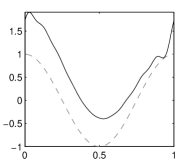
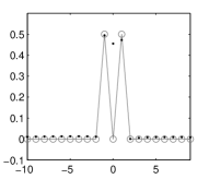
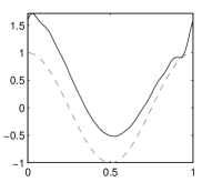
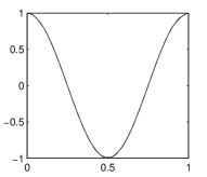
  Figure 5: Recovery results for $\varepsilon_{rel}$ = 0%. Top (from left to right): $\eta^{\delta}=S^{*}_{R}(g+z)$ ($\cdot$) and $S^{*}_{R}U_{N}\gamma$ ($\circ$), $\beta^{\delta}_{20,30,40}$ ($\cdot$) and $\beta$ ($\circ$), $f^{\delta}_{20,30,40}=T_{n}\beta^{\delta}_{20,30,40}$ (–) and $f$ (- -). Bottom (from left to right): $\beta^{0,\delta}_{20,30,40}$ ($\cdot$) and $\beta$ ($\circ$), $f^{0,\delta}_{20,30,40}=T_{M}\beta^{0,\delta}_{20,30,40}$ (–) and $f$ (- -), $\beta^{\alpha_{opt},\delta}_{20,30,40}$ ($\cdot$) and $\beta$ ($\circ$), $f^{\alpha_{opt},\delta}_{20,30,40}=T_{M}\beta^{\alpha_{opt},\delta}_{20,30,40}$ (–) and $f$ (- -).

  

  

  

  

  

  

  

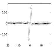
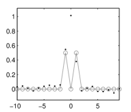
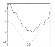
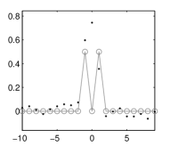
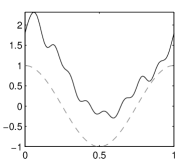
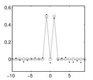
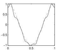
  Figure 6: Recovery results for $\varepsilon_{rel}$ = 5%. Top (from left to right): $\eta^{\delta}=S^{*}_{r}(g+z)$ ($\cdot$) and $S^{*}_{R}U_{N}\gamma$ ($\circ$), $\beta^{\delta}_{20,30,40}$ ($\cdot$) and $\beta$ ($\circ$), $f^{\delta}_{20,30,40}=T_{M}\beta^{\delta}_{20,30,40}$ (–) and $f$ (- -). Bottom (from left to right): $\beta^{0,\delta}_{20,30,40}$ ($\cdot$) and $\beta$ ($\circ$), $f^{0,\delta}_{20,30,40}=T_{M}\beta^{0,\delta}_{20,30,40}$ (–) and $f$ (- -), $\beta^{\alpha_{opt},\delta}_{20,30,40}$ ($\cdot$) and $\beta$ ($\circ$), $f^{\alpha_{opt},\delta}_{20,30,40}=T_{M}\beta^{\alpha_{opt},\delta}_{20,30,40}$ (–) and $f$ (- -).

  

  

  

  

  

  

  

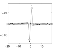
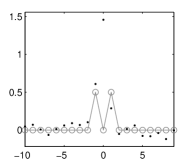
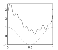
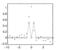
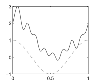
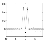
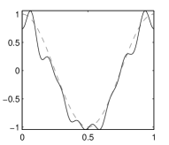
  Figure 7: Recovery results for $\varepsilon_{rel}$ = 10%. Top (from left to right): $\eta^{\delta}=S^{*}_{R}(g+z)$ ($\cdot$) and $S^{*}_{R}U_{N}\gamma$ ($\circ$), $\beta^{\delta}_{20,30,40}$ ($\cdot$) and $\beta$ ($\circ$), $f^{\delta}_{20,30,40}=T_{M}\beta^{\delta}_{20,30,40}$ (–) and $f$ (- -). Bottom (from left to right): $\beta^{0,\delta}_{20,30,40}$ ($\cdot$) and $\beta$ ($\circ$), $f^{0,\delta}_{20,30,40}=T_{M}\beta^{0,\delta}_{20,30,40}$ (–) and $f$ (- -), $\beta^{\alpha_{opt},\delta}_{20,30,40}$ ($\cdot$) and $\beta$ ($\circ$), $f^{\alpha_{opt},\delta}_{20,30,40}=T_{M}\beta^{\alpha_{opt},\delta}_{20,30,40}$ (–) and $f$ (- -).

  Second case: we first fix $M=10$ and ask then, for different relative errors $\varepsilon_{rel}\in\{0\%,5\%,10\%\}$, for an adequate choice (numerically determined) of $N$ and $R$ in order to derive an optimal approximation $f^{\delta}_{N,M,R}$. Then, we try by fine tuning $\alpha$ to obtain with $f^{\alpha,\delta}_{N,M,R}$ a comparable or possibly better approximation. The results are documented in the following table. The illustrations of this experiment are given in Figure 8 (the illustrations for $\varepsilon_{rel}=0\%$ are not provided since there is no visual difference).

  $\varepsilon_{rel}$, $\delta$	$N$	$R$	$\|f-f^{\delta}_{N,10,R}\|$	$\|f-f^{0,\delta}_{N,10,R}\|$	$\|f-f^{\alpha_{opt},\delta}_{N,10,R}\|$	$\alpha_{opt}$	Fig.
  0%, 0.0	10	1000	0.002114839173	0.002114839160	0.000112	0.0000035	-
  5%, 0.0042	40	100	0.0303	0.0433	0.0371	0.000025	8
  10%, 0.0075	40	80	0.1044	0.2990	0.2732	0.0001	8

  

  

  

  

  

  

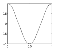
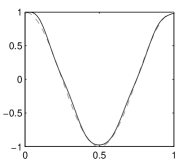
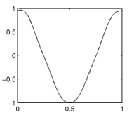
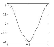
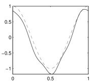
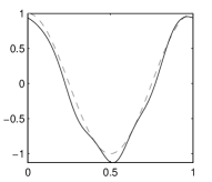
  Figure 8: Experimental results for $\varepsilon_{rel}=5\%$: $f^{\delta}_{10,40,100}$ (t.l.), $f^{0,\delta}_{10,40,100}$ (t.m.), $f^{0.000025,\delta}_{10,40,100}$ (t.r.), and for $\varepsilon_{rel}=10\%$: $f^{\delta}_{10,40,100}$ (b.l.), $f^{0,\delta}_{10,40,100}$ (b.m.), $f^{0.0001,\delta}_{10,40,100}$ (b.r.). In all subfigures the dashed line (- -) represents the true solution $f$.

• In the second example we discuss the Radon transform

  $$Rf(\tau,\omega)=\int_{-\sqrt{1-\tau^{2}}}^{+\sqrt{1-\tau^{2}}}f(\tau\omega+t\omega^{\perp})dt~{}~{},$$ (3.24)

  where we assume in this example that ${\rm supp}(f)\subset D=\{x\in\mathbb{R}^{2}:~{}\|x\|\leq 1\}$, and $\omega\in S^{1}$, $\tau\in[-1,1]$, see [LouisInverse]. The map $R$ is linear and continuous (with norm $\sqrt{4\pi}$) between $\mathrm{L}^{2}(D)$ and $\mathrm{L}^{2}([-1,1]\times[0,2\pi],g^{-1})$, with weight function $g(\tau)=\sqrt{1-\tau^{2}}$. As a map between these spaces, the Radon transform has the following singular system (for details see again [LouisInverse]),

  $$\{(v_{ml},u_{ml},\sigma_{ml}):~{}m\geq 0,l\in\mathbb{Z}:|l|\leq m,m+l~{}{\rm even}~{}\}~{}~{},$$

  $$v_{m,l}(x) = \left\{\begin{array}[]{ll}\sqrt{\frac{m+1}{\pi}}\|x\|^{|l|}P^{(0,|l|)}_{(m-|l|)/2}(2\|x\|^{2}-1)Y_{l}(x/\|x\|)&\|x\|\leq 1\\ 0&\|x\|>1\end{array}\right.$$

  $$u_{m,l}(\tau,\omega) = \left\{\begin{array}[]{ll}\frac{1}{\pi}g(\tau)U_{m}(\tau)Y_{l}(\omega)&|\tau|\leq 1\\ 0&|\tau|>1\end{array}\right.$$

  $$\sigma_{m,l} = 2\sqrt{\frac{\pi}{m+1}}$$

  where

  $$P^{(\alpha,\beta)}_{n}(x)=\frac{\Gamma(\alpha+n+1)}{n!\Gamma(\alpha+\beta+n+1)}\sum_{m=0}^{n}\left(\begin{array}[]{c}n\\ m\end{array}\right)\frac{\Gamma(\alpha+\beta+n+m+1)}{\Gamma(\alpha+m+1)}\left(\frac{x-1}{2}\right)^{m}~{}~{},$$

  $$U_{m}(\tau)=\frac{\sin((m+1)\arccos(\tau))}{\sin(\arccos(\tau))}~{}.$$

  Hence, for each $f\in\mathrm{L}^{2}(D)$, we have $Rf=\sum_{m,l}=\sigma_{ml}\langle f,v_{ml}\rangle_{\mathrm{L}^{2}(D)}u_{ml}$. We choose as recovery system for $\mathrm{L}^{2}(D)=\mathrm{L}^{2}(rdrd\theta,[0,1]\times[0,2\pi])$ the separable Haar basis on $[0,1]\times[0,2\pi]$,

  $$\varphi_{\lambda}(r,\theta)=\psi^{\rm Haar}_{\lambda_{1}}(r)\psi^{\rm Haar}_{\lambda_{2}}(\theta)~{},~{}\lambda_{i}=(q_{i},j,k_{i})~{}~{},~{}$$

  where $q_{i}$ prescribes the species of the wavelet ($q_{i}=0$ - generator, $q_{i}=1$ - corresponding wavelets, $i=1,2$), $j\in\mathbb{Z}$ the scales, and $(k_{1},k_{2})\in I$ the translations. Then, we obtain

  $$\langle f,v_{ml}\rangle_{\mathrm{L}^{2}(D)} = \int_{D}f(x)v_{ml}(x)dx=\int_{0}^{2\pi}\int_{0}^{1}f(r\cos\theta,r\sin\theta)\bar{v}_{ml}(r\cos\theta,r\sin\theta)rdrd\theta$$

  $$= \int_{0}^{2\pi}\int_{0}^{1}f(r\cos\theta,r\sin\theta)\sqrt{\frac{m+1}{\pi}}r^{|l|}P^{(0,|l|)}_{(m-|l|)/2}(2r^{2}-1)e^{-il\theta}rdrd\theta$$

  $$= \sum_{\lambda}\beta_{\lambda}\int_{0}^{2\pi}\psi_{\lambda_{2}}(\theta)e^{-il\theta}d\theta\sqrt{\frac{m+1}{\pi}}\int_{0}^{1}\psi_{\lambda_{1}}(r)r^{|l|+1}P^{(0,|l|)}_{(m-|l|)/2}(2r^{2}-1)dr$$

  $$= \sum_{\lambda}\beta_{\lambda}(V^{*}T)_{\lambda,ml}~{}.$$

  As sampling system, we choose an orthonormal Fourier-Mellin-type basis, $\{\psi_{n,k}\}_{(n,k)\in\mathbb{N}\times\mathbb{Z}}$, to span $\mathrm{L}^{2}([-1,1]\times[0,2\pi],g^{-1})$, which we define by

  $$\psi_{n,k}(\tau,\theta)=\frac{1}{4}\sqrt{\frac{\tau+1}{\alpha_{n}\pi}}Q_{n}((\tau+1)/2)e^{i\theta k}g^{1/2}(\tau)~{}~{},$$ (3.27)

  where

  $$\alpha_{n}=\frac{1}{2(n+1)}~{},~{}~{}Q_{n}(\tau)=\sum_{p=0}^{n}\alpha_{n,p}\tau^{p}~{},~{}~{}\alpha_{n,p}=(-1)^{n+1}\frac{(n+p+1)!}{(n-p)!p!(p+1)!}~{}~{}.$$

  Therefore,

  $$(S^{*}U)_{nk,ml}=\delta_{lk}\,\cdot\,\frac{1}{2}\int_{-1}^{1}U_{m}(\tau)\sqrt{\frac{\tau+1}{\alpha_{n}\pi}}Q_{n}((\tau+1)/2)g^{1/2}(\tau)d\tau~{}.$$

  The phantom function $f$ to be recovered is now simulated on $D$ by placing $N$ ellipses,

  $$E^{k}=\left\{x\in\mathbb{R}^{2}:\left\|\left(\begin{array}[]{cc}a^{k}&0\\ 0&b^{k}\end{array}\right)\left(\begin{array}[]{cc}\cos\nu^{k}&\sin\nu^{k}\\ -\sin\nu^{k}&\cos\nu^{k}\end{array}\right)\left(x-x^{k}\right)\right\|\leq r^{k}\right\}~{},~{}~{}~{}~{}k=1,\ldots,N~{}~{},$$

  through,

  $$f^{0}(x)=0~{},~{}~{}~{}f^{n+1}(x)=f^{n}(x)\,\chi_{D\setminus E^{n+1}}(x)+\xi^{n+1}\,\chi_{E^{n+1}}(x)~{},~{}~{}~{}n=0,\ldots,N-1~{}{\rm and}~{}~{}f(x):=f^{N}(x)~{}.$$

  The $k$-th ellipse is specified by a set of parameters $\Pi^{k}=(x^{k},r^{k},\nu^{k},a^{k},b^{k},\xi^{k})$, where $x_{k}$ determines the localization, $r^{k}$ the radius, $\nu^{k}$ the orientation, $a^{k},b^{k}$ the semi-axes, and $\xi^{k}$ the plateau height.

  In our particular example we selected three ellipses,

  $$E^{1} : \Pi^{1}=\left(0.5,0.0,0.3,-\pi/12,1,0.5,2\right)$$

  $$E^{2} : \Pi^{2}=\left(-0.5,0.0,0.3,\pi/12,1,0.5,2\right)$$

  $$E^{3} : \Pi^{3}=\left(0,-0.4,0.3,\pi/2,2,0.6,3\right)~{},$$

  resulting in a phantom function $f(x)=f^{3}(x)$ which visualized in figure 9. The resolutions (which can be made as fine as desired) to represent $f$ (on a cartesian and/or polar grid) as well as $Rf$ are restricted in our computational experiments to equispaced grids of size $256\times 256$ and $512\times 512$. This is of course not fine enough when significantly increasing the number of recovery, singular and sampling functions. In particular, the singular and sampling functions contain oscillatory components that indeed require a much finer resolution. But as we focus here on exemplarily documenting the applicability of the proposed approach, we restrict ourselves to problem dimensions that cause no extra sophistication when dealing with very large systems.

  

  

  

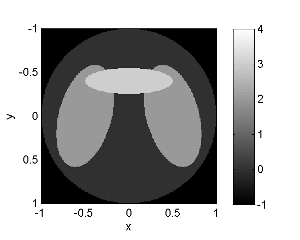
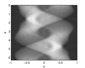
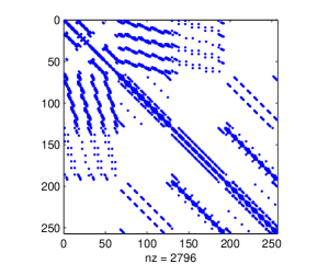
  Figure 9: Left: phantom function $f$ on $D$, middle: Radon transform $Rf$ for $m\leq 30$ (resulting in $496$ singular functions), right: matrix $T^{*}_{256}V_{496}\Theta^{-2}_{\alpha,496}W_{256}V^{*}_{496}T_{256}$, where for the wavelet system the scale is limited to $2\leq j\leq 3$ (resulting in 256 basis functions).

  The approximation to $f$ is now obtained through

  $$f^{\alpha,\delta}_{N,M,R}=\mathcal{P}_{\mathrm{T}_{M},(\mathcal{L}^{\alpha}_{N}(\mathrm{T}_{M}))^{\perp}}\circ\mathcal{R}^{\alpha}\circ\mathcal{P}_{\mathrm{U}_{N},(\mathcal{S}_{R}(\mathrm{U}_{N}))^{\perp}}g^{\delta}~{}.$$

  We have derived $f^{\alpha,\delta}_{N,M,R}$ within the following scenarios, for visual inspection see figure 10,

  	$MR$	$N$		$E(f,f^{\alpha,\delta}_{N,M,R})$, rel.
  	(wavelet functions)	(singular functions)	(sampling functions)	recovery error
  scenario 1	1024 ($2\leq j\leq 4$)	1326	1681	22.03 %
  scenario 2	4096 ($2\leq j\leq 5$)	4186	4225	15.62 %
  scenario 3	16384 ($2\leq j\leq 6$)	16471	16641	11.40 %

  

  

  

  

  

  

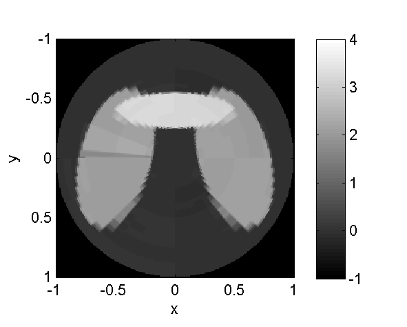
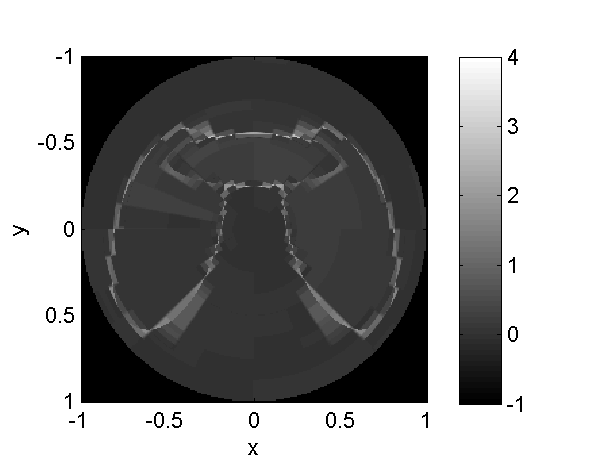
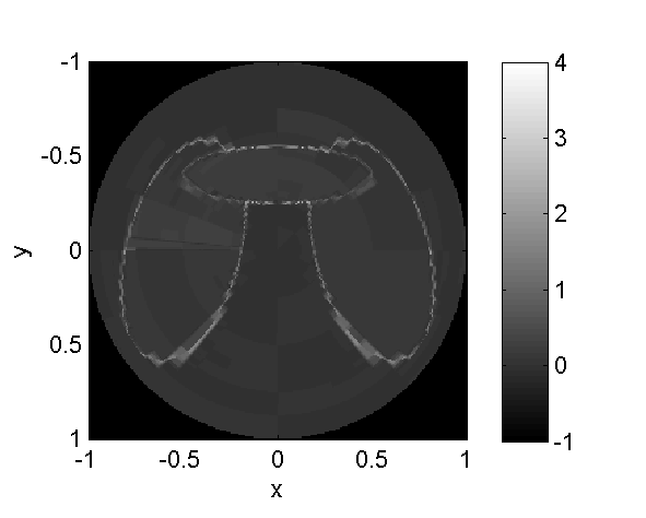
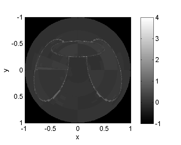
  Figure 10: Top row (from left to right): recoveries of $f$ by $f^{\alpha,\delta}_{1024,1326,1681}$ (scenario 1), $f^{\alpha,\delta}_{4096,4186,4225}$ (scenario 2), $f^{\alpha,\delta}_{16384,16471,16641}$ (scenario 3), where the relative error is $\varepsilon_{rel}=5\%$ and the corresponding Tikhonov stabilization is fine tuned by $\alpha=0.00001$. Bottom row (from left to right): modulus of difference between $f$ and $f^{\alpha,\delta}_{1024,1326,1681}$, $f^{\alpha,\delta}_{4096,4186,4225}$, and $f^{\alpha,\delta}_{16384,16471,16641}$.

  In our particular example the relative data error is $\varepsilon_{rel}=5\%$ and the corresponding Tikhonov stabilization is fine tuned by $\alpha=0.00001$. The relative recovery error is defined in this experiment by

  $$E(f,f^{\alpha,\delta}_{N,M,R})=\frac{\|f-f^{\alpha,\delta}_{N,M,R}\|_{\mathrm{L}^{2}(D)}}{\|f\|_{\mathrm{L}^{2}(D)}}~{}.$$

4 Compressed sensing over the continuum

In §2 and §3 we addressed reconstruction problems where an unknown signal was measured according to a frame or basis and its coefficients were sought in another frame or basis. A key facet of this was that, despite the infinite-dimensionality of the signal (i.e. it lies in a separable Hilbert space), we have access to only finitely-many measurements. As the main theorems illustrate, by appropriately varying the relevant parameters according to the stable sampling rate, we obtain stable, and in some sense, optimal reconstructions.

Thus far, we have not assumed any particular structure for on the unknown signal. The aim of this final section is to do precisely this. We shall show that when the signal $f$ possesses a sparsity-type structure, it is possible to obtain vastly improved reconstructions than with standard GS using the same total number of measurements. The key to this will be an extension of compressed sensing (CS) principles to the continuum (i.e. infinite-dimensional) setting.

4.1 Compressed sensing

Let us first briefly review standard CS theory [candesCSMag, donohoCS, EldarKutyniokCSBook, FoucartRauhutCSbook]. A typical CS setup, and one which is most relevant for our purposes, is as follows. Let $\{\psi_{j}\}^{N}_{j=1}$ and $\{\varphi_{j}\}^{N}_{j=1}$ be two orthonormal bases of $\mathbb{C}^{N}$, the sampling and sparsity bases respectively, and write

$$A=\left(u_{ij}\right)^{N}_{i,j=1}\in\mathbb{C}^{N\times N},\qquad u_{ij}=\langle\varphi_{j},\psi_{i}\rangle.$$

Note that the matrix $A$, the change-of-basis matrix, is an isometry of $\mathbb{C}^{N}$. Let $f\in\mathbb{C}^{N}$ be an unknown signal, and suppose that

$$f=\sum^{N}_{j=1}\beta_{j}\varphi_{j},$$

for coefficients $\beta=(\beta_{1},\ldots,\beta_{N})^{\top}$. Then we have the linear relation

$$A\beta=\hat{f},$$ (4.1)

where $\hat{f}=(\hat{f}_{1},\ldots,\hat{f}_{N})^{\top}$ and

$$\hat{f}_{j}=\langle f,\psi_{j}\rangle,\quad j=1,\ldots,N,$$ (4.2)

are the samples of $f$. Here $\langle\cdot,\cdot\rangle$ denotes the usual inner product on $\mathbb{C}^{N}$.

Whilst one could solve the linear system (4.1) to find $\beta$, the goal of CS is to recover $f$ using only $m\ll N$ of the measurements (4.2). To do this, CS relies on three key principles:

• Sparsity,

• Incoherence,

• Uniform random subsampling.

Let us now introduce these concepts:

Definition 4.1 (Sparsity).

A signal $f\in\mathbb{C}^{N}$ is said to be $s$-sparse in the orthonormal basis $\{\varphi_{j}\}^{N}_{j=1}$ if at most $s$ of its coefficients in this basis are nonzero. In other words, $f=\sum^{N}_{j=1}\beta_{j}\varphi_{j}$, and the vector $\beta\in\mathbb{C}^{N}$ satisfies $|\mathrm{supp}(x)|\leq s$, where

$$\mathrm{supp}(\beta):=\{j:\beta_{j}\neq 0\}.$$

Definition 4.2 (Incoherence).

Let $A=(a_{ij})^{N}_{i,j=1}\in\mathbb{C}^{N\times N}$ be an isometry. The coherence of $A$ is

$$\mu(A)=\max_{i,j=1,\ldots,N}|a_{ij}|^{2}\in[N^{-1},1].$$ (4.3)

We say that $A$ is incoherent if $\mu(A)$ is small, and perfectly incoherent if $\mu(A)=N^{-1}$.

Suppose a signal $f$ is sparse in a basis $\{\varphi_{j}\}^{N}_{j=1}$. CS theory states that $f$ can be recovered exactly (with probability at least $1-\epsilon$) from $m$ measurements subsampled uniformly at random subsampled, i.e. from the collection

$$\{\hat{f}_{j}:j\in\Omega\},$$

where $\Omega\subseteq\{1,\ldots,N\}$, $|\Omega|=m$ is chosen uniformly at random, provided $m$ satisfies

$$m\gtrsim\mu(A)\cdot N\cdot s\cdot\left(1+\log(\epsilon^{-1})\right)\cdot\log N,$$ (4.4)

(see [Candes_Plan] and [BAACHGSCS]). Moreover, reconstruction of $f$ can be achieved by practical numerical algorithms. For example, one may solve the convex optimization problem

$$\min_{\eta\in\mathbb{C}^{N}}\|\eta\|_{l^{1}}\ \mbox{subject to $P_{\Omega}A\eta=P_{\Omega}\hat{f}$},$$ (4.5)

where $P_{\Omega}\in\mathbb{C}^{N\times N}$ is the diagonal projection matrix with $j^{\mathrm{th}}$ entry $1$ if $j\in\Omega$ and zero otherwise. Critically, if sampling and sparsity systems are sufficiently incoherent, in particular, if $\mu(A)=\mathcal{O}\left(N^{-1}\right)$, then we find from (4.4) that $m$ need only be proportional to the sparsity $s$ times by a logarithmic factor in $N$. In situations where $s\ll N$, which is often the case in practice, this translates into a substantial saving in the number of required measurements over the linear approach based on (4.1). Note that the scaling $\mu(A)=\mathcal{O}\left(N^{-1}\right)$ is achieved if, for example, $A$ is the DFT matrix.

It goes without saying that these fundamental results were groundbreaking when they were introduced, and have generated a new field of sparse approximation with CS at its core. However, there are some drawbacks. Notably, the standard theory of CS is finite dimensional: it concerns the recovery of sparse vectors in vector spaces. On the other hand, a large class of inverse problems are based on an infinite-dimensional framework. As we have discussed, important examples occur in applications such as medical imaging, due primarily to the physics behind the measurement systems used in X-ray tomography and Magnetic Resonance Imaging (MRI), as well as radar, sonar and microscopy.

Putting sparsity aside for the moment, let us note a key difference between the finite- and infinite-dimensional cases. In finite dimensions there is an invertible linear system (4.1) which allows $f$ to be recovered exactly from its full set of measurements. However, in infinite dimensions, where the set of measurements is countably infinite, there is no such way to recover $f$ exactly. Thus, before sparsity can be even considered, one must first address the question of how to recover $f$ from a finite subset of its measurements. Fortunately, the work in §2 and §3 has shown precisely how to address this problem: namely, by using generalized sampling. The developments we make in this section are directly based on this: namely, they show how to extend GS to exploit subsampling, thus culminating in a framework for infinite-dimensional CS.

Perhaps surprisingly, when making this generalization of CS to the infinite-dimensional setting, the three principles of the finite-dimensional case – namely, sparsity, incoherence and uniform random subsampling – must be dispensed with and replaced by new principles. In particular, we shall explain why neither sparsity nor incoherence are witnessed for analog problems, and consequently why an alternate sampling strategy is required. In order to develop the new theory, we therefore replace these principles with three new concepts:

• Asymptotic sparsity,

• Asymptotic incoherence,

• Multilevel random subsampling.

The remainder of this section is devoted to developing these principles and the new theory based on them. Specifically, in §4.3–4.5 we introduce these concepts and explain their relevance to practical problems. Next, in §4.7 we introduce the new theory based on these principles. Finally, in §4.8–4.10 we discuss three important consequences of these new concepts. These consequences, summarized in Figure 11, are at odds with the conceived wisdom stemming from finite-dimensional CS.

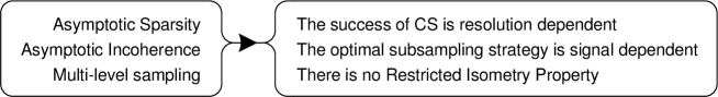
Figure 11: Consequences of the new principles.

4.2 Discrete models and crimes

Before doing this, let us first illustrate why it is important to adopt an infinite-dimensional model. In short, the reason for this is the following. The standard discrete models used in CS, which are based on the discrete Fourier and discrete wavelet transforms, result in mathematical crimes (the inverse and wavelet crimes respectively), and this leads to substandard reconstructions when applied to real data, or, perhaps more perniciously, artificially good reconstructions with inappropriately simulated data. Fortunately the infinite-dimensional CS framework we develop later allows one to avoid both these crimes, and thereby obtain better reconstructions. Moreover, even in situations where such crimes may be tolerated (e.g. problems with low SNR), we shall see that in order to properly understand the behaviour of the resulting algorithms one must also use the infinite-dimensional framework (see §4.6).

We now discuss the two aforementioned crimes.

4.2.1 The inverse crime

The inverse crime [hansen_discrete_2010, Kaipio, Mller, GLPU] in the setting of Fourier sampling stems from two numerical discretizations. The first is when one assumes a pixel model for the unknown signal $f$, i.e.

$$f=\sum^{N}_{j=1}\tilde{\beta}_{j}\varphi_{j},\quad N\in\mathbb{N},$$ (4.6)

where the $\varphi_{j}$s are step functions. The second (and most serious part of the crime) comes from substituting (4.6) into (1.1) and then replacing the integral by a Riemann sum. This results in the discretization of (1.1):

$$y=U_{\mathrm{df}}\tilde{\beta},\qquad\tilde{\beta}=(\tilde{\beta}_{1},\ldots,\tilde{\beta}_{N})^{\top},$$

where $U_{\mathrm{df}}\in\mathbb{C}^{N\times N}$ denotes the discrete Fourier transform. Note that the crime here stems from the fact that the vector $y$ has nothing to do with the actual samples of $f$ arising from its continuous Fourier transform. Indeed, the vector $y$ is a rather poor approximation to the vector of point samples of $\mathcal{F}f$ [GLPU].

4.2.2 The wavelet crime

The so-called wavelet crime [StrangNguyen] is the following phenomenon. Given a function $f\in L^{2}(\mathbb{R})$, a scaling function $\varphi$ and a mother wavelet $\psi$, we are interested in obtaining the the wavelet coefficients of $f$ via the discrete wavelet transform. However, instead of assuming that $f=\sum_{j=-\infty}^{\infty}\beta_{j}\varphi(\cdot-j)$ and computing the wavelet coefficients from the exact values $\{\beta_{j}\}$ via the discrete wavelet transform, one simply replaces the $\beta_{j}$s by pointwise samples of $f$. As Strang and Nguyen put it: “Is this legal? No, it is a wavelet crime.” [StrangNguyen, p. 232]. As we will see in the examples below, the use of the wavelet crime in CS may cause artefacts and unnecessarily slow convergence.

4.2.3 The inverse and wavelet crimes in finite-dimensional compressed sensing

In problems where one encounters samples of the Fourier transform of a signal $f$, it is typical to assume that $f$ is sparse in a wavelet basis. To fit this into the usual finite-dimensional CS framework, it is standard to discretize according to the discrete Fourier and wavelet transforms, and solve

$$\min_{\eta\in\mathbb{C}^{2N}}\|\eta\|_{l^{1}}\ \mbox{subject to}\ \ P_{\Omega}U_{\mathrm{df}}V^{-1}_{\mathrm{dw}}\eta=P_{\Omega}\hat{f},$$ (4.7)

or some variant thereof in the case of data corrupted by noise. Here, critically, $\hat{f}$ is the vector of the first $2N$ continuous Fourier samples of the function $f$.

Since $f$ is sparse in a wavelet basis, the hope is that (4.7) recovers the coefficients of $f$ exactly. However, the use of the discrete wavelet and Fourier transforms introduces two crimes into the reconstruction (4.7). As we now explain, this has a catastrophic effect on (4.7) and means that sparse signals $f$ cannot in fact be recovered exactly by (4.7). See Example 4.2.5 for a numerical illustration of this phenomenon.

To explain why this occurs, let us first consider the matrix $U^{-1}_{\mathrm{df}}$. This matrix maps the vector of Fourier coefficients $\hat{f}$ of a function $f$ to a vector consisting of pointwise values on an equispaced $2N$-grid of points in $[0,1]$. However, this mapping commits an error: for an arbitrary function $f$, the result is only an approximation to the grid values of $f$. The question is, how large is this error, and how does it affect (4.7) and its solutions? To understand this, let $x\in\mathbb{C}^{2N}$ be the vector defined by

$$U_{\mathrm{df}}x=\hat{f}.$$

It is simple to see that $x$ consists precisely of the values of the function

$$f_{N}(t)=\epsilon\sum^{N}_{j=-N+1}\mathcal{F}f(j\epsilon)\mathrm{e}^{2\pi\mathrm{i}\epsilon jt},\quad\epsilon=1/2,$$ (4.8)

on the equispaced $2N$-grid. Since this function is nothing more than the truncated Fourier series of $f$, one deduces that the approximation resulting from modelling the continuous Fourier transform with $U_{\mathrm{df}}$ is equivalent to replacing a function $f$ by its partial Fourier series $f_{N}$.

Let us now consider the discrete wavelet transform $x_{0}\in\mathbb{C}^{2N}$ of $x$:

$$x_{0}=V_{\mathrm{dw}}x.$$

The right-hand side of the equality constraint in (4.7) now reads

$$P_{\Omega}U_{\mathrm{df}}V^{-1}_{\mathrm{dw}}x_{0}.$$

Thus, for the method (4.7) to be successful, i.e. to recover sparse vectors of wavelet coefficients, we require $x_{0}=V_{\mathrm{dw}}x$ to be a sparse vector. Unfortunately this can never happen. Sparsity of $x_{0}$ is equivalent to stipulating that the partial Fourier series $f_{N}$ be sparse in a wavelet basis. However, whilst $f$ was assumed to be sparse in a wavelet basis, the function $f_{N}$ consists of smooth complex exponentials. Hence it cannot have a sparse representation in a wavelet basis.

4.2.4 Infinite-dimensional compressed sensing

The approach (4.7) is loosely based on the principle of discretizing first and then applying finite-dimensional tools, and its failures described above can be accredited to the poor discretizations of the discrete Fourier and wavelet transforms. As an alternative, we now introduce the infinite-dimensional CS approach to avoid these issues. This is loosely based on the principle of first formulating the reconstruction problem in infinite dimensions, and then discretizing in a careful manner.

Suppose that $\{\varphi_{j}\}_{j\in\mathbb{N}}$ is the given orthonormal sparsity system (e.g. a wavelet basis), and let $\{\psi_{j}\}_{j\in\mathbb{N}}$ be an orthonormal sampling basis (e.g. the Fourier bais). If

$$f=\sum_{j\in\mathbb{N}}\beta_{j}\varphi_{j},$$

then, as described in §2, the unknown vector of coefficients $\beta=\{\beta_{j}\}_{j\in\mathbb{N}}$ is the solution of

$$A\beta=\hat{f},$$

where

$$A=\left(\begin{array}[]{ccc}\left<\varphi_{1},\psi_{1}\right>&\left<\varphi_{2},\psi_{1}\right>&\cdots\\ \left<\varphi_{1},\psi_{2}\right>&\left<\varphi_{2},\psi_{2}\right>&\cdots\\ \vdots&\vdots&\ddots\end{array}\right),$$

and $\hat{f}=\{\hat{f}_{j}\}_{j\in\mathbb{N}}$ is the infinite vector of samples of $f$. Let $\Omega\subseteq\mathbb{N}$ be a set of indices of size $|\Omega|=m\in\mathbb{N}$ and suppose that we have access to the samples $\{\hat{f}_{j}:j\in\Omega\}.$ The goal is to recover the vector $\beta$ from these samples. To do so, we we first formulate the infinite-dimensional optimization problem

$$\inf_{\eta\in\ell^{1}(\mathbb{N})}\|\eta\|_{\ell^{1}}\ \mbox{subject to}\ \ P_{\Omega}A\eta=P_{\Omega}\hat{f}.$$ (4.9)

Note that no crimes have been committing in formulating (4.9), and we shall see below that if $f$ is $s$-sparse then, under appropriate conditions on $\Omega$ (e.g. it is chosen randomly according to an appropriate distribution), $f$ can be recovered exactly from (4.9). Unfortunately, besides some special circumstances, we cannot solve (4.9) numerically. Thus having formulated the problem in infinite dimensions, we now discretize. For this, we follow the same ideas that lead to GS. We introduce an additional parameter $K\in\mathbb{N}$ and consider the finite-dimensional optimization problem

$$\min_{\eta\in P_{K}(\ell^{2}(\mathbb{N}))}\|\eta\|_{l^{1}}\ \mbox{subject to}\ \ P_{\Omega}AP_{K}\eta=P_{\Omega}\hat{f}.$$ (4.10)

We refer to this as infinite-dimensional CS. Much as with GS, the parameter $K$ must be sufficiently large so as to ensure a good reconstruction. To see this, we note the following [BAACHGSCS, Prop. 7.4]:

Proposition 4.3.

Let $A\in\mathcal{B}(\ell^{2}(\mathbb{N}))$, $\beta\in\ell^{1}(\mathbb{N})$ and $P_{\Omega}\in\mathcal{B}(\ell^{2}(\mathbb{N}))$ be a finite-rank projection. Then, for all sufficiently large $K\in\mathbb{N}$, there exists an $\xi_{K}$ satisfying

$$\|\xi_{K}\|_{\ell^{1}}=\inf_{\eta\in\ell^{1}(\mathbb{N})}\left\{\|\eta\|_{\ell^{1}}:P_{\Omega}AP_{K}\eta=P_{\Omega}A\beta\right\}.$$

Moreover, for each $\epsilon>0$ there is a $K_{0}\in\mathbb{N}$ such that, whenever $K\geq K_{0}$, we have $\|\xi_{K}-\tilde{\xi}_{K}\|_{\ell^{1}}<\epsilon$, where $\tilde{\xi}_{K}$ satisfies

$$\|\tilde{\xi}_{K}\|_{\ell^{1}}=\inf_{\eta\in\ell^{1}(\mathbb{N})}\left\{\|\eta\|_{\ell^{1}}:P_{\Omega}A\eta=P_{\Omega}A\beta\right\}.$$ (4.11)

In particular, if there is a unique minimizer $\xi$ of (4.11) then $\xi_{K}\rightarrow\xi$ in the $\ell^{1}$-norm.

This proposition means that computed solutions of (4.10) approximate those of (4.9) for large $K$. Thus, for the purposes of analysis, we may consider (4.9), whereas (4.10) is used in computations.

Before presenting an example of (4.10), we now briefly remark on one particular difference between (4.10) and finite-dimensional approach (4.7). First, let us denote the bandwidth of the sampling set $\Omega$ by $M\in\mathbb{N}$, i.e. $M$ is the smallest number for which $\Omega\subseteq\{1,\ldots,M\}$. Then the matrix in (4.10) is a subsampled version of the uneven section

$$P_{M}UP_{K}.$$

Conversely, in finite dimensions one always consides subsampled versions of square matrices. In the infinite-dimensional approach, such uncoupling of the sampling bandwidth and the sparsity bandwidth $K$ is critical to get good reconstructions. Unsurprisingly given the discussion in §2.8, finite sections (i.e. letting $M=K$) lead to extremely poor results [BAACHGSCS], but the situation improves dramatically as $K\rightarrow\infty$ (i.e. uneven sections).

4.2.5 Examples

We will now present several examples demonstrating first how the inverse crime and the wavelet crime impact the reconstructions given by (4.7), and second how these can be overcome by employing infinite-dimensional CS (4.10). In all examples we use a so-called two-level sampling scheme. Specifically, we set

$$\Omega=\Omega_{1}\cup\Omega_{2}\subseteq\{1,\ldots,N\},$$ (4.12)

where $\Omega_{1}=\{1,\ldots,N_{1}\}$ and $\Omega_{2}\subseteq\{N_{1}+1,\ldots,N\}$ is chosen uniformly at random, and, in the finite-dimensional CS case we solve

$$\min_{\eta\in\mathbb{C}^{2N}}\|\eta\|_{l^{1}}\ \mbox{subject to}\ \ P_{\Omega}U_{\mathrm{df}}V^{-1}_{\mathrm{dw}}\eta=P_{\Omega}\hat{f}.$$ (4.13)

In all examples below, we set $N=1024$, $N_{1}=100$ and $|\Omega_{2}|=100$. The reason for using such an index set $\Omega$, as opposed to the usual approach in compressed sensing (see §4.1), is due to coherence issues, and will be discussed further in §4.5.

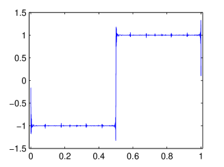
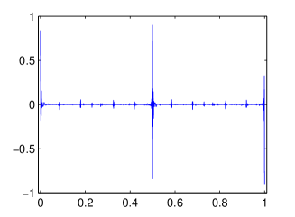
Figure 12: Left: the reconstruction based on finite-dimensional technique (4.13). Right: the error of the reconstruction.

• In the first example, we investigate what happens if we actually have a function

  $$f=\sum^{N}_{j=1}\tilde{\beta}_{j}\varphi_{j},$$

  for some $N\in\mathbb{N}$ that is a finite sum of step functions (recall that this was the first assumption leading up to the inverse crime). In particular, we choose $f=-\chi_{[0,1/2)}+\chi_{[1/2,1)},$ which is precisely the Haar wavelet. In Figure 12 we display the reconstruction obtained from solving (4.10), where $V_{\mathrm{dw}}$ is based on the Haar wavelet. Since $f$ is sparse in the Haar wavelet basis, we may have hoped to recover it exactly. However, this is by no means the case, and as we see, the reconstruction is polluted by many oscillations.

  To explain this, we can appeal to the previous discussion. Consider the vector

  $$x=U_{\mathrm{df}}^{-1}P_{N}\hat{f},$$

  which, as discussed above, is the vector of pointwise evaluation of the truncated Fourier series $f_{N}$. Hence

  $$\tilde{x}=V_{\mathrm{dw}}x$$

  is a vector of (approximations to the) Haar wavelet coefficients of $f_{N}$. Since the truncated Fourier series of $f$ is an oscillatory function (it suffers from the Gibbs phenomenon), this vector is not sparse and we consequently do not recover $f$ exactly. Note that this is also the cause of the oscillatory artefacts seen in the reconstruction in Figure 12.

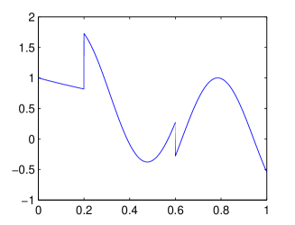
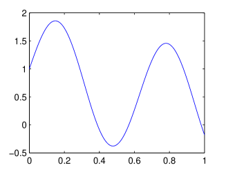
Figure 13: Left: the piecewise smooth test function $f_{1}$. Right: the smooth test function $f_{2}$

• In the second example, we first further illustrate the artefacts that arise from solving (4.13), and then show how the infinite-dimensional CS approach (4.10) yields a much improved result. To do so, we consider the piecewise smooth function

  $$f_{1}(t)=e^{-t}\chi_{[0,0.6)}(t)+\sin(10t)\chi_{[0.2,1)}(t),\qquad t\in[0,1],$$

  (see left panel of Figure 13). In Figure 14 the reconstructions using firstly periodized, and secondly boundary, Daubechies 6 (DB6) wavelets are displayed. Note that the infinite-dimensional compressed sensing implementation always yields a superior reconstruction.

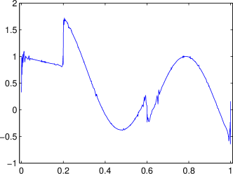
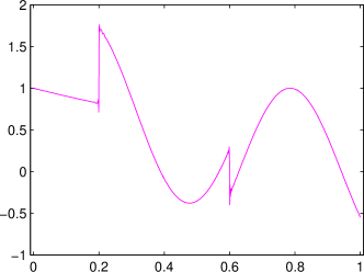
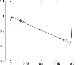
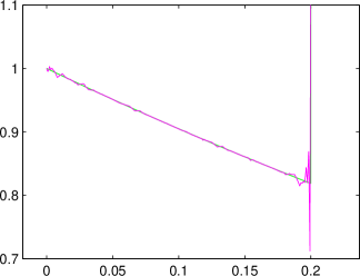
  Figure 14: Upper left: reconstruction obtained from (4.13) using periodized DB6 wavelets. Lower left: zoomed reconstruction from (4.13) using boundary DB6 wavelets. Upper right: reconstruction from (4.10) using boundary DB6 wavelets. Lower right: zoomed reconstruction from (4.10) using boundary DB6 wavelets.

• In this third example, we demonstrate the most serious impact of the crimes by considering the smooth test function

  $$f_{2}(t)=e^{-t}\chi_{[0,1)}(t)+\sin(10t)\chi_{[0,1)}(t),\qquad t\in[0,1],$$

  (see right panel of Figure 13). The left panels of Figure 15 show the reconstruction errors resulting from solving (4.13) with periodized and boundary DB6 wavelets. The right panels show the corresponding results for the infinite-dimensional CS approach (4.10) using boundary DB6 wavelets and orthonormal Legendre polynomials. Clearly the finite-dimensional approach gives highly substandard reconstructions in comparison to the infinite-dimensional approach. Once more, this is easy to explain. The finite-dimensional approach yields a wavelet approximation to the truncated Fourier series $f_{N}$ of $f$. However, $f_{N}$ converges extremely slowly to $f$ (since $f$ is smooth, but not periodic), and this leads to the large errors displayed in the left panels. Conversely, since $f$ is a smooth function, the truncated wavelet expansion with the boundary wavelets converges much faster than the Fourier series [mallat09wavelet], and the convergence is even better when using Legendre polynomial expansions. The infinite-dimensional implementation (4.10) correctly exploits these properties in order to obtain superior reconstructions. For an infinite-dimensional implementation of compressed sensing in MRI see [PruessmannUnserMRIFast].

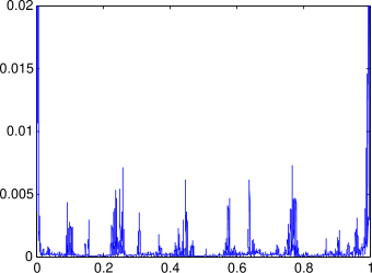
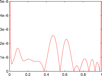
Figure 15: Left: errors for the reconstructions obtained from (4.13) using periodized (top) and boundary (bottom) DB6 wavelets. Right: errors for the reconstruction obtained from (4.10) using boundary DB6 wavelets (top) and Legendre polynomials (bottom).

The purpose of the remainder of this paper is to explain the success of the infinite-dimensional CS approach (4.10) as seen in these examples. As mentioned, in order to do this we are required to discard the three standard principles of finite-dimensional CS in favour of three new principles: asymptotic sparsity, asymptotic incoherence and multilevel random subsampling. We now introduce these new concepts. The new theory is presented in §4.4–4.7.

4.3 Asymptotic sparsity in levels

$\begin{array}[]{cc}\includegraphics[width=199.16928pt]{Anders-Ben_coef_per_DB4}&\includegraphics[width=199.16928pt]{Anders-Ben_coef_boundary_DB4}\end{array}$

Figure 16: Left: scaled periodic DB6 wavelet coefficients $\{\sqrt{j}|\beta_{j}|\}_{j\in\mathbb{N}}$ of the piecewise smooth test function $f_{1}$. Right: scaled boundary DB6 wavelet coefficients. Note that boundary wavelets yield better sparsity.

In order to introduce a new notion of sparsity in infinite dimensions, let us commence with a series of observations. First, in infinite dimensions, one cannot allow $s$ nonzero coefficients of a sparse vector $\beta\in\ell^{2}(\mathbb{N})$ to have completely arbitrary locations in the infinite range $1,2,\ldots$. In particular, one must place an upper bound on the bandwidth $M$, i.e. the smallest integer such that

$$\mathrm{supp}(\beta)\subseteq\{1,\ldots,M\},$$

of the nonzero coefficients. The reason for this can be traced back to GS. Consider the case of Fourier sampling with a wavelet sparsity basis. A large value of $M$ would necessarily require a sampling strategy that took (possibly sub-) samples at frequencies within some correspondingly large bandwidth $N$, where $N$ is related to $M$ through some property similar to the stable sampling rate. If $N$ were not taken sufficiently large, there would be no way to recover the fine scale wavelet coefficients from only low frequency Fourier measurements. Thus, at the very least, we must consider classes of signals that are not merely $s$-sparse, in the sense that they have only $s$ nonzero entries, but actually $(s,M)$-sparse, i.e. the $s$ nonzero entries lie in some given bandwidth $M$.

Our second observation pertains to the nature of the sparsity. Let $\{\varphi_{j}\}_{j\in\mathbb{N}}$ be a given orthonormal basis, and suppose that $f=\sum_{j\in\mathbb{N}}\beta_{j}\varphi_{j}$ is $(s,M)$-compressible in this basis, i.e. it is well approximated by an $(s,M)$-sparse signal. Then we may ask the following question: for ‘real-life’ signals $f$ is there any pattern to the sparsity? To answer this, let us note first that since $\{\varphi_{j}\}_{j\in\mathbb{N}}$ is an orthonormal basis, the coefficient vector $\beta=\{\beta_{j}\}_{j\in\mathbb{N}}\in\ell^{2}(\mathbb{N})$. In particular, $\beta_{j}\rightarrow 0$ as $j\rightarrow\infty$. Hence the most significant coefficients naturally correspond to smaller indices $j$. Thus there will always be a sufficiently large value of the bandwidth $M$ for which the ‘important’ coefficients of the signal $f$ lie in the range $\{1,\ldots,M\}$.

This gives an indication that the sparsity of a typical signal increases as the bandwidth $M\rightarrow\infty$. To see this more clearly, let us now investigate the important case of a wavelet basis $\{\varphi_{j}\}_{j\in\mathbb{N}}$ in more detail. It is often stated that typical signals and images are compressible in wavelet bases. But is there any structure to this sparsity? Recall that associated to such a basis, there is a natural decomposition of $\mathbb{N}$ into finite subsets according to different scales, i.e.

$$\mathbb{N}=\bigcup_{k\in\mathbb{N}}\{M_{k-1}+1,\ldots,M_{k}\},$$

where $0=M_{0}<M_{1}<M_{2}<\ldots$ and $\{M_{k-1}+1,\ldots,M_{k}\}$ is the set of indices corresponding to the $k^{\mathrm{th}}$ scale. Note that, for wavelets, $M_{k}-M_{k-1}=\mathcal{O}\left(2^{k}\right)$ in the 1D case and $M_{k}-M_{k-1}=\mathcal{O}\left(4^{k}\right)$ in the 2D case. Suppose now that $\epsilon\in(0,1]$ is given, and let

$$s_{k}:=s_{k}(\epsilon)=\min\Big{\{}K:\Big{\|}\sum_{i=1}^{K}\beta_{\pi(i)}\varphi_{\pi(i)}\Big{\|}\geq\epsilon\,\Big{\|}\sum_{i=M_{k-1}+1}^{M_{k}}\beta_{j}\varphi_{j}\Big{\|}\,\Big{\}},$$ (4.14)

in order words, $s_{k}$ is the effective sparsity at the $k^{\mathrm{th}}$ scale. Here $\pi:\{1,\ldots,M_{k}-M_{k-1}\}\rightarrow\{M_{k-1}+1,\ldots,M_{k}\}$ is a bijection such that $|\beta_{\pi(i)}|\geq|\beta_{\pi(i+1)}|.$ Note that this definition makes sense even if $\{\varphi_{j}\}_{j\in\mathbb{N}}$ is a tight frame. If $\{\varphi_{j}\}_{j\in\mathbb{N}}$ is an orthonormal basis then we have that

$$s_{k}=\min\Big{\{}K:\Big{(}\sum_{i=1}^{K}{|\beta_{\pi(i)}|}^{2}\Big{)}^{\!1/2}\geq\epsilon\,{\big{\|}P_{M_{k}}^{M_{k-1}}\beta\big{\|}}\Big{\}},$$ (4.15)

where the projection $P_{M_{k}}^{M_{k-1}}$ is defined as

$$P_{M_{k}}^{M_{k-1}}\beta=\{0,\ldots,0,\beta_{M_{k-1}+1},\ldots,\beta_{M_{k}},0,\ldots\}.$$ (4.16)

Sparsity of a signal $f$ in a wavelet basis thus means that for a given $r\in\mathbb{N}$, the ratio $s/M_{r}\ll 1$, where $s=s_{1}+\ldots+s_{r}$ is the total effective sparsity of $f$ and $M=M_{r}$. However, this is not only the case in practice, but moreover, one also has asymptotic sparsity, i.e.

$$s_{k}/(M_{k}-M_{k-1})\rightarrow 0,$$

rapidly as $k\rightarrow\infty$, for every $\epsilon\in(0,1]$. In other words, typical signals and images are much more sparse at fine scales (large $k$) than at coarse scales (small $k$). This phenomenon is heuristically displayed in Figure 16 and quantified in Figure 17. In particular, in Figure 17 each vertical cross-section corresponds to a particular value of $\epsilon$, and $s_{k}/(M_{k}-M_{k-1})$ is where the (coloured) $k^{\mathrm{th}}$ function intersects the vertical line (the wavelet used is DB8).

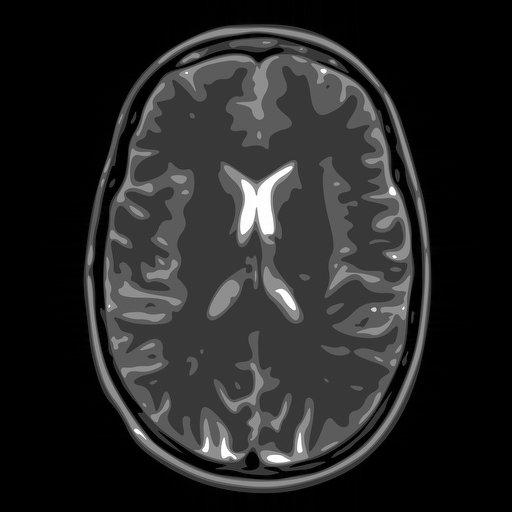
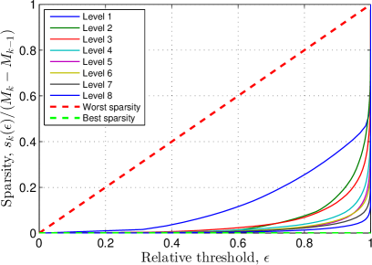
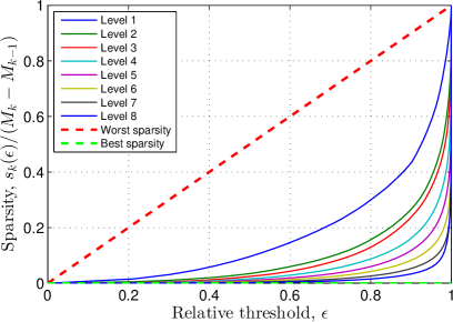
Figure 17: Relative sparsity of Daubechies 8 wavelet coefficients on dyadic levels of the GLPU phantom [GLPU] and a real-world image. $s_{k}(\epsilon)$ is defined in (4.15). The levels here correspond to the wavelet scales. Each curve shows the relative sparsity at level $k$ as a function of $\epsilon$, i.e. the minimum fraction of largest coefficients in the $k^{\mathrm{th}}$ level whose $\ell^{2}$ norm is larger than $\epsilon$-percent of the $\ell^{2}$ norm of all coefficients in the $k^{\mathrm{th}}$ level.

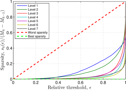
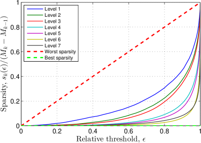
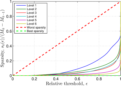
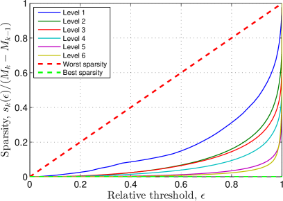
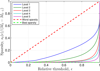
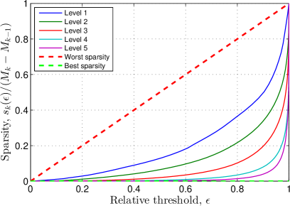
Figure 18: Relative sparsity as in Figure 17 of frame coefficients other than wavelets, all showing asymptotic sparsity. Top: Curvelets. Middle: Contourlets. Bottom: Shearlets. The different levels depicted correspond to the decomposition scales of each frame.

This observation should come as little surprise. It is well-known that piecewise smooth signals or images have wavelet coefficients that at fine scales are vanishingly small when their supports are contained within smooth regions of $f$ and are only large when their supports intersect its discontinuities. Since the number of discontinuities is fixed, this translates into increasing sparsity at finer scales, and this is precisely what we see in Figure 17.

To summarize, for images and signals encountered in practice, it is always the case that their wavelet coefficients possess asymptotic sparsity. Note that this conclusion does not change fundamentally if we replace wavelets by other related approximation systems, such as curvelets [candes2004new], contourlets [Vetterli] or shearlets [Gitta3], which is what we observe in Figure 18.

We are now in a position to formally define the concept of asymptotic sparsity in levels:

Definition 4.4.

For $r\in\mathbb{N}$ let $\mathbf{M}=(M_{1},\ldots,M_{r})\in\mathbb{N}^{r}$ with $1\leq M_{1}<\ldots<M_{r}$ and $\mathbf{s}=(s_{1},\ldots,s_{r})\in\mathbb{N}^{r}$, with $s_{k}\leq M_{k}-M_{k-1}$, $k=1,\ldots,r$, where $M_{0}=0$. We say that $\beta\in l^{2}(\mathbb{N})$ is $(\mathbf{s},\mathbf{M})$-sparse if, for each $k=1,\ldots,r$,

$$\Delta_{k}:=\mathrm{supp}(\beta)\cap\{M_{k-1}+1,\ldots,M_{k}\},$$

satisfies $|\Delta_{k}|\leq s_{k}$. We denote the set of $(\mathbf{s},\mathbf{M})$-sparse vectors by $\Sigma_{\mathbf{s},\mathbf{M}}$.

Definition 4.5.

Let $f=\sum_{j\in\mathbb{N}}\beta_{j}\varphi_{j}\in\mathcal{H}$, where $\beta=(\beta_{j})_{j\in\mathbb{N}}\in l^{1}(\mathbb{N})$. We say that $f$ is $(\mathbf{s},\mathbf{M})$-compressible with respect to $\{\varphi_{j}\}_{j\in\mathbb{N}}$ if $\sigma_{\mathbf{s},\mathbf{M}}(f)$ is small, where

$$\sigma_{\mathbf{s},\mathbf{M}}(f):=\min_{\eta\in\Sigma_{\mathbf{s},\mathbf{M}}}\|\beta-\eta\|_{l^{1}}.$$ (4.17)

Note that the levels here do not necessarily correspond to wavelet scales, although, as discussed above, this is obviously an important case. We note also that these definitions are natural generalizations of $(s,M)$-sparsity and compressibility.

4.3.1 Sparsity is too crude

Having introduced the new concept of asymptotic sparsity, it is important to ask whether it is actually necessary. Indeed, could it be the case that standard sparsity, or more precisely $(s,M)$-sparsity, adequately explains the types of reconstructions seen in the examples in the previous section without having to resort to a more complicated level-based sparsity?

As it transpires, onne can show that this is not the case by means of a simple numerical experiment. Suppose that one were able to provide a theoretical recovery guarantee that related the total number of samples $m$ to the sparsity $s$ (i.e. an estimate similar to the finite-dimensional result (4.4)). The sparsity of a signal is unchanged by random permutation of its coefficients. Thus, in order to test whether the relevance of such recovery guarantees to actual experiments, one can perform the following test. First one applies CS to an image with a certain subsampling pattern (i.e. a certain index set $\Omega$). This is shown in Figure 19. Next one takes the original image, computes its wavelet coefficients, forms a new image by reversing the order of the wavelet coefficients, and then runs the same reconstruction algorithm (with, importantly, the same subsampling pattern) on this new image, giving a new set of reconstructed coefficients. Finally, one reverses the order of the computed coefficients to give the final reconstruction. The result of this process is shown in Figure 20. Had sparsity been the correct signal model to explain the recovery results for the original image, then we would have seen a similar reconstruction in Figure 20 since the sparsity of the image is unchanged by permutations. However, this recovered image is clearly drastically worse. Thus we conclude that sparsity is indeed too crude to explain the reconstructions seen in practice.

This fact is perhaps not surprising. Suppose an image had $s$ nonzero Haar wavelet coefficients, or in other words, it is piecewise constant with a number of jumps proportional to $s$. It is known that in order to recover a piecewise constant function stably, one must take Fourier samples in a range where the maximal frequency is proportional to the reciprocal of the minimal distance between consecutive jumps [CandesSuperresolution]. Now suppose that the $s$ nonzero coefficients occur at the $s$ lowest indices. Then this minimal distance is rather large. However, if those $s$ coefficients are permuted to a fine wavelet scale, then this minimal distance becomes substantially smaller. Thus, one cannot expect to reconstruct the latter function from the sampling pattern used for the former, even though the sparsity is identical.

Of course, asymptotic sparsity in levels does not allow such permutations, since doing so would change the parameter $\mathbf{s}$. In this sense, it is a more realistic signal model to analyze the true reconstruction quality achieved in practical CS simulations.

4.3.2 Sparsity-based theory of compressed sensing in infinite dimensions

Despite having argued why sparsity is too crude a signal model in infinite dimensions, in order to explain the next principle of asymptotic incoherence it is useful to recall an earlier theoretical result on infinite-dimensional CS based on sparsity. Such a theory was introduced in [BAACHGSCS], and in particular, the following result was proven. Suppose that

$$\mathrm{supp}(\beta)=\{j:\beta_{j}\neq 0\}\subseteq\{1,\ldots,M\},\qquad|\mathrm{supp}(\beta)|=s,$$

for $s,M\in\mathbb{N}$ and let $m,N\in\mathbb{N}$ be chosen so that the so-called weak balancing property holds (see Definition 4.10). Suppose also that $\Omega\subseteq\{1,\ldots,N\}$ is chosen uniformly at random with $|\Omega|=m$. Then $f=\sum_{j\in\mathbb{N}}\beta_{j}\varphi_{j}$ is recovered exactly from (4.9), provided

$$m\gtrsim\mu(A)\cdot N\cdot s\cdot(1+\log(\epsilon^{-1}))\cdot\log(m^{-1}MN\sqrt{s}).$$ (4.18)

Note that this result is similar to the corresponding finite-dimensional estimate (4.4), and indeed, the latter is a corollary of (4.18).

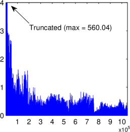
Figure 19: Left and Middle: Reconstruction of the image from 10% of its Fourier coefficients at $1024\!\times\!1024$ resolution using two sub-sampling patterns. Right: DB8 wavelet coefficients of the original image.

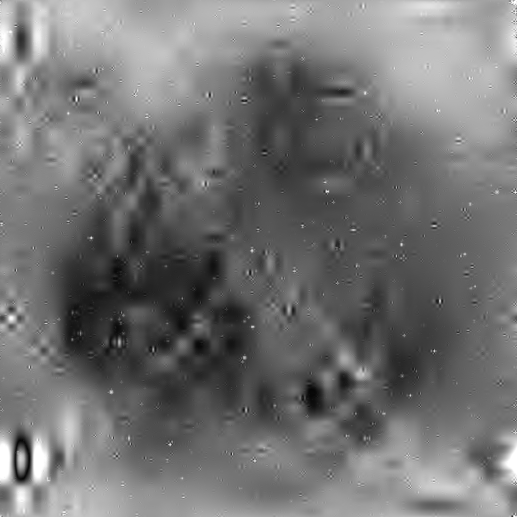
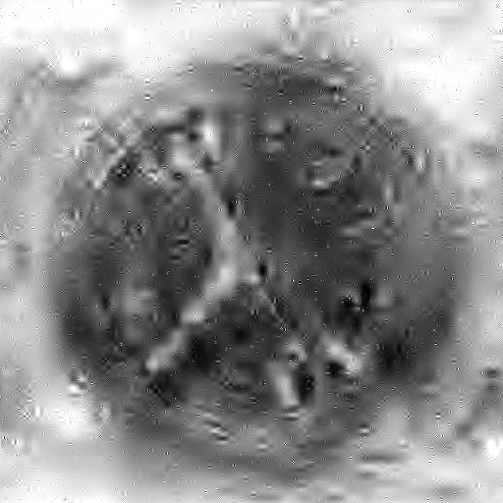
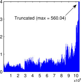
Figure 20: Left and Middle: Reconstruction of the image formed by reversing its wavelet coefficients, from 10% of its Fourier coefficients at $1024\!\times\!1024$ resolution using the same two sub-sampling patterns used in Figure 19. Right: Reversed DB8 wavelet coefficients of the original image.

4.4 Asymptotic incoherence

We now turn our attention to the second concept of asymptotic incoherence. To introduce this, let us compare the finite-dimensional CS estimate (4.4) to (4.18). Although superficially these results are very similar, there is a key difference between them. In (4.18), the infinite matrix $A$ is fixed independently of the sampling bandwidth $N$, whereas in (4.4) the $N\times N$ matrix $A$ usually changes with $N$. In finite dimensions it is therefore possible to construct matrices $A$ for which $\mu(A)=\mathcal{O}\left(N^{-1}\right)$ (e.g. the DFT matrix), and in such cases one guarantees through (4.4) exact recovery of all $s$-sparse vectors using roughly $s\log N$ measurements.

In infinite dimensions, the situation changes completely. For a given infinite matrix $A$ one can only guarantee such near-optimal recovery for sufficiently small $N$: specifically, $N\lesssim 1/\mu(A)$. Since $N$ is usually at least the size of the signal bandwidth $M$, this means that there will be infinitely many $(s,M)$-sparse signals (specifically those with bandwidth larger than this threshold) for which exact recovery is not possible with near-optimal numbers (i.e. proportional to $s$ up to log factors) of measurements.

Fortunately, the situation is not completely hopeless, since it is indeed possible given an arbitrarily small $\mu^{*}>0$ to design an infinite matrix $A$ with a coherence $\mu(A)\leq\mu^{*}$. However, it is rare for such a matrix to correspond to the physical sampling system such as those found in MRI or X-ray tomography. Indeed, the usual formulations of these problems result in systems with large coherences. For instance, in the examples of §4.2.5, which assume Fourier sampling with either wavelet or polynomial sparsity, the coherence $\mu(A)\approx 1$ [AHPRBreaking]. Thus, for any realistic bandwidth $M$, no substantial subsampling is possible according to (4.18). This is sometimes referred to as the coherence barrier.

On the face of it, this statement flies in the face of the good numerical recovery results seen in §4.2.5. There is no contradiction here, however. In particular, the results in §4.2.5 were obtained by choosing the sampling set $\Omega$ according to (4.12), as opposed to uniformly at random, which is the setting of (4.18). The reason for the success of the former in comparison to the latter is due to the second key principle we now introduce: namely, the so-called asymptotic incoherence of the Fourier and wavelet (or polynomial) bases.

Let $P_{N}\in\mathcal{B}(l^{2}(\mathbb{N}))$ be the projection operator onto $\mathrm{span}\{e_{j}:j=1,\ldots,N\}$, where $\{e_{j}\}_{j\in\mathbb{N}}$ is the canonical basis for $l^{2}(\mathbb{N})$. The abstract definition of asymptotic incoherence is as follows:

Definition 4.6.

Let $A\in\mathcal{B}(l^{2}(\mathbb{N}))$ be an isometry. Then $A$ is asymptotically incoherent if

$$\mu(P^{\perp}_{N}A),\ \mu(AP^{\perp}_{N})\rightarrow 0,\quad N\rightarrow\infty.$$ (4.19)

Equivalently, $A$ is asymptotically incoherent if the coherence of the infinite matrices formed by replacing either the first $N$ rows or columns of $A$ by zeros tends to zero as $N\rightarrow\infty$. Note that it is not always the case that two orthonormal bases $\{\psi_{j}\}_{j\in\mathbb{N}}$ and $\{\varphi_{j}\}_{j\in\mathbb{N}}$ give rise to an asymptotically incoherent matrix $A$ (e.g. in the case $\psi_{j}=\varphi_{j}$, $\forall j$, one has $\mu(P^{\perp}_{N}A)=\mu(AP^{\perp}_{N})=1$, $\forall N$). However, asymptotic incoherence is indeed witnessed in the following important situations:

• Let $\{\psi_{j}\}_{j\in\mathbb{N}}$ be the Fourier basis on $[0,1]$ and $\{\varphi_{j}\}_{j\in\mathbb{N}}$ be any orthonormal basis of compactly supported wavelets associated with a multiresolution analysis (MRA). Then $\mu(P^{\perp}_{N}A),\ \mu(AP^{\perp}_{N})=\mathcal{O}\left(N^{-1}\right)$ as $N\rightarrow\infty$ [AHPRBreaking, Thm. 3.2].

• Let $\{\psi_{j}\}_{j\in\mathbb{N}}$ be the Fourier basis on $[0,1]$ and $\{\varphi_{j}\}_{j\in\mathbb{N}}$ be the orthonormal basis of Legendre polynomials. Then $\mu(P^{\perp}_{N}A),\ \mu(AP^{\perp}_{N})=\mathcal{O}\left(N^{-2/3}\right)$ as $N\rightarrow\infty$ [Jones2013Incoherence].

It is known that $\mu(P^{\perp}_{N}A)$ and $\mu(AP^{\perp}_{N})$ cannot both decrease faster than $N^{-1}$ [Jones2013Incoherence]. Hence the combination of Fourier and wavelets possesses so-called perfect asymptotic incoherence.

An illustration of asymptotic incoherence for the two examples listed above is given in Figure 21. Note that the large entries of the matrix $A$ in both cases are located near the low frequencies in the sampling and sparsity bases (recall that we index the Fourier basis over $\mathbb{Z}$ as opposed to $\mathbb{N}$), and the entries get progressively smaller as one moves away either vertically or horizontally.

Figure 21: Plots of the absolute values of the entries of the matrix $A$ for corresponding to Fourier sampling with Haar wavelets (left) and Legendre polynomials (right). Lighter regions correspond to larger values and darker regions to smaller values.

4.5 Multilevel random subsampling

Suppose $A$ is an asymptotic incoherent, yet globally coherent, matrix. We are interested in subsampling its rows so as to take advantage of the asymptotic sparsity in the signal to be recovered. This question is, how does one best do this? Clearly one cannot subsample the first $N$ rows uniformly at random, since the high global coherence will prohibit good recovery. However, the asymptotic incoherence of $A$ means that its high coherence is concentrated only in its first few rows. Thus, to ensure good recovery we need to fully sample these rows, whereas in the remaining rows, where the coherence is smaller, we are free to subsample.

Let $N_{1},N,m\in\mathbb{N}$ be given. This argument now leads us to consider an index set $\Omega$ of the form $\Omega=\Omega_{1}\cup\Omega_{2}$, where $\Omega_{1}=\{1,\ldots,N_{1}\}$, and $\Omega_{2}\subseteq\{N_{1}+1,\ldots,N\}$ is chosen uniformly at random with $|\Omega_{2}|=m$. We refer to this as a two-level sampling scheme. Note that the index set (4.12) used in the examples in §4.2.5 has precisely this form. As we shall show later, the amount of subsampling possible (i.e. the parameter $m$) in the region corresponding to $\Omega_{2}$ will depend solely on the sparsity of the signal and coherence $\mu(P^{\perp}_{N_{1}}A)$, which is of course much smaller than the global coherence $\mu(A)$ since $A$ is asymptotically incoherent.

The two-level scheme represents the simplest type of subsampling map for asymptotically incoherent matrices. There is no reason, however, to restrict our attention to just two levels (full and subsampled). In general, we may consider multilevel schemes, defined as follows:

Definition 4.7.

Let $r\in\mathbb{N}$, $\mathbf{N}=(N_{1},\ldots,N_{r})\in\mathbb{N}^{r}$ with $1\leq N_{1}<\ldots<N_{r}$, $\mathbf{m}=(m_{1},\ldots,m_{r})\in\mathbb{N}^{r}$, with $m_{k}\leq N_{k}-N_{k-1}$, $k=1,\ldots,r$, and suppose that

$$\Omega_{k}\subseteq\{N_{k-1}+1,\ldots,N_{k}\},\quad|\Omega_{k}|=m_{k},\quad k=1,\ldots,r,$$

are chosen uniformly at random, where $N_{0}=0$. We refer to the set

$$\Omega=\Omega_{\mathbf{N},\mathbf{m}}:=\Omega_{1}\cup\ldots\cup\Omega_{r}.$$

as an $(\mathbf{N},\mathbf{m})$-multilevel sampling scheme.

The same guiding principle applies as in the two-level case. In the region of highest coherence, i.e. $\Omega_{1}$, we take more measurements, and as coherences decreases, i.e. as the level number $k$ increases, we take progressively fewer. Note that our introduction of multilevel schemes is not just for the purposes of mathematical intricacy: in practice, they are often more effective than two-level schemes.

4.6 Asymptotic sparsity, asymptotic incoherence and multilevel random subsampling in finite dimensions

Somewhat surprisingly, these three new principles, whilst motivated by infinite-dimensional considerations are actually relevant in finite dimensions as well. Indeed, digital signals and images are not just sparse in discrete wavelet bases, but, much like their analog analogues are in fact asymptotically sparse in levels. And moreover, if one considers the discrete model of Fourier sampling, where the sampling is modelled via the DFT, then one finds exactly the same phenomenon of asymptotic incoherence. Thus, multilevel sampling should also be applied in this case. Note that the theory we shall develop below is equally applicable in this setting, and finite-dimensional results are corollaries of the infinite-dimensional theorems.

The reason for this connection is that such finite-dimensional problems typically arise out of discretizations of infinite-dimensional problems. Thus it should come as little surprise that asymptotic sparsity in wavelets, i.e. orthogonal bases over the continuum, and asymptotic incoherence with the continuous Fourier transform should be transferred over when discretizing.

To clarify this, let make this connection explicit for the discrete CS model (4.7). If we embed the matrix $U_{\mathrm{df}}V^{-1}_{\mathrm{dw}}\in\mathbb{C}^{n\times n}$ in the natural way into $\mathcal{B}(l^{2}(\mathbb{N}))$, then by using the properties of the discrete wavelet transform, convergence of Fourier series and the Lebesgue dominated convergence theorem, we get

$$\underset{n\rightarrow\infty}{\text{WOT-lim \,}}U_{\mathrm{df}}V^{-1}_{\mathrm{dw}}=A,$$ (4.20)

where

$$A=\left(\begin{array}[]{ccc}\left<\varphi_{1},\psi_{1}\right>&\left<\varphi_{2},\psi_{1}\right>&\cdots\\ \left<\varphi_{1},\psi_{2}\right>&\left<\varphi_{2},\psi_{2}\right>&\cdots\\ \vdots&\vdots&\ddots\end{array}\right),$$

the $\varphi_{j}$s are the wavelets used, the $\psi_{j}$ are the complex exponentials and WOT denotes the weak operator topology. Note that this is a very weak form of convergence (non-uniform convergence of the matrix elements), and as we have seen, this results in artefacts (some spectacularly bad) in the finite-dimensional CS. However, (4.20) gives a clear picture as to why we will also see asymptotic incoherence even in the finite-dimensional model, simply because it is a (poor) discretization of a fundamentally infinite-dimensional problem with the same property.

We remark also that, even if the artefacts resulting from the finite-dimensional approach (4.7) were tolerable in some application, in order to properly understand the reconstructions obtained, one still needs to argue (due to the fact that the data arises from the continuous model) via (4.20). Thus infinite-dimensional CS also provides the link between discrete CS and continuous data.

4.7 Theory

We are now ready to present our theory for CS based on asymptotic sparsity, asymptotic incoherence and multilevel random subsampling. Note that in realistic problems, signals are never exactly sparse (or asymptotically sparse), and their measurements are always contaminated by noise. Let $f=\sum_{j}\beta_{j}\varphi_{j}$ be a fixed signal, and let

$$y=P_{\Omega}\hat{f}+z=P_{\Omega}A\beta+z,$$

be its noisy measurements, where $z\in\mathrm{ran}(P_{\Omega})$ is a noise vector satisfying $\|z\|\leq\delta$ for some $\delta\geq 0$. In our theorems we shall consider the following problem:

$$\inf_{\eta\in\ell^{1}(\mathbb{N})}\|\eta\|_{\ell^{1}}\text{ subject to }\|P_{\Omega}A\eta-y\|\leq\delta.$$ (4.21)

Clearly the equality-constrained problem

$$\inf_{\eta\in\ell^{1}(\mathbb{N})}\|\eta\|_{\ell^{1}}\text{ subject to }P_{\Omega}A\eta=y,$$

is just a special case corresponding to $\delta=0$.

In order to state our theorems, we first require several definitions:

Definition 4.8.

Let $A\in\mathcal{B}(\ell^{2}(\mathbb{N}))$ be an isometry. Given $N\in\mathbb{N}$ we define

$$\mu_{N}=\mu(P^{\perp}_{N}A).$$

If $\mathbf{N}=(N_{1},\ldots,N_{r})\in\mathbb{N}^{r}$ and $\mathbf{M}=(M_{1},\ldots,M_{r})\in\mathbb{N}^{r}$ with $1\leq N_{1}<\ldots N_{r}$ and $1\leq M_{1}<\ldots<M_{r}$ we define the $(k,l)^{\mathrm{th}}$ local coherence of $A$ with respect to $\mathbf{N}$ and $\mathbf{M}$ by

$$\mu_{\mathbf{N},\mathbf{M}}(k,l) =\sqrt{\mu(P^{N_{k-1}}_{N_{k}}AP^{M_{l-1}}_{M_{l}})\cdot\mu(P^{N_{k-1}}_{N_{k}}A)},\quad k,l=1,\ldots,r,$$

where $N_{0}=M_{0}=0$ and $P^{N_{k-1}}_{N_{k}}$, $P^{M_{l-1}}_{M_{l}}$ are as in (4.16). Further, we let

$$\mu_{\mathbf{N},\mathbf{M}}(k,\infty) =\sqrt{\mu(P^{N_{k-1}}_{N_{k}}AP_{M_{r-1}}^{\perp})\cdot\mu(P^{N_{k-1}}_{N_{k}}A)},\quad k,l=1,\ldots,r,$$

Definition 4.9.

Let $A$ be an isometry of either $\mathbb{C}^{N\times N}$ or $\mathcal{B}(l^{2}(\mathbb{N}))$. For $\mathbf{N}=(N_{1},\ldots,N_{r})\in\mathbb{N}^{r}$, $\mathbf{M}=(M_{1},\ldots,M_{r})\in\mathbb{N}^{r}$ with $1\leq N_{1}<\ldots<N_{r}$ and $1\leq M_{1}<\ldots<M_{r}$, $\mathbf{s}=(s_{1},\ldots,s_{r})\in\mathbb{N}^{r}$ and $1\leq k\leq r$, let

$$S_{k}=S_{k}(\mathbf{N},\mathbf{M},\mathbf{s})=\max_{\eta\in\Theta}\|P_{N_{k}}^{N_{k-1}}A\eta\|^{2},$$

where $N_{0}=M_{0}=0$, the projection $P_{N_{k}}^{N_{k-1}}$ is defined in (4.16), and $\Theta$ is given by

$$\Theta=\{\eta:\|\eta\|_{\ell^{\infty}}\leq 1,|\mathrm{supp}(P_{M_{l}}^{M_{l-1}}\eta)|=s_{l},\,l=1,\ldots,r\}.$$

Definition 4.10.

Let $A\in\mathcal{B}(l^{2}(\mathbb{N}))$ be an isometry. Then $N\in\mathbb{N}$ and $K\geq 1$ satisfy the weak balancing property with respect to $A,$ $M\in\mathbb{N}$ and $s\in\mathbb{N}$ if

$$\begin{split}\|P_{M}A^{*}P_{N}AP_{M}-P_{M}\|_{\ell^{\infty}\rightarrow\ell^{\infty}}\leq\frac{1}{8}\left(\log_{2}^{1/2}\left(4\sqrt{s}KM\right)\right)^{-1},\end{split}$$ (4.22)

where ${\left\|\cdot\right\|}_{\ell^{\infty}\rightarrow\ell^{\infty}}$ is the norm on $\mathcal{B}(\ell^{\infty}(\mathbb{N}))$. We say that $N$ and $K$ satisfy the strong balancing property with respect to $A,$ $M$ and $s$ if (4.22) holds, as well as

$$\begin{split}\|P_{M}^{\perp}A^{*}P_{N}AP_{M}\|_{\ell^{\infty}\rightarrow\ell^{\infty}}\leq\frac{1}{8}.\end{split}$$ (4.23)

Note that the balancing property is the direct analogue of the stable sampling rate for infinite-dimensional CS. See Remark 4.7.2.

4.7.1 The finite-dimensional case

To avoid pathological cases we will assume from now on that the total sparsity $s\geq 3$. This is simply to make sure that $\log(s)\geq 1$.

We commence with the finite-dimensional case:

Theorem 4.11.

Let $A\in\mathbb{C}^{N\times N}$ be an isometry and $\beta\in\mathbb{C}^{N}$. Suppose that $\Omega=\Omega_{\mathbf{N},\mathbf{m}}$ is a multilevel sampling scheme, where $\mathbf{N}=(N_{1},\ldots,N_{r})\in\mathbb{N}^{r}$ and $\mathbf{m}=(m_{1},\ldots,m_{r})\in\mathbb{N}^{r}$. Let $(\mathbf{s},\mathbf{M})$, where $\mathbf{M}=(M_{1},\ldots,M_{r})\in\mathbb{N}^{r}$, $M_{1}<\ldots<M_{r}$, and $\mathbf{s}=(s_{1},\ldots,s_{r})\in\mathbb{N}^{r}$, be any pair such that the following holds: for $\epsilon>0$ and $1\leq k\leq r$,

$$1\gtrsim\frac{N_{k}-N_{k-1}}{m_{k}}\cdot(\log(\epsilon^{-1})+1)\cdot\left(\sum_{l=1}^{r}\mu_{\mathbf{N},\mathbf{M}}(k,l)\cdot s_{l}\right)\cdot\log\left(N\right),$$ (4.24)

where $s:=s_{1}+\ldots+s_{r}$ and

$$m_{k}\gtrsim\hat{m}_{k}\cdot(\log(\epsilon^{-1})+1)\cdot\log\left(N\right),$$

with $\hat{m}_{k}$ satisfying

$$1\gtrsim\sum_{k=1}^{r}\left(\frac{N_{k}-N_{k-1}}{\hat{m}_{k}}-1\right)\cdot\mu_{\mathbf{N},\mathbf{M}}(k,l)\cdot\tilde{s}_{k},\qquad\forall\,l=1,\ldots,r,$$ (4.25)

for all $\tilde{s}_{1},\ldots,\tilde{s}_{r}\in(0,\infty)$ such that

$$\tilde{s}_{1}+\ldots+\tilde{s}_{r}\leq s_{1}+\ldots+s_{r},\qquad\tilde{s}_{k}\leq S_{k}(\mathbf{N},\mathbf{M},\mathbf{s}).$$

Suppose that $\xi\in\ell^{1}(\mathbb{N})$ is a minimizer of (4.21). Then, with probability exceeding $1-s\epsilon$, we have that

$$\|\xi-\beta\|\leq C\cdot\left(\delta\cdot\sqrt{K}\cdot\left(1+L\cdot\sqrt{s}\right)+\sigma_{\mathbf{s},\mathbf{M}}(f)\right),$$ (4.26)

for some constant $C$, where $\sigma_{\mathbf{s},\mathbf{M}}(f)$ is as in (4.17), $L=1+\frac{\sqrt{\log_{2}\left(6\epsilon^{-1}\right)}}{\log_{2}(4KM\sqrt{s})}$ and $K=\max_{k=1,\ldots,r}\left\{\frac{N_{k}-N_{k-1}}{m_{k}}\right\}$. If $m_{k}=N_{k}-N_{k-1}$, $1\leq k\leq r$, then this holds with probability $1$.

4.7.2 The infinite-dimensional case

We shall discuss Theorem 4.11 in a moment, but let us first present the corresponding infinite-dimensional result. For this, we require the following notation:

$$\tilde{M}=\min\{i\in\mathbb{N}:\max_{k\geq i}\|P_{N}Ue_{k}\|\leq 1/(32K\sqrt{s})\}.$$

Here $K$ is defined below.

Theorem 4.12.

Let $A\in\mathcal{B}(\ell^{2}(\mathbb{N}))$ be an isometry and $\beta\in\ell^{1}(\mathbb{N})$. Suppose that $\Omega=\Omega_{\mathbf{N},\mathbf{m}}$ is a multilevel sampling scheme, where $\mathbf{N}=(N_{1},\ldots,N_{r})\in\mathbb{N}^{r}$ and $\mathbf{m}=(m_{1},\ldots,m_{r})\in\mathbb{N}^{r}$. Let $(\mathbf{s},\mathbf{M})$, where $\mathbf{M}=(M_{1},\ldots,M_{r})\in\mathbb{N}^{r}$, $M_{1}<\ldots<M_{r}$, and $\mathbf{s}=(s_{1},\ldots,s_{r})\in\mathbb{N}^{r}$, be any pair such that the following holds:

1. the parameters

   $$N:=N_{r},\quad K:=\max_{k=1,\ldots,r}\left\{\frac{N_{k}-N_{k-1}}{m_{k}}\right\},$$

   satisfy the strong balancing property with respect to $A$, $M:=M_{r}$ and $s:=s_{1}+\ldots+s_{r}$;

2. for $\epsilon>0$ and $1\leq k\leq r$,

   $$1\gtrsim\frac{N_{k}-N_{k-1}}{m_{k}}\cdot(\log(\epsilon^{-1})+1)\cdot\left(\sum_{l=1}^{r}\mu_{\mathbf{N},\mathbf{M}}(k,l)\cdot s_{l}\right)\cdot\log\left(K\tilde{M}\sqrt{s}\right),$$

   (with $\mu_{\mathbf{N},\mathbf{M}}(k,r)$ replaced by $\mu_{\mathbf{N},\mathbf{M}}(k,\infty)$) and

   $$m_{k}\gtrsim\hat{m}_{k}\cdot(\log(\epsilon^{-1})+1)\cdot\log\left(K\tilde{M}\sqrt{s}\right),$$

   where $\hat{m}_{k}$ satisfies (4.25).

Suppose that $\xi\in\ell^{1}(\mathbb{N})$ is a minimizer of (4.21). Then, with probability exceeding $1-s\epsilon$,

$$\|\xi-\beta\|\leq C\cdot\left(\delta\cdot\sqrt{K}\cdot\left(1+L\cdot\sqrt{s}\right)+\sigma_{\mathbf{s},\mathbf{M}}(f)\right),$$ (4.27)

for some constant $C$, where $\sigma_{\mathbf{s},\mathbf{M}}(f)$ is as in (4.17), and $L=C\cdot\left(1+\frac{\sqrt{\log_{2}\left(6\epsilon^{-1}\right)}}{\log_{2}(4KM\sqrt{s})}\right)$. If $m_{k}=N_{k}-N_{k-1}$ for $1\leq k\leq r$ then this holds with probability $1$.

This theorem and its finite-dimensional analogue give conditions on the number of measurements $m_{k}$ required in the $k^{\mathrm{th}}$ level in terms of the sparsity $\mathbf{s}$, the local coherences $\mu_{\mathbf{N},\mathbf{M}}(k,l)$ and the quantities $S_{k}(\mathbf{N},\mathbf{M},\mathbf{s})$ for exact recovery of $(\mathbf{s},\mathbf{M})$-compressible signals up to an error determined by firstly the noise $\delta$ and the $(\mathbf{s},\mathbf{M})$-term approximation error $\sigma_{\mathbf{s},\mathbf{M}}(f)$. Note that the estimates (4.26) and (4.27) are direct extensions of standard (i.e. one-level) CS results to the multilevel setting. We remark also that it is possible to provide some simpler results in the special case of two levels. See [AHPRBreaking] for details.

It is crucial to understand the various estimates in Theorems 4.11 and 4.12. We discuss this next. But, first we make the following remark on the role of the balancing property, which is the primary difference between the two results.

• The balancing property ensures that the truncated matrix $P_{N}AP_{M}$ is close to an isometry. Much like with the stable sampling rate in GS, this is necessary in order to ensure stability in the mapping between measurements and coefficients. Note that, also analogously to the stable sampling rate, the balancing property does indeed hold, provided $N$ is chosen sufficiently large in comparison to $M$. On the other hand, no balancing property is required in the finite-dimensional case since $P_{N}AP_{M}\equiv A$ is an isometry by assumption.

4.7.3 Sharpness of the estimates – the block-diagonal case

To interpret the theorems presented above, let us first consider the block-diagonal case. To this end, suppose that $\Omega=\Omega_{\mathbf{N},\mathbf{m}}$ is a multilevel sampling scheme, where $\mathbf{N}=(N_{1},\ldots,N_{r})\in\mathbb{N}^{r}$ and $\mathbf{m}=(m_{1},\ldots,m_{r})\in\mathbb{N}^{r}$. Let $(\mathbf{s},\mathbf{M})$, where $\mathbf{M}=(M_{1},\ldots,M_{r})\in\mathbb{N}^{r}$, and suppose for simplicity that $\mathbf{M}=\mathbf{N}$. Consider the block-diagonal matrix

$$\mathbb{C}^{N\times N}\ni A=\bigoplus_{k=1}^{r}A_{k},\qquad A_{k}\in\mathbb{C}^{(N_{k}-N_{k-1})\times(N_{k}-N_{k-1})},\quad A_{k}^{*}A_{k}=I,$$

where $N_{0}=0$. Note that in this setting we have

$$S_{k}=s_{k},\qquad\mu_{\mathbf{N},\mathbf{M}}(k,l)=0,\quad k\neq l,$$

in Theorem 4.11. Also, since $\mu(\mathbf{N},\mathbf{M})(k,k)=\mu(A_{k})$, equations (4.24) and (4.25) reduce to

$$1\gtrsim\frac{N_{k}-N_{k-1}}{m_{k}}\cdot\left(\log(\epsilon^{-1})+1\right)\cdot\mu(A_{k})\cdot s_{k}\cdot\log N,$$

and

$$1\gtrsim\left(\frac{N_{k}-N_{k-1}}{\hat{m}_{k}}-1\right)\cdot\mu(A_{k})\cdot s_{k}.$$

In particular, it suffices to take

$$m_{k}\gtrsim(N_{k}-N_{k-1})\cdot\left(\log(\epsilon^{-1})+1\right)\cdot\mu(A_{k})\cdot s_{k}\cdot\log N,\quad 1\leq k\leq r.$$ (4.28)

This is as one expects: the number of measurements in the $k^{\mathrm{th}}$ level depends on the size of the level multiplied by the asymptotic incoherence and the sparsity in that level. Note that this result recovers the standard one-level results in finite dimensions [Candes_Plan, BAACHGSCS] up to the $1-s\epsilon$ bound on the probability. In particular, the typical bound would be $1-\epsilon$. The question as to whether or not this $s$ can be removed in the multilevel setting is open, although such a result would be more of a cosmetic improvement.

4.7.4 Sharpness of the estimates – the non-block diagonal case

The previous argument demonstrated that Theorem 4.11 is sharp, up to the probability term, in the sense that it reduces to the usual estimate (4.28) for block-diagonal matrices. A key step in showing this is noting that the quantities $S_{k}$ reduce to the sparsities $s_{k}$ in the block-diagonal case. Unfortunately, this is not true in the general setting. Note that one has the upper bound

$$S_{k}\leq s=s_{1}+\ldots+s_{r},$$

however in general there is usually interference between different sparsity levels, which means that $S_{k}$ need not have anything to do with $s_{k}$, or can indeed be proportional to the total sparsity $s$.

On the face of it, this may seem an undesirable aspect of the theorems, since $S_{k}$ may be significantly larger than $s_{k}$, and thus the estimate on the number of measurements $m_{k}$ required in the $k^{\mathrm{th}}$ level may also be much larger than the corresponding sparsity $s_{k}$. Could it therefore be that the $S_{k}$s are an unfortunate artefact of the proof? As we now show by example, this is not the case.

To do this, we consider the following setting. Let $N=rn$ for some $n\in\mathbb{N}$ and $\mathbf{N}=\mathbf{M}=(n,2n,\ldots,rn)$. Let $W\in\mathbb{C}^{n\times n}$ and $V\in\mathbb{C}^{r\times r}$ be isometries and consider the matrix

$$A=V\otimes W,$$

where $\otimes$ is the usual Kronecker product. Note that $A\in\mathbb{C}^{N\times N}$ is also an isometry. Now suppose that $\beta=(\beta_{1},\ldots,\beta_{r})\in\mathbb{C}^{N}$ is an $(\mathbf{s},\mathbf{M})$-sparse vector, where each $\beta_{k}\in\mathbb{C}^{n}$ is $s_{k}$-sparse. Then

$$A\beta=y,\quad y=(y_{1},\ldots,y_{r}),\ y_{k}=Wz_{k},\ z_{k}=\sum^{r}_{l=1}v_{kl}\beta_{l}.$$

Hence the problem of recovering $\beta$ from measurements $y$ with an $(\mathbf{N},\mathbf{m})$-multilevel strategy decouples into $r$ problems of recovering the vector $z_{k}$ from the measurements $y_{k}=Wz_{k}$, $k=1,\ldots,r$. Let $\hat{s}_{k}$ denote the sparsity of $z_{k}$. Since the coherence provides an information-theoretic limit [Candes_Plan], one requires at least

$$m_{k}\gtrsim n\cdot\mu(W)\cdot\hat{s}_{k}\cdot\log n,\quad 1\leq k\leq r.$$ (4.29)

measurements at level $k$ in order to recover each $z_{k}$, and therefore recover $\beta$, regardless of the reconstruction method used.

We now consider two examples of this setup:

• Let $\pi:\{1,\ldots,r\}\rightarrow\{1,\ldots,r\}$ be a permutation and let $V$ be the matrix with entries $v_{kl}=\delta_{l,\pi(k)}$. Since $z_{k}=\beta_{\pi(k)}$ in this case, the lower bound (4.29) reads

  $$m_{k}\gtrsim n\cdot\mu(W)\cdot s_{\pi(k)}\cdot\log n,\quad 1\leq k\leq r.$$ (4.30)

  Now consider Theorem 4.11 for this matrix. First, we note that a simple argument gives that

  $$S_{k}=s_{\pi(k)}.$$

  In particular, $S_{k}$ is completely unrelated to $s_{k}$, and may be much larger than $s_{k}$ if the permuted value $s_{\pi(k)}\gg s_{k}$. Substituting this into Theorem 4.11 and noting that $\mu_{\mathbf{N},\mathbf{M}}(k,l)=\mu(W)\delta_{l,\pi(k)}$ in this case, we arrive at the condition

  $$m_{k}\gtrsim r\cdot n\cdot\mu(W)\cdot\left(\log(\epsilon^{-1})+1\right)\cdot s_{\pi(k)}\cdot\log(nr).$$

  Up to factors in $r$, this is equivalent to (4.30).

• Now suppose that $V$ is the $r\times r$ DFT matrix. Suppose also that $s\leq n/r$ and that the $\beta_{k}$’s have disjoint support sets, i.e. $\mathrm{supp}(\beta_{k})\cap\mathrm{supp}(\beta_{l})=\emptyset$, $k\neq l$. Then by construction, each $z_{k}$ is $s$-sparse, and therefore the lower bound (4.29) reads

  $$m_{k}\gtrsim n\cdot\mu(W)\cdot s\cdot\log n,\quad 1\leq k\leq r.$$

  After a short argument, one finds that $s/r\leq S_{k}\leq s$ in this case. Hence, $S_{k}$ is typically much larger than $s_{k}$. Moreover, after noting that $\mu_{\mathbf{N},\mathbf{M}}(k,l)=\frac{1}{r}\mu(W)$, we find that Theorem 4.11 gives the condition

  $$m_{k}\gtrsim r\cdot n\cdot\mu(W)\cdot\left(\log(\epsilon^{-1})+1\right)\cdot s\cdot\log(nr).$$

  Thus, Theorem 4.11 obtains the lower bound in this case as well.

These examples show that the $S_{k}$s cannot be removed in general from any estimates on the number of measurements $m_{k}$. In this sense, the theorems are sharp. Moreover, they illustrate the phenomenon of interference, and in particular, that the number of samples $m_{k}$ required in each level need not be related to the sparsity $s_{k}$ in the corresponding level.

Fortunately, in the important case of wavelets and Fourier sampling, with the sparsity levels taken to be wavelet scales, one can show by analyzing the behaviour of the $S_{k}$s that if the sampling levels are designed appropriately, then the number of measurements $m_{k}$ in the $k^{\mathrm{th}}$ level is proportional to $s_{k}$ plus terms that decay exponentially in the level $l\neq k$. See [AHPRBreaking] for details. Thus, up to log factors, CS with multilevel sampling recovers wavelet coefficients using optimal numbers of measurements.

4.8 First consequence: the success of compressed sensing is resolution dependent

In the final three subsections, we discuss three main consequences of our theorems. To commence, we consider a rather intriguing phenomenon that occurs in the presence asymptotic sparsity and asymptotic incoherence: namely resolution dependence. We illustrate this via the following two examples.

256x256 Error: 16.06%
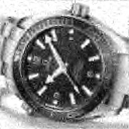
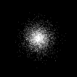
512x512 Error: 11.80%
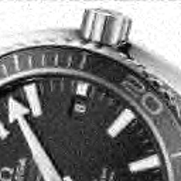
1024x1024 Error: 9.22%
2048x2048 Error: 6.96%
4096x4096 Error: 4.28%

Figure 22: Multi-level subsampling of 5% Fourier coefficients using a subsampling pattern with 100 levels (concentric circles). The left column (full sampled) and center column (subsampled) are crops of $256\!\times\!256$ pixels of the original full resolution versions, whilst the right column shows the uncropped subsampling pattern used. The error shown is the relative error between the subsampled and full sampled versions.

(a) $256\!\times\!256$ full sampled (left) and 10% subsampled (center). Relative error to full sampling is 11.72%. Artefacts are obvious.

(b) $4096\!\times\!4096$ full sampled (left) and 10% subsampled (center), showing crops of $256\!\times\!256$ to preserve pixel size. Relative error to full sampling is 2.94%. Artefacts are mostly gone.

Figure 23: Improvement at 10% subsampling between resolutions. The subsampling map is shown in the right column.

Figure 24: Subsampling a fixed number of $512^{2}=262144$ Fourier coefficients. Left: $2048\!\times\!2048$ linear reconstruction from the first $512^{2}=262144$ Fourier coefficients (zero padded). Middle: $2048\!\times\!2048$ reconstruction in the DB8 basis via $\ell^{1}$-optimization from the first $512^{2}=262144$ Fourier coefficients (zero padded). Right: $2048\!\times\!2048$ reconstruction in the DB8 basis via $\ell^{1}$-optimization from the same number $512^{2}=262144$ of Fourier coefficients taken from a multi-level scheme consisting of 100 levels, as used in Figure 22.

• Here we recover an image of a wrist-watch from (continuous) Fourier samples using DB4 wavelets (the inverse crime is largely avoided by truncating the discrete Fourier transform of a much higher resolution image). We use the same sampling pattern – a $100$ level sampling scheme with $5\%$ of the total samples – and we keep the 5% proportion fixed as the resolution grows. The experiment is described in Figures 22 and Figure 23, where the subsampled reconstruction is compared to that obtained from full sampling.

  Resolution dependence in this case means that as the resolution grows the subsampled reconstruction gets closer and closer to the full sampled reconstruction. In other words, at high resolution we obtain almost as good a quality reconstruction using only $5\%$ of the samples. Note that it is precisely the asymptotic nature of the sparsity and the incoherence that give rise to the phenomenon.

• A more striking result of asymptotic sparsity and asymptotic incoherence is obtained by running a similar experiment, but this time fixing the number of coefficients being sampled, rather than the fraction. This is done in Figure 24, where $512^{2}=262144$ Fourier coefficients were sampled in all cases. Artificial fine details were hidden in the image and then several reconstructions were performed: the linear reconstruction of the subsampled $2048\!\times\!2048$ version by zero-padding the first $512\!\times\!512$ coefficients, and the multi-level subsampled $2048\!\times\!2048$ reconstruction.

  This experiment illustrates that, at higher resolutions, CS with a multilevel strategy recovers the fine details of an image in a way that is not possible with the other sampling strategy. In other words, by spreading out the same number of measurements according to a multilevel strategy, one successfully exploits the asymptotic sparsity and asymptotic incoherence to obtain resolution enhancement.

4.9 Second consequence: the optimal subsampling strategy is signal structure dependent

Theorems 4.11 and 4.12 demonstrate that the required sampling density at the $k^{\mathrm{th}}$ level is determined (up to a $\log$ factor) by

$$1 \gtrsim\frac{N_{k}-N_{k-1}}{m_{k}}\left(\sum_{l=1}^{r}\mu_{\mathbf{N},\mathbf{M}}(k,l)\cdot s_{l}\right),$$

$$1 \gtrsim\sum_{k=1}^{r}\left(\frac{N_{k}-N_{k-1}}{\hat{m}_{k}}-1\right)\cdot\mu_{\mathbf{N},\mathbf{M}}(k,l)\cdot\tilde{s}_{k},\qquad\forall\,l=1,\ldots,r.$$

Thus, it is clear that the optimal sampling strategy must depend on sparsity structure: i.e. the distribution of the levels $M_{k}$ and the sparsities $s_{k}$. This phenomenon is confirmed by the following example:

• In Figure 25(a) we consider the reconstruction of two real-world images using 20% of their Fourier coefficients subsampled using a multi-level scheme. Now suppose we perform the following experiment. Similarly to what was done in §4.3.1, we reverse the ordering of the wavelet coefficients (Figure 25(b)) in order to obtain a new image $\tilde{f}$, and then apply the exact same sampling patterns used in Figure 25(a) to recover $\tilde{f}$ from its Fourier measurements. Having done this we once more reverse the order of the (reconstructed) wavelet coefficients so as to obtain a reconstruction of the initial $f$. The result of this process is shown in Figure 25(b). As is evident, this gives markedly different reconstructions. In particular, the same sampling pattern, the same total sparsity, but different signal structure yield highly contrasting results.

         

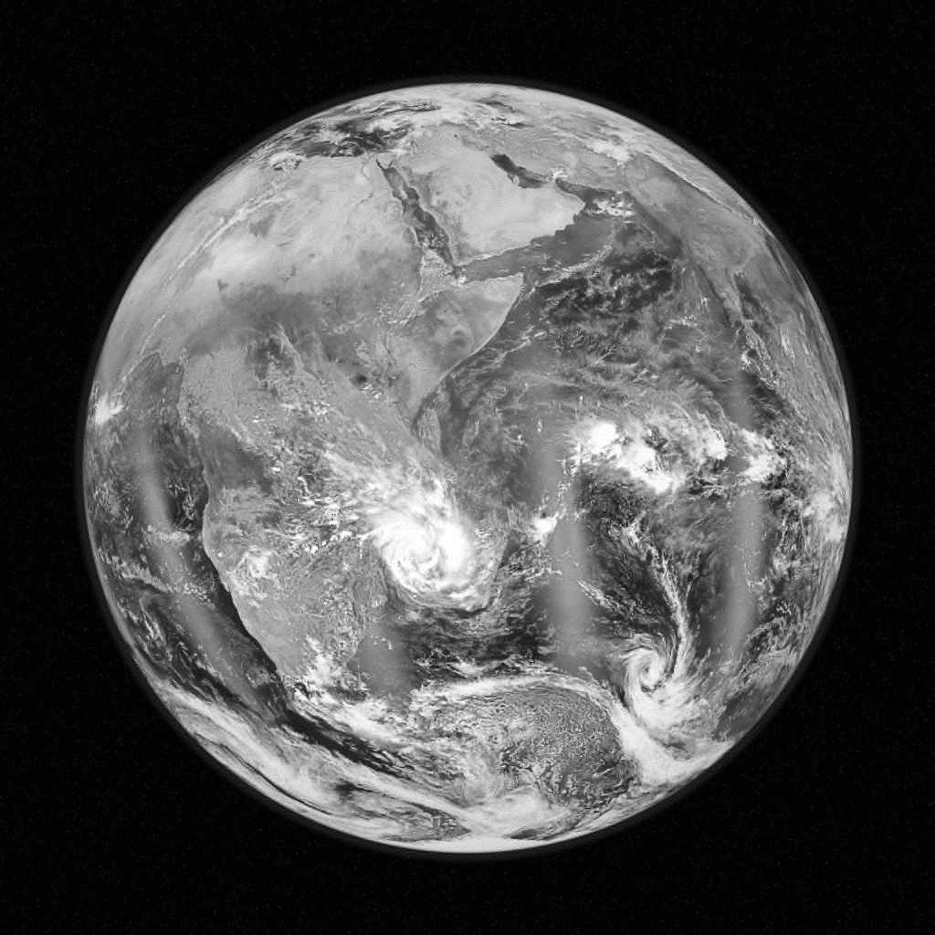
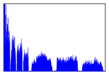
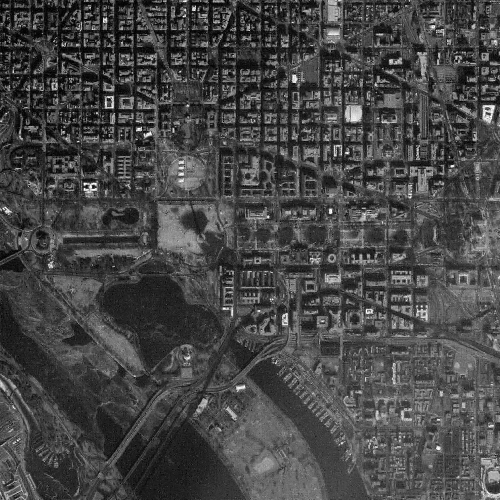
(a) Two image reconstructions from 20% of their Fourier coefficients at $1024\!\times\!1024$ chosen according to a multilevel sampling scheme. The upper-right inset shows the wavelet coefficients of the original images.

         

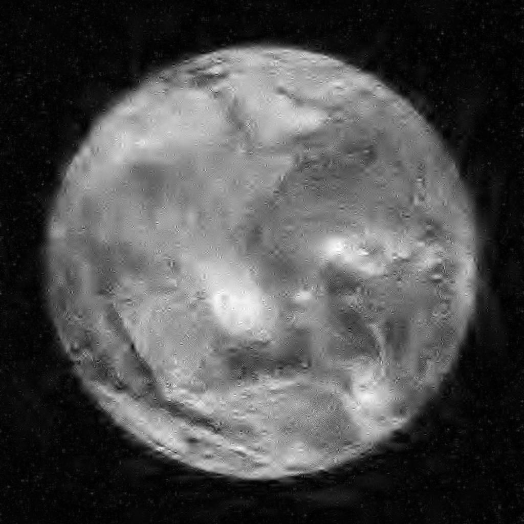
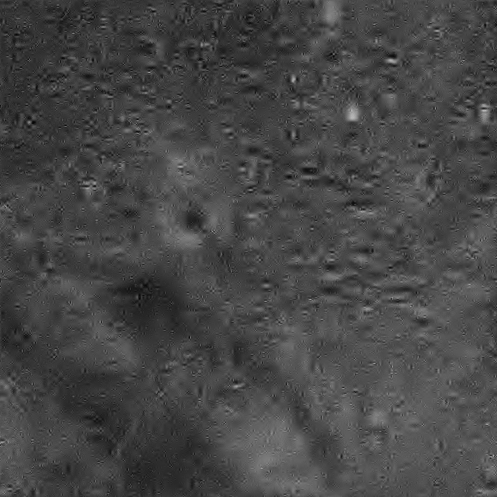
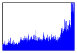
(b) Reversed wavelet coefficients (inset) and the reconstructions from the reversed coefficients at $1024\!\times\!1024$, using the same subsampling patterns used above in (a).

Figure 25: Reconstructions of two images using wavelet coefficients (top) and reversed wavelet coefficients (bottom).

4.10 Third consequence: no Restricted Isometry Propery (RIP)

Let us recall the definition of the restricted isometry property [EldarKutyniokCSBook, FoucartRauhutCSbook]:

Definition 4.13.

A matrix $A$ satisfies the the Restricted Isometry Property (RIP) of order $k$ if there exists a $\delta_{k}$ such that

$$(1-\delta_{k})\|x\|^{2}\leq\|Ax\|^{2}\leq(1+\delta_{k})\|x\|^{2}$$

holds for all $k$-sparse vectors $x$.

A standard theorem in CS is the following:

Theorem 4.14.

Suppose that $A$ satisfies the RIP of order $2k$ with $\delta_{2k}<\sqrt{2}-1$ and we obtain measurements of the form $y=Ax$, then any minimiser $\hat{x}$ of

$$\min\|z\|_{\ell^{1}}\quad\text{subject to}\,\,Az=y$$

satisfies

$$\|\hat{x}-x\|\leq C_{0}\frac{\sigma_{k}(x)_{1}}{\sqrt{k}}.$$ (4.31)

In this case recall that

$$\sigma_{k}(x)_{1}:=\min_{y\in\Sigma_{k}}\|x-y\|_{\ell^{1}},$$

where $\Sigma_{k}$ denotes the set of $k$-sparse vectors. What Theorem 4.14 says is that when $A$ satisfies the RIP, the ordering of the non-zero coefficients does not matter. Thus, there is a very easy numerical experiment that can be carried out in order to determine whether or not the RIP holds in practice: namely, the experiment done in Example 4.9. In particular, the ordering of the coefficients of $x$ is reversed to make $\tilde{x}$, new measurements are created i.e. $\tilde{y}=A\tilde{x}$, a reconstruction $\hat{x}_{1}$ is obtained by $\ell^{1}$-optimization, and finally reversing the ordering of $\hat{x}_{1}$ gives $\hat{x}_{2}$. Note that if the RIP holds then $\hat{x}_{2}$ should also satisfy the error bound (4.31). As demonstrated in Figures 25(a) and 25(b) this is certainly not the case for Fourier and wavelet sensing matrices.

We remark that this is but one example of this phenomenon. Similar tests can be done with essentially any operator that stems from an infinite-dimensional problem where one will observe asymptotic incoherence and asymptotic sparsity. Note that this includes virtually all problems in medical imaging.

The RIP is a popular tool for analyzing CS algorithms. In fact, it is possible to prove that given enough measurements (or equivalently, a sufficiently small sparsity) the RIP will hold for Fourier sampling with Haar wavelets [KrahmerWardCSImaging]. However, the above experiment clearly indicates that for realistic subsampling percentages and realistic sparsities, the observed reconstruction quality is not explained by a RIP. In view of this, the third conclusion of our work is that the RIP is of limited value in analyzing compressive imaging strategies. Simply put, the RIP leads to highly pessimistic estimates on the number of measurements required over that which is actually necessary in practice. (Asymptotic) coherence, on the other hand, is both a relevant and powerful tool for understanding recoverability in this setting.

5 Acknowledgments

The authors would like to thank Milana Gataric and Clarice Poon for providing several MATLAB codes used in this paper. Anders Hansen acknowledges support from a Royal Society University Research Fellowship as well as UK Engineering and Physical Sciences Research Council (EPSRC) grant EP/L003457/1.

References

- [1] \harvarditem[Adcock & Hansen]Adcock & Hansen2011aBAACHGSCS Adcock, B. & Hansen, A. C. (2011a), ‘Generalized sampling and infinite-dimensional compressed sensing’, Technical report NA2011/02, DAMTP, University of Cambridge.
- [2] \harvarditem[Adcock & Hansen]Adcock & Hansen2011bBAACHSampTA Adcock, B. & Hansen, A. C. (2011b), Reduced consistency sampling in Hilbert spaces, in ‘Proceedings of the 9th International Conference on Sampling Theory and Applications’.
- [3] \harvarditem[Adcock & Hansen]Adcock & Hansen2012aBAACHShannon Adcock, B. & Hansen, A. C. (2012a), ‘A generalized sampling theorem for stable reconstructions in arbitrary bases’, J. Fourier Anal. Appl. 18(4), 685–716.
- [4] \harvarditem[Adcock & Hansen]Adcock & Hansen2012bBAACHAccRecov Adcock, B. & Hansen, A. C. (2012b), ‘Stable reconstructions in Hilbert spaces and the resolution of the Gibbs phenomenon’, Appl. Comput. Harmon. Anal. 32(3), 357–388.
- [5] \harvarditem[Adcock & Hansen]Adcock & Hansen2013AdcockHansenSpecData Adcock, B. & Hansen, A. C. (2013), ‘Generalized sampling and the stable and accurate reconstruction of piecewise analytic functions from their Fourier coefficients’, Math. Comp. (to appear).
- [6] \harvarditem[Adcock et al.]Adcock, Hansen & Poon2013aBAACHOptimality Adcock, B., Hansen, A. C. & Poon, C. (2013a), ‘Beyond consistent reconstructions: optimality and sharp bounds for generalized sampling, and application to the uniform resampling problem.’, SIAM J. Math. Anal. (to appear).
- [7] \harvarditem[Adcock et al.]Adcock, Hansen & Poon2013bAHPWavelet Adcock, B., Hansen, A. C. & Poon, C. (2013b), ‘On optimal wavelet reconstructions from Fourier samples: linearity and universality of the stable sampling rate’, Appl. Comput. Harmon. Anal. (to appear).
- [8] \harvarditem[Adcock et al.]Adcock, Hansen & Shadrin2012AdcockHansenShadrinStabilityFourier Adcock, B., Hansen, A. C. & Shadrin, A. (2012), ‘A stability barrier for reconstructions from Fourier samples’, Preprint.
- [9] \harvarditem[Adcock et al.]Adcock, Hansen, Herrholz & Teschke2013cAHHTillposed Adcock, B., Hansen, A. C., Herrholz, E. & Teschke, G. (2013c), ‘Generalized sampling: extension to frames and inverse and ill-posed problems’, Inverse Problems 29(1), 015008.
- [10] \harvarditem[Adcock et al.]Adcock, Hansen, Poon & Roman2013dAHPRBreaking Adcock, B., Hansen, A. C., Poon, C. & Roman, B. (2013d), ‘Breaking the coherence barrier: asymptotic incoherence and asymptotic sparsity in compressed sensing’, Preprint.
- [11] \harvarditem[Adcock et al.]Adcock, Huybrechs & Martín-Vaquero2013eFEStability Adcock, B., Huybrechs, D. & Martín-Vaquero, J. (2013e), ‘On the numerical stability of Fourier extensions’, Found. Comput. Math. (to appear).
- [12] \harvarditem[Beylkin]Beylkin1985beylkin99seismic Beylkin, G. (1985), ‘Imaging of discontinuities in the inverse scattering problem by inversion of a causal generalized radon transform’, J. Math. Phys. 26(1), 99–108.
- [13] \harvarditem[Bleistein et al.]Bleistein, Cohen & Stockwell2001bleistein2001seismic Bleistein, N., Cohen, J. K. & Stockwell, J. J. W. (2001), Mathematics of Multidimensional Seismic Imaging, Migration, and Inversion, Vol. 13, Springer.
- [14] \harvarditem[Borcea]Borcea2002borcea2002eit Borcea, L. (2002), ‘Electrical impedance tomography’, Inverse problems 18(6), R99–R136.
- [15] \harvarditem[Borden & Cheney]Borden & Cheney2005borden2005synthetic Borden, B. & Cheney, M. (2005), ‘Synthetic-aperture imaging from high-Doppler-resolution measurements’, Inverse Problems 21(1), 1.
- [16] \harvarditem[Böttcher]Böttcher1996bottcher1996 Böttcher, A. (1996), Infinite matrices and projection methods, in ‘Lectures on operator theory and its applications (Waterloo, ON, 1994)’, Vol. 3 of Fields Inst. Monogr., Amer. Math. Soc., Providence, RI, pp. 1–72.
- [17] \harvarditem[Buckholtz]Buckholtz1999BuckholtzIdempotents Buckholtz, D. (1999), ‘Hilbert space idempotents and involutions’, Proc. Amer. Math. Soc. 128, 1415–1418.
- [18] \harvarditem[Candès]Candès2008candesCSMag Candès, E. J. (2008), ‘An introduction to compressive sensing’, IEEE Signal Process. Mag. 25(2), 21–30.
- [19] \harvarditem[Candès & Donoho]Candès & Donoho2004candes2004new Candès, E. J. & Donoho, D. (2004), ‘New tight frames of curvelets and optimal representations of objects with piecewise singularities’, Comm. Pure Appl. Math. 57(2), 219–266.
- [20] \harvarditem[Candès & Fernandez-Granda]Candès & Fernandez-Granda2012CandesSuperresolution Candès, E. J. & Fernandez-Granda, C. (2012), ‘Towards a mathematical theory of super-resolution’, Comm. Pure Appl. Math. (to appear).
- [21] \harvarditem[Candès & Plan]Candès & Plan2011Candes_Plan Candès, E. J. & Plan, Y. (2011), ‘A probabilistic and RIPless theory of compressed sensing’, IEEE Trans. Inform. Theory 57(11), 7235–7254.
- [22] \harvarditem[Candès & Romberg]Candès & Romberg2007Candes_Romberg Candès, E. J. & Romberg, J. (2007), ‘Sparsity and incoherence in compressive sampling’, Inverse Problems 23(3), 969–985.
- [23] \harvarditem[Christensen]Christensen2003christensen2003introduction Christensen, O. (2003), An Introduction to Frames and Riesz Bases, Birkhauser.
- [24] \harvarditem[Cohen et al.]Cohen, Daubechies & Vial1993CDVwavelets Cohen, A., Daubechies, I. & Vial, P. (1993), ‘Wavelet bases on the interval and fast algorithms’, Appl. Comput. Harmon. Anal. 1, 54–81.
- [25] \harvarditem[De Hoop et al.]De Hoop, Smith, Uhlmann & Van der Hilst2009dehoop2009seismic De Hoop, M. V., Smith, H., Uhlmann, G. & Van der Hilst, R. D. (2009), ‘Seismic imaging with the generalized Radon transform: A curvelet transform perspective’, Inverse Problems 25(2), 025005.
- [26] \harvarditem[Do & Vetterli]Do & Vetterli2005Vetterli Do, M. N. & Vetterli, M. (2005), ‘The contourlet transform: An efficient directional multiresolution image representation’, IEEE Transactions on Image Processing 14(12), 2091–2106.
- [27] \harvarditem[Donoho]Donoho2006donohoCS Donoho, D. L. (2006), ‘Compressed sensing’, IEEE Trans. Inform. Theory 52(4), 1289–1306.
- [28] \harvarditem[Dvorkind & Eldar]Dvorkind & Eldar2009EldarRobConsistSamp Dvorkind, T. & Eldar, Y. C. (2009), ‘Robust and consistent sampling’, IEEE Signal Process. Letters 16(9), 739–742.
- [29] \harvarditem[Eldar]Eldar2003aeldar2003FAA Eldar, Y. C. (2003a), ‘Sampling with arbitrary sampling and reconstruction spaces and oblique dual frame vectors’, J. Fourier Anal. Appl. 9(1), 77–96.
- [30] \harvarditem[Eldar]Eldar2003beldar2003sampling Eldar, Y. C. (2003b), ‘Sampling without input constraints: Consistent reconstruction in arbitrary spaces’, Sampling, Wavelets and Tomography.
- [31] \harvarditem[Eldar & Dvorkind]Eldar & Dvorkind2006EldarMinimax Eldar, Y. C. & Dvorkind, T. (2006), ‘A minimum squared-error framework for generalized sampling’, IEEE Trans. Signal Process. 54(6), 2155–2167.
- [32] \harvarditem[Eldar & Kutyniok]Eldar & Kutyniok2012EldarKutyniokCSBook Eldar, Y. C. & Kutyniok, G., eds (2012), Compressed Sensing: Theory and Applications, Cambridge University Press.
- [33] \harvarditem[Eldar & Werther]Eldar & Werther2005eldar2005general Eldar, Y. C. & Werther, T. (2005), ‘General framework for consistent sampling in Hilbert spaces’, Int. J. Wavelets Multiresolut. Inf. Process. 3(3), 347.
- [34] \harvarditem[Engl et al.]Engl, Hanke & Neubauer1996EnglRegularization Engl, H. W., Hanke, M. & Neubauer, A. (1996), Regularization of Inverse Problems, Kluwer Academic, Dordrecht, The Netherlands.
- [35] \harvarditem[Foucart & Rauhut]Foucart & Rauhut2013FoucartRauhutCSbook Foucart, S. & Rauhut, H. (2013), A Mathematical Introduction to Compressive Sensing, Birkhauser.
- [36] \harvarditem[Gröchenig et al.]Gröchenig, Rzeszotnik & Strohmer2011strohmer Gröchenig, K., Rzeszotnik, Z. & Strohmer, T. (2011), ‘Quantitative estimates for the finite section method and Banach algebras of matrices’, Integral Equations and Operator Theory 67(2), 183–202.
- [37] \harvarditem[Guerquin-Kern et al.]Guerquin-Kern, Häberlin, Pruessmann & Unser2011PruessmannUnserMRIFast Guerquin-Kern, M., Häberlin, M., Pruessmann, K. P. & Unser, M. (2011), ‘A fast wavelet-based reconstruction method for Magnetic Resonance Imaging’, IEEE Trans. Med. Imaging 30(9), 1649–1660.
- [38] \harvarditem[Guerquin-Kern et al.]Guerquin-Kern, Lejeune, Pruessmann & Unser2012GLPU Guerquin-Kern, M., Lejeune, L., Pruessmann, K. P. & Unser, M. (2012), ‘Realistic analytical phantoms for parallel Magnetic Resonance Imaging’, IEEE Trans. Med. Imaging 31(3), 626–636.
- [39] \harvarditem[Hagen et al.]Hagen, Roch & Silbermann2001hagen2001c Hagen, R., Roch, S. & Silbermann, B. (2001), -Algebras and Numerical Analysis, Vol. 236 of Monographs and Textbooks in Pure and Applied Mathematics, Marcel Dekker Inc., New York.
- [40] \harvarditem[Hansen]Hansen2008hansen2008 Hansen, A. C. (2008), ‘On the approximation of spectra of linear operators on Hilbert spaces’, J. Funct. Anal. 254(8), 2092–2126.
- [41] \harvarditem[Hansen]Hansen2011hansen2011 Hansen, A. C. (2011), ‘On the solvability complexity index, the n-pseudospectrum and approximations of spectra of operators’, J. Amer. Math. Soc. 24(1), 81–124.
- [42] \harvarditem[Hansen]Hansen2010hansen_discrete_2010 Hansen, P. C. (2010), Discrete Inverse Problems: Insight and Algorithms, Fundamentals of algorithms; Variation: Fundamentals of algorithms., Society for Industrial and Applied Mathematics, Philadelphia.
- [43] \harvarditem[Heike]Heike1986heike1986spect Heike, U. (1986), ‘Single-photon emission computed tomography by inverting the attenuated Radon transform with least-squares collocation’, Inverse Problems 2(3), 307–330.
- [44] \harvarditem[Heinemeyer et al.]Heinemeyer, Lindner & Potthast2008Lindner2008 Heinemeyer, E., Lindner, M. & Potthast, R. (2008), ‘Convergence and numerics of a multisection method for scattering by three-dimensional rough surfaces’, SIAM J. Numer. Anal. 46(4), 1780–1798.
- [45] \harvarditem[Hirabayashi & Unser]Hirabayashi & Unser2007UnserHirabayashiConsist Hirabayashi, A. & Unser, M. (2007), ‘Consistent sampling and signal recovery’, IEEE Trans. Signal Process. 55(8), 4104–4115.
- [46] \harvarditem[Jones et al.]Jones, Adcock & Hansen2013Jones2013Incoherence Jones, A. D., Adcock, B. & Hansen, A. C. (2013), ‘On asymptotic incoherence and its implications for compressed sensing for inverse problems’, In preparation.
- [47] \harvarditem[Kaipio & Somersalo]Kaipio & Somersalo2007Kaipio Kaipio, J. & Somersalo, E. (2007), ‘Statistical inverse problems: discretization, model reduction and inverse crimes’, J. Comput. Appl. Math. 198(2), 493–504.
- [48] \harvarditem[Krahmer & Ward]Krahmer & Ward2012KrahmerWardCSImaging Krahmer, F. & Ward, R. (2012), ‘Compressive imaging: stable and robust recovery from variable density frequency samples’, Preprint.
- [49] \harvarditem[Kuchment]Kuchment2006kuchment2006genradon Kuchment, P. (2006), Generalized transforms of Radon type and their applications, in ‘The Radon transform, inverse problems, and tomography’, Vol. 63, American Mathematical Society, pp. 67–91.
- [50] \harvarditem[Kuchment & Kunyansky]Kuchment & Kunyansky2011kuchment2011pattat Kuchment, P. & Kunyansky, L. (2011), Mathematics of photoacoustic and thermoacoustic tomography, in O. Scherzer, ed., ‘Handbook of Mathematical Methods in Imaging’, Springer New York, pp. 817–865.
- [51] \harvarditem[Kutyniok et al.]Kutyniok, Lemvig & Lim2012Gitta3 Kutyniok, G., Lemvig, J. & Lim, W.-Q. (2012), Compactly supported shearlets, in M. Neamtu & L. Schumaker, eds, ‘Approximation Theory XIII: San Antonio 2010’, Vol. 13 of Springer Proceedings in Mathematics, Springer New York, pp. 163–186.
- [52] \harvarditem[Lawrence et al.]Lawrence, Phan & Ellisman2012lawrence2012et Lawrence, A. F., Phan, S. & Ellisman, M. (2012), Electron tomography and multiscale biology, in M. Agrawal, S. Cooper & A. Li, eds, ‘Theory and Applications of Models of Computation’, Vol. 7287 of Lecture Notes in Computer Science, Springer Berlin Heidelberg, pp. 109–130.
- [53] \harvarditem[Leary et al.]Leary, Saghi, Midgley & Holland2013leary2013etcs Leary, R., Saghi, Z., Midgley, P. A. & Holland, D. J. (2013), ‘Compressed sensing electron tomography’, Ultramicroscopy 131(0), 70–91.
- [54] \harvarditem[Lindner]Lindner2006lindner2006 Lindner, M. (2006), Infinite Matrices and their Finite Sections, Frontiers in Mathematics, Birkhäuser Verlag, Basel. An introduction to the limit operator method.
- [55] \harvarditem[Liu et al.]Liu, Liu, Wang & Yang2010liu2010barcode Liu, F., Liu, A., Wang, M. & Yang, Z. (2010), Robust and fast localization algorithm for data matrix barcode, in ‘Optoelectronics and Image Processing (ICOIP), 2010 International Conference on’, Vol. 2, IEEE, pp. 356–359.
- [56] \harvarditem[Louis]Louis1989LouisInverse Louis, A. K. (1989), Inverse und schlecht gestellte Probleme, Teubner, Stuttgart.
- [57] \harvarditem[Lustig et al.]Lustig, Donoho, Santos & Pauly2008Lustig Lustig, M., Donoho, D. L., Santos, J. M. & Pauly, J. M. (2008), ‘Compressed Sensing MRI’, IEEE Signal Process. Mag. 25(2), 72–82.
- [58] \harvarditem[Mallat]Mallat2009mallat09wavelet Mallat, S. G. (2009), A Wavelet Tour of Signal Processing: The Sparse Way, 3 edn, Academic Press.
- [59] \harvarditem[Mueller & Siltanen]Mueller & Siltanen2012Mller Mueller, J. L. & Siltanen, S. (2012), Linear and Nonlinear Inverse Problems with Practical Applications, Society for Industrial and Applied Mathematics, Philadelphia, PA, USA.
- [60] \harvarditem[Natterer & Wubbeling]Natterer & Wubbeling2001natterer2001imagerec Natterer, F. & Wubbeling, F. (2001), Mathematical methods in image reconstruction, Society for Industrial and Applied Mathematics, Philadelphia, PA, USA.
- [61] \harvarditem[Poon]Poon2013GSl1 Poon, C. (2013), ‘A stable and consistent approach to generalized sampling’, Preprint.
- [62] \harvarditem[Quinto]Quinto2006quinto2006xrayradon Quinto, E. T. (2006), An introduction to X-ray tomography and Radon transforms, in ‘The Radon transform, inverse problems, and tomography’, Vol. 63, American Mathematical Society, pp. 1–23.
- [63] \harvarditem[Roulston & Muhleman]Roulston & Muhleman1997roulston1997polar Roulston, M. S. & Muhleman, D. O. (1997), ‘Synthesizing radar maps of polar regions with a Doppler-only method’, Applied optics 36(17), 3912–3919.
- [64] \harvarditem[Shepp & Srivastava]Shepp & Srivastava1978shepp1978ct Shepp, L. A. & Srivastava, S. (1978), ‘Computerized Tomography: The new medical X-ray technology’, Amer. Math. Monthly 45, 429–439.
- [65] \harvarditem[Steinberg]Steinberg2000steinberg2000oblique Steinberg, J. (2000), ‘Oblique projections in Hilbert spaces’, Integr. Equ. Oper. Theory 38(1), 81–119.
- [66] \harvarditem[Strang & Nguyen]Strang & Nguyen1996StrangNguyen Strang, G. & Nguyen, T. (1996), Wavelets and Filter Banks, Wellesley-Cambridge Press, Wellesley, MA.
- [67] \harvarditem[Szyld]Szyld2006SzyldOblProj Szyld, D. (2006), ‘The many proofs of an identity on the norm of oblique projections’, Numer. Algorithms 42, 309–323.
- [68] \harvarditem[Tang]Tang1999Tang1999Oblique Tang, W.-S. (1999), ‘Oblique projections, biorthogonal Riesz bases and multiwavelets in Hilbert spaces’, Proc. Amer. Math. Soc. 128(2), 463–473.
- [69] \harvarditem[Trefethan & Bau III]Trefethan & Bau III1997TrefethenBau Trefethan, L. N. & Bau III, D. (1997), Numerical Linear Algebra, SIAM, Philadephia.
- [70] \harvarditem[Trefethen]Trefethen2013TrefethenATAP Trefethen, L. N. (2013), Approximation Theory and Aproximation Practice, SIAM.
- [71] \harvarditem[Unser]Unser2000unser2000sampling Unser, M. (2000), ‘Sampling–50 years after Shannon’, Proc. IEEE 88(4), 569–587.
- [72] \harvarditem[Unser & Aldroubi]Unser & Aldroubi1994unser1994general Unser, M. & Aldroubi, A. (1994), ‘A general sampling theory for nonideal acquisition devices’, IEEE Trans. Signal Process. 42(11), 2915–2925.
- [73] \harvarditem[Unser & Zerubia]Unser & Zerubia1998unserzerubia Unser, M. & Zerubia, J. (1998), ‘A generalized sampling theory without band-limiting constraints’, IEEE Trans. Circuits Syst. II. 45(8), 959–969.
- [74]