Boolean decision problems with competing interactions on scale-free networks:
Equilibrium and nonequilibrium behavior in an external bias

Abstract

We study the equilibrium and nonequilibrium properties of Boolean decision problems with competing interactions on scale-free networks in an external bias (magnetic field). Previous studies at zero field have shown a remarkable equilibrium stability of Boolean variables (Ising spins) with competing interactions (spin glasses) on scale-free networks. When the exponent that describes the power-law decay of the connectivity of the network is strictly larger than 3, the system undergoes a spin-glass transition. However, when the exponent is equal to or less than 3, the glass phase is stable for all temperatures. First, we perform finite-temperature Monte Carlo simulations in a field to test the robustness of the spin-glass phase and show that the system has a spin-glass phase in a field, i.e., exhibits a de Almeida–Thouless line. Furthermore, we study avalanche distributions when the system is driven by a field at zero temperature to test if the system displays self-organized criticality. Numerical results suggest that avalanches (damage) can spread across the whole system with nonzero probability when the decay exponent of the interaction degree is less than or equal to 2, i.e., that Boolean decision problems on scale-free networks with competing interactions can be fragile when not in thermal equilibrium.

I Introduction

Scale-free networks play an integral role in nature, as well as industrial, technological and sociological applications Albert et al. (1999). In these networks, the edge degrees $\{k_{i}\}$ (the number of neighbors each node has) are distributed according to a power law $\lambda$, with the probability $\wp_{k}$ for a node to have $k$ neighbors given by

$$\wp_{k} \propto k^{-\lambda}.$$ (1)

In the meantime, there have been many studies of Boolean variables on scale-free networks Bartolozzi et al. (2006); Herrero (2009); Lee et al. (2006); Weigel and Johnston (2007) and, more recently, even with competing interactions Mooij and Kappen (2004); Kim et al. (2005); Ferreira et al. (2010); Ostilli et al. (2011); Katzgraber et al. (2012). There is general consensus that stable ferromagnetic and spin-glass phases emerge in these complex systems Katzgraber et al. (2012) and that for particular choices of the decay exponent $\lambda$ the critical temperature diverges, i.e., Boolean variables with competing interactions are extremely robust to local perturbations.

However, the behavior of these intriguing systems in an external magnetic field—which can be interpreted as a global bias—remains to be fully understood. Although a replica ansatz works well when determining the critical temperature of the system Kim et al. (2005); Katzgraber et al. (2012) in zero field, it is unclear if a stable spin-glass state persists in a field. In addition, when studying the system without local perturbations (i.e., at zero temperature), it is unclear if “damage” in the form of avalanches of Boolean variable flips triggered by a field can spread easily across the system.

In this work we tackle the two aforementioned problems numerically and show that at finite temperature Boolean variables with competing interactions are remarkably robust to global external biases. In particular, we show that a de Almeida–Thouless line de Almeida and Thouless (1978) persists to a regime of $\lambda$ where the system is not in the mean-field Sherrington-Kirkpatrick Sherrington and Kirkpatrick (1975) universality class, i.e., when $\lambda<4$ Kim et al. (2005); Katzgraber et al. (2012).

Furthermore, we probe for the existence of self-organized criticality (SOC) when driving the system at zero temperature with an external magnetic field across a hysteresis loop. SOC is a property of large dissipative systems to drive themselves into a scale-invariant critical state without any special parameter tuning Newman and Stein (1994); Cieplak et al. (1994); Schenk et al. (2002); Pázmándi et al. (1999); Gonçalves and Boettcher (2008). It is a phenomenon found in many problems ranging from earthquake statistics to the structure of galaxy clusters. As such, studying SOC on scale-free networks might help us gain a deeper understanding on how avalanches, i.e., large-scale perturbations, might spread across scale-free networks that are so omnipresent in nature. Recent simulations Andresen et al. (2013) have shown that a diverging number of neighbors is the key ingredient to obtain SOC in glassy spin systems. In scale-free graphs the average edge degree diverges if $\lambda\leq 2$. As such, it might be conceivable that in this regime spin glasses on scale-free graphs exhibit SOC. However, it is unclear what happens for $\lambda>2$ where the number of neighbors each spin has is finite in the thermodynamic limit, or how the fraction of ferromagnetic versus antiferromagnetic bonds influences the scaling of the avalanche distributions. Within the spin-glass phase, for Gaussian disorder and bimodal disorder with the same fraction $p$ of ferromagnetic and antiferromagnetic bonds, we find that when $\lambda\leq 2$ Boolean variables with competing interactions always display SOC like the mean-field Sherrington-Kirkpatrick model Pázmándi et al. (1999). For $\lambda>2$ and with bimodal disorder, a critical line in the $p$–$\lambda$ plane emerges along which perturbations to the system are scale free, but not self-organized critical because the fraction of ferromagnetic bonds has to be carefully tuned. The latter is reminiscent of the behavior found in the random-field Ising model Sethna et al. (1993); Perkovic et al. (1995, 1999); Kuntz et al. (1998); Sethna et al. (2004), as well as random-bond Vives and Planes (1994) and random-anisotropy Ising models Vives and Planes (2001).

The paper is structured as follows. Section II introduces the Hamiltonian studied, followed by numerical details, observables, and results from equilibrium Monte Carlo simulations in Sec. III. Section IV presents our results on nonequilibrium avalanches on scale-free graphs, followed by concluding remarks. In the appendix we outline our analytical calculations to determine the de Almeida–Thouless for spin glasses on scale-free graphs.

II Model

The Hamiltonian of the Edwards-Anderson Ising spin glass on a scale-free graph in an external magnetic field is given by

$${\mathcal{H}}(\{s_{i}\})=-\sum_{i<j}^{N}J_{ij}\varepsilon_{ij}s_{i}\,s_{j}-\sum_{i}H_{i}s_{i},$$ (2)

where the Ising spins $s_{i}\in\{\pm 1\}$ lie on the vertices of a scale-free graph with $N$ sites and the interactions are given by

$${\mathcal{P}}(J_{ij},\varepsilon_{ij})=\wp_{J}(J_{ij})\left[\Big{(}1-\frac{K}{N}\Big{)}\delta(\varepsilon_{ij})+\frac{K}{N}\delta(\varepsilon_{ij}-1)\right].$$ (3)

If a bond is present, we set $\varepsilon_{ij}=1$, otherwise $\varepsilon_{ij}=0$. $K$ represents the mean connectivity of the scale-free graph. The connectivity of site $i$, $k_{i}:=\sum_{j}\varepsilon_{ij}$, is sampled from a scale-free distribution as done in Ref. Katzgraber et al. (2012). The interactions between the spins $J_{ij}$ are independent random variables drawn from a Gaussian distribution with zero mean and standard deviation unity, i.e.,

$$\wp_{J}(J_{ij})\sim\exp{(-J_{ij}^{2}/2)}\,.$$ (4)

In the nonequilibrium studies we also study bimodal-distributed disorder where we can change the fraction of ferromagnetic bonds $p$, i.e.,

$$\wp_{J}(J_{ij})=p\delta(J_{ij}+1)+(1-p)\delta(J_{ij}-1)\,.$$ (5)

Finally, for the finite-temperature studies we use random fields drawn from a Gaussian distribution with zero mean and standard deviation $H_{r}$ in Eq. (2), instead of a uniform field. This allows us to perform a detailed equilibration test of the Monte Carlo method Katzgraber et al. (2001, 2009).

The scale-free graphs are generated using preferential attachment with slight modifications Barabasi and Albert (1999). Details of the method are described in Ref. Katzgraber et al. (2012). We impose an upper bound on the allowed edge degrees, $k_{\mathrm{max}}=\sqrt{N}$. Although we can, in principle, generate graphs with $k$ exceeding $\sqrt{N}$, the ensemble is poorly defined in this case: Even randomly chosen graphs cannot be uncorrelated Burda and Krzywicki (2003); Boguñá et al. (2004); Catanzaro et al. (2005). Furthermore, to prevent dangling ends that do not contribute to frustrated loops in the system, we set a lower bound to the edge degree, namely $k_{\mathrm{min}}=3$.

III Equilibrium properties in a field

In equilibrium, the behavior of spin glasses in a magnetic field is controversial Young and Katzgraber (2004); Katzgraber and Young (2005); Jörg et al. (2008); Katzgraber et al. (2009); Baños et al. (2012); Baity-Jesi et al. (2013). While the infinite-range (mean-field) Sherrington-Kirkpatrick (SK) model Sherrington and Kirkpatrick (1975) has a line of transitions at finite field known as the de Almeida–Thouless (AT) line de Almeida and Thouless (1978) that separates the spin-glass phase from the paramagnetic phase at finite fields or temperatures, it has not been definitely established whether an AT line occurs in systems with short-range interactions. Spin glasses on scale-free networks are somewhat “in between” the infinite-range and short-range limits depending on the exponent $\lambda$. As such, it is unclear if a spin-glass state will persist when an external field $H$ is applied, especially when the spin-glass transition at zero field occurs at finite temperatures, i.e., for $\lambda>3$.

Note that spin glasses on scale-free graphs share the same universality class as the SK model if $\lambda>4$ Katzgraber et al. (2012). As such, in this regime, one can expect an AT line. However, for $3<\lambda<4$, where $T_{c}<\infty$, the critical exponents depend on the exponent $\lambda$ Kim et al. (2005); Katzgraber et al. (2012). Therefore, it is unclear if a spin-glass state in a field will persist. For $\lambda\leq 3$ the critical temperature diverges with the system size, i.e., we also expect the system to have a spin-glass state for finite fields. We therefore focus on two values of $\lambda$, namely $\lambda=4.50$ (deep within the SK-like regime because $\lambda=4$ has logarithmic corrections) Katzgraber et al. (2012) and $\lambda=3.75$ (where the existence of an AT line remains to be determined).

III.1 Observables

In simulations, it is most desirable to perform a finite-size scaling (FSS) of dimensionless quantities. One such quantity, the Binder ratio Binder (1981), turns out to be poorly behaved in an external field in short-range systems Ciria et al. (1993). Therefore, to determine the location of a spin-glass phase transition we measure the connected spin-glass susceptibility given by

$$\chi=\frac{1}{N}\displaystyle\sum_{i,j}[\left(\langle{s_{i}s_{j}}\rangle_{T}-\langle{s_{i}}\rangle_{T}\langle{s_{j}}\rangle_{T}\right)^{2}]_{\rm av},$$ (6)

where $\langle\cdots\rangle_{T}$ denotes a thermal average and $[\cdots]_{\rm av}$ an average over both the bond disorder and different network instances. $N$ is the number of spins. To avoid bias, each thermal average is obtained from separate copies (replicas) of the spins. This means that we simulate four independent replicas at each temperature.

For any spin glass outside the mean-field regime, the scaling behavior of the susceptibility is given by Katzgraber et al. (2012)

$$\chi=N^{2-\eta}\widetilde{C}\left(N^{1/\nu}[\beta-\beta_{c}]\right)\,,$$ (7)

where $\nu$ and $\eta$ are the correlation length and susceptibility exponents, respectively, and $\beta_{c}=1/T_{c}$ is the inverse temperature for a given field strength $H_{r}$.

For $\lambda<4$ (see the appendix for details) we expect the critical exponent $\gamma=1$. This is only possible if $2-\eta=1/\nu$ in Eq. (7). Using the standard scaling relation $\alpha+2\beta+\gamma=2$, the hyperscaling relation $d\nu=2-\alpha$ (which we assume will hold when $\lambda<4$), and allowing for the nonstandard meaning of $\nu$ in this paper (it is equal to $d\nu$ in standard notation where $d$ is here the dimensionality of the system), it follows for $\lambda<4$, where $\beta=1/(\lambda-3)$ (see the appendix and Ref. Kim et al. (2005)) that

$$\nu=\frac{\lambda-1}{\lambda-3}\;\;\;\;{\rm and}\;\;\;\;\eta=2-\frac{1}{\nu}.$$ (8)

For the case of $\lambda=3.75$ this means that $\nu=11/3$ and therefore $\eta=2-1/\nu=19/11$. As such, curves of $\chi/N^{3/11}$ should have the same scaling behavior as the Binder ratio.

For $\lambda>4$, the finite-size scaling form presented in Eq. (7) is replaced by Katzgraber et al. (2009); Larson et al. (2013)

$$\chi=N^{1/3}\widetilde{C}\left(N^{1/3}[\beta-\beta_{c}]\right)\,.$$ (9)

In this case the scaling is simpler because the exponents are fixed and independent of $\lambda$, i.e., $1/\nu=2-\eta=1/3$. Here, curves of $\chi/N^{1/3}$ should have the same scaling behavior as the Binder ratio. Performing a finite-size scaling of the data therefore allows one to detect the transition to high precision.

Finally, note that the aforementioned study is, strictly speaking, only valid at zero field. Although $\gamma=1$ across the AT line, there is no explicit calculation of the critical exponent $\beta$ in a field. While our data suggest that the values of the zero-field exponents might be the same as those for finite external fields, the accuracy of our results for the exponents in a field is limited by large finite-size corrections.

III.2 Equilibration scheme and simulation parameters

The simulations are done using the parallel tempering Monte Carlo method Geyer (1991); Hukushima and Nemoto (1996). The spins couple to site-dependent random fields $H_{i}$ chosen from a Gaussian distribution with zero mean $[H_{i}]_{\rm av}=0$ and standard deviation $[H_{i}^{2}]_{\rm av}^{1/2}=H_{r}$. Simulations are performed at zero field as well as at $H_{r}=0.1$, $0.2$, $0.3$, and $0.4$. Using Gaussian disorder, we can use a strong equilibration test to ensure that the data are in thermal equilibrium Katzgraber et al. (2001, 2009, 2012). Here, the internal energy per spin

$$U=(1/N)[\langle{\mathcal{H}}\rangle_{T}]_{\rm av}\,,$$ (10)

with ${\mathcal{H}}$ defined in Eq. (2), has to equate an expression derived from both the link overlap $q_{4}$ given by

$$q_{4}=\frac{1}{N_{b}}\sum_{i,j}\varepsilon_{ij}s_{i}^{\alpha}s_{j}^{\alpha}s_{i}^{\beta}s_{j}^{\beta}\,,$$ (11)

and the spin overlap

$$q=\frac{1}{N_{b}}\sum_{i}s_{i}^{\alpha}s_{i}^{\beta}\,.$$ (12)

Here $\alpha$ and $\beta$ represent two copies of the system with the same disorder and $N_{b}$ represents the number of neighbors each spin has for a given sample (graph instance). Note that because in Eq. (6) we already simulate four replicas, we actually perform an average over all four-replica permutations.

The system is in thermal equilibrium if

$$U=U(q_{4})=-\frac{1}{T}\,\left[\left\langle\frac{N_{b}}{N}\,(1-q_{4})+H_{r}^{2}\,(1-q)\right\rangle\right]_{\rm av}\,.$$ (13)

Sample data are shown in Fig. 1. The energy $U$ computed directly is compared to the energy computed from the link overlap $U(q_{4})$. The data for both quantities approach a limiting value from opposite directions. Once $U=U(q_{4})$, the data for $q^{2}$ (shifted for better viewing in Fig. 1) are also in thermal equilibrium. The simulation parameters are shown in Table 1.

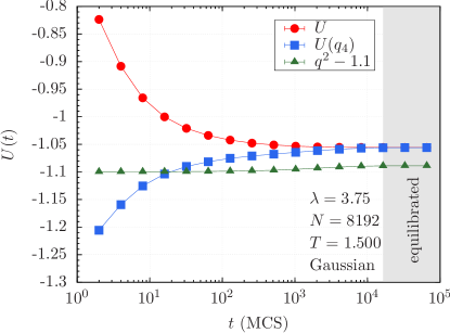
Figure 1: (Color online) Equilibration test for $N=8192$ spins at $T=1.500$ (lowest temperature simulated) and $\lambda=3.75$. Once the data for the energy $U$ and the energy computed from $q_{4}$ [$U(q_{4})$] agree, the system is in thermal equilibrium (shaded area). At this point data for $q^{2}$ are also independent of Monte Carlo time. Note that the data for $q^{2}$ are shifted by a constant factor of $1.1$ for better comparison. Error bars are smaller than the symbols.

Table 1: Parameters of the simulation: For each exponent $\lambda$ and system size $N$, we compute $N_{\rm sa}$ disorder or network instances. $N_{\rm sw}=2^{b}$ is the total number of Monte Carlo sweeps for each of the $4N_{T}$ replicas for a single instance, $T_{\rm min}$ [$T_{\rm max}$] is the lowest [highest] temperature simulated, and $N_{T}$ is the number of temperatures used in the parallel tempering method for each system size $N$.

$\lambda$	$H_{r}$	$N$	$N_{\rm sa}$	$b$	$T_{\rm min}$	$T_{\rm max}$	$N_{T}$
$3.75$	$0.0$	$2048$	$9600$	$16$	$1.5000$	$3.0000$	$30$
$3.75$	$0.0$	$3072$	$9600$	$16$	$1.5000$	$3.0000$	$30$
$3.75$	$0.0$	$4096$	$9600$	$16$	$1.5000$	$3.0000$	$30$
$3.75$	$0.0$	$6144$	$9600$	$16$	$1.5000$	$3.0000$	$30$
$3.75$	$0.0$	$8192$	$9600$	$16$	$1.5000$	$3.0000$	$30$
$3.75$	$0.1$	$512$	$9600$	$17$	$0.9000$	$3.0000$	$50$
$3.75$	$0.1$	$768$	$9600$	$17$	$0.9000$	$3.0000$	$50$
$3.75$	$0.1$	$1024$	$9600$	$17$	$0.9000$	$3.0000$	$50$
$3.75$	$0.1$	$1536$	$9600$	$18$	$0.9000$	$3.0000$	$50$
$3.75$	$0.1$	$2048$	$2400$	$18$	$0.9000$	$3.0000$	$50$
$3.75$	$0.2$	$768$	$9600$	$17$	$0.9000$	$3.0000$	$50$
$3.75$	$0.2$	$1024$	$9600$	$17$	$0.9000$	$3.0000$	$50$
$3.75$	$0.2$	$1536$	$9600$	$18$	$0.9000$	$3.0000$	$50$
$3.75$	$0.2$	$2048$	$2400$	$18$	$0.9000$	$3.0000$	$50$
$3.75$	$0.2$	$4096$	$2400$	$19$	$0.9000$	$3.0000$	$50$
$3.75$	$0.3$	$256$	$9600$	$17$	$0.9000$	$3.0000$	$50$
$3.75$	$0.3$	$512$	$9600$	$18$	$0.9000$	$3.0000$	$50$
$3.75$	$0.3$	$1024$	$9600$	$18$	$0.9000$	$3.0000$	$50$
$3.75$	$0.3$	$2048$	$2400$	$18$	$0.9000$	$3.0000$	$50$
$3.75$	$0.4$	$256$	$9600$	$18$	$0.9000$	$3.0000$	$50$
$3.75$	$0.4$	$512$	$9600$	$18$	$0.9000$	$3.0000$	$50$
$3.75$	$0.4$	$1024$	$9600$	$18$	$0.9000$	$3.0000$	$50$
$3.75$	$0.4$	$2048$	$2400$	$18$	$0.9000$	$3.0000$	$50$
$4.50$	$0.0$	$1024$	$9600$	$16$	$1.0000$	$3.0000$	$30$
$4.50$	$0.0$	$2048$	$9600$	$16$	$1.0000$	$3.0000$	$30$
$4.50$	$0.0$	$4096$	$9600$	$16$	$1.0000$	$3.0000$	$30$
$4.50$	$0.0$	$8192$	$9600$	$16$	$1.0000$	$3.0000$	$30$
$4.50$	$0.1$	$512$	$9600$	$17$	$0.9000$	$3.0000$	$50$
$4.50$	$0.1$	$1024$	$9600$	$17$	$0.9000$	$3.0000$	$50$
$4.50$	$0.1$	$2048$	$9600$	$18$	$0.9000$	$3.0000$	$50$
$4.50$	$0.1$	$4096$	$2400$	$18$	$0.9000$	$3.0000$	$50$
$4.50$	$0.2$	$256$	$9600$	$18$	$0.6000$	$3.0000$	$50$
$4.50$	$0.2$	$512$	$9600$	$18$	$0.6000$	$3.0000$	$50$
$4.50$	$0.2$	$1024$	$9600$	$18$	$0.6000$	$3.0000$	$50$
$4.50$	$0.2$	$2048$	$2400$	$19$	$0.6000$	$3.0000$	$50$
$4.50$	$0.3$	$64$	$9600$	$18$	$0.3000$	$3.0000$	$50$
$4.50$	$0.3$	$128$	$9600$	$19$	$0.3000$	$3.0000$	$50$
$4.50$	$0.3$	$256$	$9600$	$20$	$0.3000$	$3.0000$	$50$
$4.50$	$0.3$	$512$	$9600$	$22$	$0.3000$	$3.0000$	$50$
$4.50$	$0.4$	$90$	$9600$	$19$	$0.3000$	$3.0000$	$50$
$4.50$	$0.4$	$128$	$9600$	$19$	$0.3000$	$3.0000$	$50$
$4.50$	$0.4$	$180$	$9600$	$19$	$0.3000$	$3.0000$	$50$
$4.50$	$0.4$	$256$	$9600$	$20$	$0.3000$	$3.0000$	$50$

III.3 Numerical results for $\lambda=4.50$

Corrections to scaling are large for this model despite the large system sizes and number of samples studied. As previously stated, we expect that for $\lambda=4.50$ a spin-glass state is stable towards an external field because for $\lambda>4$ the system shares the same universality class as the SK model. To determine the AT line, we plot $\chi/N^{1/3}$ versus the inverse temperature $\beta=1/T$. Because $\chi/N^{1/3}$ is a dimensionless function [see Eq. (9)], data for different system sizes should cross at the putative field-dependent transition temperature. To cope with corrections to scaling and obtain a precise estimate of the critical temperature, we study the crossing temperatures $T_{c}(N,2N)$ for pairs of system sizes $N$ and $2N$ assuming

$$T_{c}(N,2N)=T_{c}+A/N^{\omega}\,,$$ (14)

where $A$ is a fitting parameter and empirically $\omega=1$. An example extrapolation is shown in Fig. 2 for $\lambda=4.50$ and $H_{r}=0.1$. A linear fit is very stable and the extrapolation to the thermodynamic limit clear. Statistical error bars are determined via a bootstrap analysis Katzgraber et al. (2006) using the following procedure: For each system size $N$ and $N_{\rm sa}$ disorder realizations, a randomly selected bootstrap sample of $N_{\rm sa}$ disorder realizations is generated. With this random sample, an estimate of $\chi/{N^{1/3}}$ is computed for each temperature. The crossing temperature for pairs of $N$ and $2N$ is obtained by fitting the data to a third-order polynomial and a subsequent root determination. We repeat this procedure $N_{\rm boot}=500$ times for each lattice size and then assemble $N_{\rm boot}$ complete data sets (each having results for every system size $N$) by combining the $i$th bootstrap sample for each size for $i=1$, $\ldots$, $N_{\rm boot}$. The nonlinear fit to Eq. (14) is then carried out on each of these $N_{\rm boot}$ sets, thus obtaining $N_{\rm boot}$ estimates of the fit parameters $T_{c}$ and $A$. Because the bootstrap sampling is done with respect to the disorder realizations which are statistically independent, we can use a conventional bootstrap analysis to estimate statistical error bars on the fit parameters. These are comparable to the standard deviation among the $N_{\rm boot}$ bootstrap estimates.

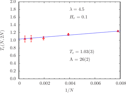
Figure 2: (Color online) Extrapolation to the thermodynamic limit for the critical temperature $T_{c}$ for $\lambda=4.50$ and $H_{r}=0.1$. We determine the crossing points of critical temperatures of the susceptibility expression for pairs of system sizes $N$ and $2N$. Using Eq. (14) with $\omega=1$ we extrapolate the data to the thermodynamic limit. This allows us to take into account corrections to scaling in an unbiased way.

The obtained estimates of $T_{c}$ are listed in Table 2. Figure 3 shows the field–temperature phase diagram for $\lambda=4.50$. The shaded area is intended as a guide to the eye. The critical line separates a paramagnetic (PM) from a spin-glass (SG) phase. The dotted (blue) line represents the AT line computed analytically (appendix) in the limit of $H_{r}\to 0$. For $4<\lambda<5$ the shape of the AT line is given by Eq. (32). The analytical approximation fits the data for $\lambda=4.5$ very well with $H_{r}(T)\sim C_{4.5}(1-T/T_{c})^{5/4}$ and $C_{4.5}=0.48(3)$.

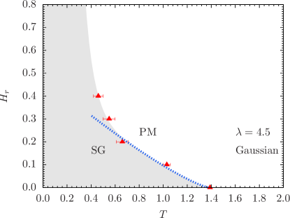
Figure 3: (Color online) Field $H_{r}$ versus temperature $T$ phase diagram for an Ising spin glass on a scale-free graph with $\lambda=4.50$. The data points separate a paramagnetic (PM) from a spin-glass (SG) state. The shaded area is intended as a guide to the eye. The dotted (blue) line is a calculation of the AT line in the $H_{r}\to 0$ limit.

III.4 Numerical results for $\lambda=3.75$

Because for $\lambda<4$ we are no longer in the SK universality class, it is a priori unclear if a spin-glass state in a field will exist. Furthermore, when $\lambda=3.75$, a finite-size scaling according to Eq. (7) has to be performed. Because it is not possible to define a distance metric on a scale-free network, there is no notion of a correlation length or spin-spin correlation function. As such, the critical exponents $\nu$ (that describes the divergence of the correlation length) and $\eta$ (also known as the anomalous dimension) have to be treated carefully. However, we will assume that Eq. (7) is valid in this regime on generic finite-size scaling grounds and treat $\nu$ and $\eta$ as parameters when $H_{r}>0$ with no special meaning attached to them. In addition, we fix $\nu=11/3$ and $\eta=2-1/\nu$ — the zero-field values of the critical exponents — and scale the data at finite fields assuming these exponents are valid also when $H_{r}>0$.

To determine $T_{c}(H_{r})$, we perform a finite-size scaling analysis of the susceptibility data according to Eq. (7). To determine the optimal value of $T_{c}=1/\beta_{c}$ that scales the data best we use the approach developed in Ref. Katzgraber et al. (2006). We assume that the scaling function in Eq. (7) can be represented by a third-order polynomial $y(x)=c_{0}+c_{1}x+c_{2}x^{2}+c_{3}x^{3}$ for $|x|\lesssim 1$ and do a global fit to the seven parameters $c_{i}$ with $i\in\{0,\ldots,3\}$, $\beta_{c}$, $\eta$, and $\nu$. Here $y=\chi/{N^{2-\eta}}$ and $x=N^{1/\nu}[\beta-\beta_{c}]$. After performing a Levenberg-Marquardt minimization combined with a bootstrap analysis we determine the optimal critical parameters with an unbiased statistical error bar.

Figure 4 shows two representative scaling collapses at zero and nonzero field values. The data scale well and allow one to determine the critical temperature with good precision despite the difficulties that scaling the spin-glass susceptibility poses Katzgraber et al. (2006). Note that for zero field we obtain $\eta=1.72(1)$ and $\nu=3.56(17)$, which agree very well with the analytical expressions $\eta=19/11=1.72\ldots$ and $\nu=11/3=3.66\ldots$. However, for finite fields deviations are visible. A summary of the relevant fitting parameters is listed in Table 2. Note that the value of $\eta$ for different fields agrees within error bars. However, fluctuations are larger for $\nu$. One can expect that the universality class of the system does not change along the AT line Binder and Young (1986). Therefore, and because it is hard to simulate large systems for large fields, we also determine $T_{c}$ by fixing $\eta=19/11$ and $\nu=11/3$. As listed in Table 2, both estimates agree within error bars. This is also visible in Fig. 5 which shows the AT line for $\lambda=3.75$. Overall, the analysis using the zero-field estimates for $\eta$ and $\nu$ gives more accurate results. The dotted (blue) line in Fig. 5 is our analytical estimate of the AT line computed in the $H_{r}\to 0$ limit (appendix). The estimate fits the data well with $H_{r}(T)\sim C_{3.75}(1-T/T_{c})^{7/6}$ and $C_{3.75}=0.76(5)$.

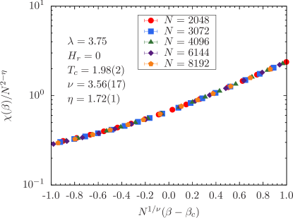
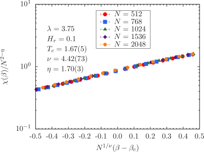
Figure 4: (Color online) Finite-size scaling analysis of $\chi/{N^{2-\eta}}$ as a function of $N^{1/\nu}(\beta-\beta_{c})$ for an Ising spin glass on a scale-free network with Gaussian disorder and $\lambda=3.75$. The data at zero field (top panel) scale very well. The bottom panel shows representative data for $H_{r}=0.1$ scaled according to Eq. (7). Error bars are smaller than the symbols.

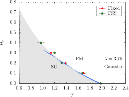
Figure 5: (Color online) Field $H_{r}$ versus temperature $T$ phase diagram for an Ising spin glass on a scale-free graph with $\lambda=3.75$. The data points separate a paramagnetic (PM) from a spin-glass (SG) state. The shaded area is intended as a guide to the eye. The dotted (blue) line is a calculation of the AT line in the $H_{r}\to 0$ limit. Note that estimates for the critical temperature $T_{c}$ from a finite-size scaling analysis (FSS) according to Eq. (7) with $T_{c}$, $\eta$, and $\nu$ as free parameters agree within error bars with estimates at finite fields where $\eta=19/11$ and $\nu=11/3$ are used as fixed parameters (labeled with “Fixed” in the plot).

Table 2: Critical parameters $T_{c}$, $\nu$, and $\eta$ for a spin glass with Gaussian random bonds defined on a scale-free graph. The data for $\lambda=4.50$ have been determined using the mean-field finite-size scaling expression in Eq. (9). In this case one can, in principle, define $\eta=5/3$ and $\nu=3$, although these should be viewed as parameters placed in Eq. (7) to obtain Eq. (9). For $\lambda=3.75$ we determine the critical parameters using Eq. (7). The starred estimates of $T_{c}$ for $H_{r}>0$ have been determined by using the zero-field estimates of $\eta=19/11$ and $\nu=11/3$ as fixed. Both $T_{c}$ and $T_{c}^{\star}$ agree within error bars, except statistical fluctuations are smaller for $T_{c}^{\star}$ because there are fewer fitting parameters.

$\lambda$	$H_{r}$	$T_{c}$	$T_{c}^{\star}$	$\nu$	$\eta$
$3.75$	$0.0$	$1.98(2)$	$1.97(1)$	$3.56(17)$	$1.72(1)$
$3.75$	$0.1$	$1.67(5)$	$1.68(3)$	$4.42(73)$	$1.70(3)$
$3.75$	$0.2$	$1.32(8)$	$1.39(5)$	$6.53(61)$	$1.72(2)$
$3.75$	$0.3$	$1.20(6)$	$1.16(4)$	$3.31(32)$	$1.74(2)$
$3.75$	$0.4$	$0.97(7)$	$1.00(4)$	$3.68(46)$	$1.72(2)$
$4.50$	$0.0$	$1.39(1)$		$3$	$5/3$
$4.50$	$0.1$	$1.03(3)$		$3$	$5/3$
$4.50$	$0.2$	$0.66(5)$		$3$	$5/3$
$4.50$	$0.3$	$0.55(5)$		$3$	$5/3$
$4.50$	$0.4$	$0.46(4)$		$3$	$5/3$

IV Nonequilibrium properties in a field

It has recently been shown that a key ingredient for the existence of SOC in glassy spin systems is a diverging number of neighbors Andresen et al. (2013). Scale-free networks have a power-law degree distribution. If the exponent $\lambda\leq 2$, then scale-free networks have an average number of neighbors $K$ that diverges with the system size. Therefore, it is possible that SOC might be present in this regime. To test this prediction, in this section we compute nonequilibrium avalanche distributions of spin flips driven by an external field.

IV.1 Numerical details and measured observables

We study the Hamiltonian in Eq. (2) either with Gaussian [Eq. (4)] or bimodal [Eq. (5)] disorder. The external magnetic field used to drive the avalanches is uniform rather than drawn from a Gaussian distribution, i.e., $H_{i}=H$ in Eq. (2). Spin-flip avalanches are triggered by using zero-temperature Glauber dynamics Sethna et al. (1993); Perkovic et al. (1999); Katzgraber et al. (2002); Andresen et al. (2013). In this approach one computes the local fields

$$h_{i}=\sum_{j}{J_{ij}}{S_{j}}-H$$ (15)

felt by each spin. A spin is unstable if the stability $h_{i}S_{i}<0$ is negative. The initial field $H$ is selected to be larger than the largest local field, i.e., $H>|h_{i}|$ $\forall i$. Furthermore, we set all spins $S_{i}=+1$. The spins are then sorted by local fields and the field $H$ reduced until the stability of the first sorted spin is negative, therefore making the spin unstable. This (unstable) spin is flipped, then the local fields of all other spins updated, and the most unstable spin is flipped again until all spins are stable, i.e., the avalanche ends. Simulation parameters are shown in Table 3.

Table 3: Simulation parameters in the nonequilibrium study with both Gaussian and bimodal-distributed random bonds: For each exponent $\lambda$ we study systems of $N=500\times 2^{m}$ spins with $m\in\{1,\ldots,m_{\rm max}\}$. For Gaussian disorder, when $\lambda<4$, we also simulate systems with $48\,000$ spins ($m=6$ corresponds to $32\,000$ spins). All distributions are computed using $N_{\rm sa}$ disorder realizations.

disorder type	$\lambda$	$m_{\rm max}$	$N_{sa}$
Gaussian	$1.50$	$6$	$12\,000$
Gaussian	$2.00$	$6$	$12\,000$
Gaussian	$2.50$	$6$	$12\,000$
Gaussian	$3.00$	$6$	$12\,000$
Gaussian	$3.50$	$6$	$12\,000$
Gaussian	$4.00$	$5$	$12\,000$
Gaussian	$4.50$	$5$	$12\,000$
Gaussian	$5.00$	$5$	$12\,000$
Gaussian	$5.50$	$5$	$12\,000$
Gaussian	$6.00$	$4$	$12\,000$
Gaussian	$6.50$	$4$	$12\,000$
Gaussian	$7.00$	$4$	$12\,000$
Bimodal	$1.50$	$6$	$12\,000$
Bimodal	$2.00$	$6$	$12\,000$
Bimodal	$2.25$	$6$	$12\,000$
Bimodal	$2.50$	$6$	$12\,000$
Bimodal	$3.00$	$6$	$12\,000$
Bimodal	$3.50$	$6$	$12\,000$
Bimodal	$4.00$	$6$	$12\,000$
Bimodal	$4.50$	$5$	$12\,000$
Bimodal	$5.00$	$5$	$12\,000$

We measure the number of spins that flipped until the system regains equilibrium and record the avalanche size distributions $D(n)$ for all triggered avalanches of size $n$ until $S_{i}\rightarrow-S_{i}$ $\forall i$. When SOC is present (as for the SK model), we expect the avalanche distributions to be power-law distributed with an exponential cutoff that sets in at a characteristic size $n^{*}$. Only if $n^{*}(N)\to\infty$ for $N\to\infty$ without tuning any parameters does the system exhibit true SOC. $n^{*}$ is determined by fitting the tail of the distributions to $D(n)\sim\exp[-n/n^{*}(N)]$ with $n^{*}(N)$ a fitting parameter. This procedure is repeated for different values of $\lambda$ and the thermodynamic value of $n*$ is determined by an extrapolation in the system size $N$.

IV.2 Numerical results for Gaussian disorder

We start by showing avalanche distributions for selected values of the exponent $\lambda$ which show the characteristic behavior of the system.

Figure 6 (top panel) shows avalanche distributions $D(n)$ for $\lambda=4.50$ recorded across the whole hysteresis loop (bottom panel). Here, the number of neighbors does not diverge with the system size because $\lambda=4.50>2$. The distributions show no system size dependence. The fact that the data show a curvature in a log-log plot clearly indicate that these are not power laws. Although tens of thousands of spins are simulated, the largest avalanches found span less than 1% of the system. The vertical line represents the extrapolated typical avalanche size $n^{*}$ which is rather small and indicates that the system is not in an SOC state.

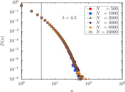
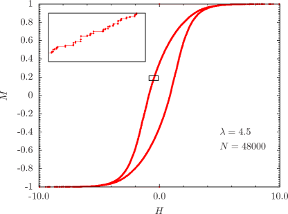
Figure 6: (Color online) Top: Avalanche distribution $D(n)$ for the Edwards-Anderson spin-glass model with Gaussian disorder on scale-free networks with $\lambda=4.50$ recorded across the whole hysteresis loop. The data show no system size dependence. The vertical (black) line marks the extrapolated value of $n^{*}$. Clearly, no signs of SOC are visible in the data. Bottom: Magnetization $M=(1/N)\sum_{i}s_{i}$ versus field $H$ hysteresis loop for $\lambda=4.50$ and $48000$ spins. The data are for one single sample and meant as an illustration for the typical behavior of the system in a field. The inset shows a zoom into the boxed region. The discrete steps due to magnetization jumps in the hysteresis loop are clearly visible.

In contrast, Fig. 7, top panel, shows data for $\lambda=1.5<2$ in the regime where the number of neighbors diverges with the system size. The distributions $D(N)$ have a clearly visible power-law behavior with a crossover size $n^{*}(N)$ that grows with increasing system size. Furthermore, a careful extrapolation to the thermodynamic limit shows that $1/n^{*}=-0.0012(23)$, i.e., $n^{*}=\infty$. The hysteresis loop shown in the bottom panel of Fig. 7 suggests that for this value of $\lambda$ larger rearrangements of spins are possible.

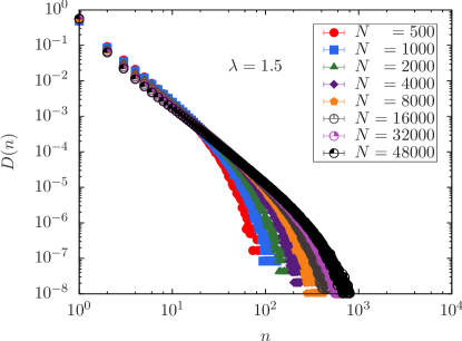
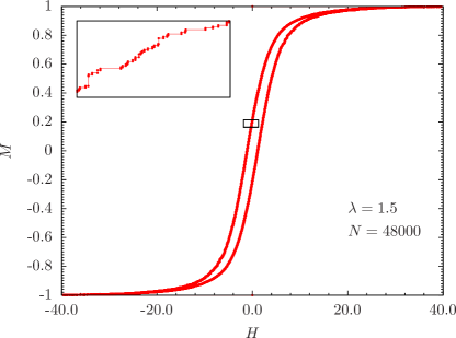
Figure 7: (Color online) Top: Avalanche distribution $D(n)$ for the Edwards-Anderson spin-glass model with Gaussian disorder on scale-free networks with $\lambda=1.5$ recorded across the whole hysteresis loop. For $\lambda=1.5<2.0$ the number of neighbors diverges. The data show a clear system-size dependence with the distributions becoming increasingly power-law-like for increasing system size $N$. As shown in Fig. 8, the extrapolated cutoff value is $n^{*}=\infty$, i.e., the system exhibits true SOC behavior. Bottom: Magnetization $M=(1/N)\sum_{i}s_{i}$ versus field $H$ hysteresis loop for $\lambda=1.50$ and $48000$ spins. The data are for one single sample and meant as an illustration for the typical behavior of the system in a field. The inset shows a zoom into the boxed region. The discrete steps due to magnetization jumps in the hysteresis loop are clearly visible. Qualitatively, the data seem to show larger rearrangements as for $\lambda=4.50$ (Fig. 6).

We have repeated these simulations for several values of the exponent $\lambda$. Our results are summarized in Fig. 8, where $1/n^{*}$ is plotted as a function of $\lambda$. Clearly, $1/n^{*}=0$ only if $\lambda\leq 2$, i.e., in the regime where the number of neighbors diverges, in perfect agreement with the results of Ref. Andresen et al. (2013) for hypercubic systems, as well as the SK model Pázmándi et al. (1999). Note that we have also recorded distributions of magnetization jumps (not shown) Pázmándi et al. (1999); Andresen et al. (2013) that qualitatively display the same behavior as the avalanche size distributions.

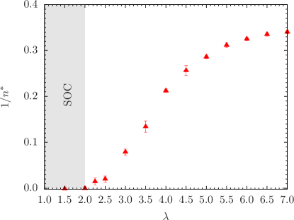
Figure 8: (Color online) Characteristic avalanche size $n^{*}$ extrapolated to the thermodynamic limit for different values of $\lambda$ and Gaussian disorder. Plotted are $1/n^{*}$ versus $\lambda$. Only when $1/n^{*}=0$ (here within error bars) we can expect the system to show SOC behavior. This is only the case for $\lambda\leq 2$, i.e., in the regime where the number of neighbors diverges.

IV.3 Numerical results for bimodal disorder

So far, we have only probed for the existence of SOC within the spin-glass phase. Bimodal disorder [Eq. (5)] has the advantage that one can easily tune the fraction of ferromagnetic bonds by changing $p$. When $p=1$ the system is a pure ferromagnet, whereas for $p=0$ it is an antiferromagnet and for $p=0.5$ a spin glass (comparable to the Gaussian case).

Sethna et al., as well as others, have studied the random-field Ising model Imry and Ma (1975); Sethna et al. (1993); Vives and Planes (1994); Perkovic et al. (1995, 1999); Kuntz et al. (1998); Sethna et al. (2004) where the level of ferromagnetic behavior is tuned by changing the width of the random-field distribution $\sigma$. In particular, for three space dimensions, there is a critical value $\sigma_{c}$ where a jump in the hysteresis loop appears, i.e., large system-spanning rearrangements of the spins start to occur when $\sigma>\sigma_{c}$. We call this regime supercritical because here system-spanning avalanches will always occur in a predominant fashion. For $\sigma=\sigma_{c}$ true power-law distributions of the spin avalanches are obtained, whereas for $\sigma<\sigma_{c}$ no system-spanning rearrangements are found. We call the latter scenario subcritical.

Here we find a similar behavior when tuning the fraction of ferromagnetic bonds $p$. Figure 9 shows the typical behavior we observe for the avalanche distributions $D(n)$. For $p=0.63$ and $\lambda=3.50$ (Fig. 9, top panel), the distributions show small system-size dependence. A detailed analysis of the characteristic avalanche size $n^{*}(N)$ shows that it extrapolates to a finite value in the thermodynamic limit. This means we are in the subcritical regime. However, for $\lambda=3.50$ and $p=0.66$ clear power laws in the distributions $D(n)$ emerge (Fig. 9, center panel). Here $n^{*}\to\infty$, i.e., true power-law behavior. However, for $\lambda=3.50$ and $p=0.70$, although most of the distributions show a clear power-law-like behavior, a bump for large $n$ appears (Fig. 9, bottom panel). In this case the probability for very large rearrangements increases. Direct inspection of the underlying hysteresis loops (not shown) shows a jump in the magnetization, i.e., we are in the supercritical regime. We repeat these simulations for different exponents $\lambda$ and vary the fraction of ferromagnetic bonds $p$ until the distributions are power laws. This allows us to construct the phase diagram shown in Fig. 10. We find a critical line $p_{c}(\lambda)$ (triangles, solid curve) that separates the subcritical region from the supercritical region. Along the critical line avalanche size distributions are power laws. Note that this critical line shows no close correlations with the spin-glass–to–ferromagnetic boundary computed in Ref. Katzgraber et al. (2012) (dotted line in Fig. 10). For $\lambda\leq 2$ and when $p=0.5$, i.e., within the spin-glass phase where the graph connectivity diverges, we recover true SOC.

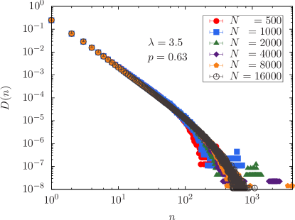
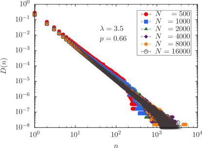
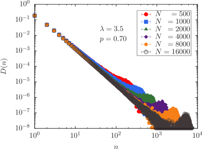
Figure 9: (Color online) Avalanche distribution $D(n)$ for the Edwards-Anderson spin-glass model with bimodal disorder on scale-free networks with $\lambda=3.5$ recorded across the whole hysteresis loop. Top panel: Data for $p=0.63<p_{c}$. Here the system displays subcritical behavior, i.e., the characteristic avalanche size $n^{*}$ is finite. Center panel: For $p=0.66\approx p_{c}$ the system is in the critical regime where the distributions are well described by power laws. Bottom panel: For $p=0.70>p_{c}$ the system is in the supercritical regime. A jump in the hysteresis loop occurs, i.e., very large rearrangements are very probable, as can be seen in the bump that develops in the distributions $D(n)$ for large $n$.

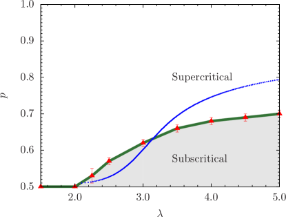
Figure 10: (Color online) Fraction of ferromagnetic bonds $p$ versus $\lambda$ phase diagram for the Edwards-Anderson spin-glass model on scale free networks with bimodal interactions between the spins. For $\lambda>2$ a critical line $p_{c}(\lambda)$ separates the subcritical regime where avalanches are small, from the supercritical regime where system-spanning avalanches are very common. Along the critical line $p_{c}(\lambda)$ (triangles, solid line) avalanche sizes are distributed according to power laws. For $\lambda\leq 2$ the number of neighbors diverges. In this regime for $p=0.5$ the system displays avalanches that are power laws, i.e., true SOC. The dotted line represents the spin-glass–to–ferromagnetic phase boundary from Fig. 2 in Ref. Katzgraber et al. (2012).

V Summary and Conclusions

We have studied Boolean (Ising) variables on a scale-free graph with competing interactions in an external field both in thermal equilibrium, as well as in a nonequilibrium hysteretic setting.

At finite temperatures, we show that for $\lambda>3$, where at zero field the system orders at finite temperatures Katzgraber et al. (2012), spin glasses on scale-free graphs do order in a field, i.e., their behavior is very much reminiscent of the mean-field SK model in a field. Naively, one could have expected that outside the SK regime ($\lambda<4$) a behavior reminiscent of (diluted) one-dimensional spin glasses with power-law interactions Kotliar et al. (1983); Katzgraber and Young (2003); Leuzzi et al. (2008) emerges where a spin-glass state in a field seems stable only within the mean-field regime of the model Katzgraber and Young (2005); Katzgraber et al. (2009). These results again illustrate the superb robustness of Boolean decision problems on scale-free networks to perturbations. In this case, a stable spin-glass state emerges at nonzero temperatures even in the presence of magnetic fields (external global biases).

At zero temperature, when driven with an external field, Boolean decision problems on scale-free networks show self-organized critical behavior only when the number of neighbors diverges with the system size, i.e., for $\lambda\leq 2$. For $\lambda>2$ and with bimodal disorder, a behavior reminiscent of the random-field Ising model is found Sethna et al. (1993); Vives and Planes (1994); Perkovic et al. (1995, 1999); Kuntz et al. (1998); Sethna et al. (2004) where system-spanning avalanches only occur whenever the fraction of ferromagnetic bonds $p_{c}(\lambda)$ is tuned towards a critical value. These results show that “damage” can easily spread on real networks where typically $\lambda\lesssim 3$. Therefore, in contrast the robustness found at finite temperatures, Boolean decision problems on scale-free networks show a potential fragility when driven in a nonequilibrium scenario at zero temperature.

It will be interesting to perform these simulations for real networks in the future, as well as the study of $q$-state Potts variables Yeomans (1992).

*

Appendix A Analytical form of the de Almeida-Thouless for $H_{r}\to 0$

In this appendix we derive analytically the form of the AT line in the limit when $H_{r}\to 0$ for a type of scale-free network which is very convenient for analytical calculations, namely the static model used by Kim et al. Kim et al. (2005), whose procedures and equations we shall closely follow. In this model the number of vertices $N$ is fixed. Each vertex $i$ ($i=1,2,\ldots,N$) is given a weight $p_{i}$, where

$$p_{i}=\frac{i^{-\mu}}{\zeta_{N}(\mu)}.$$ (16)

where $\mu$ is related to $\lambda$ via $\lambda=1+1/\mu$, and

$$\zeta_{N}(\mu)\equiv\sum_{j=1}^{N}j^{-\mu}\approx\frac{N^{1-\mu}}{1-\mu}.$$ (17)

Only $\mu$ in the range $[0,1)$ (i.e., $\lambda>2$) will be discussed. Two vertices $i$ and $j$ are selected with probabilities $p_{i}$ and $p_{j}$ and if $i\neq j$ they are connected with a single bond unless the pair are already connected. The process is repeated $NK/2$ times. Then in such a network, the probability that a given pair of vertices is not connected by an edge is $1-f_{ij}=(1-2p_{i}p_{j})^{NK/2}\approx\exp(-NKp_{i}p_{j})$, and the probability that they are connected by an edge is $f_{ij}=NKp_{i}p_{j}$. This product form for $f_{ij}$ enabled Kim et al. Kim et al. (2005) to proceed analytically. Note that here $K$ is the mean degree of the scale-free network generated by this procedure.

We shall work in the paramagnetic phase where the spin glass is replica symmetric, i.e., where

$$q_{ab}=\sum_{i}p_{i}\langle s_{i}^{a}s_{i}^{b}\rangle=q,$$ (18)

independently of the replica labels $a=1,2,\ldots,n$, where $n$ is set to zero at the end of the calculation. In $q_{ab}$, $a\neq b$. Kim et al. Kim et al. (2005) showed then that the higher order parameters such as $q_{abcd}=\sum_{i}p_{i}\langle s_{i}^{a}s_{i}^{b}s_{i}^{c}s_{i}^{d}\rangle$ can be neglected when $q$ is sufficiently small—that is, in the region near $T_{c}$ studied in this appendix—and that a “truncation” approximation can be made for $q$

$$q=\int{\cal D}z\sum_{i=1}^{N}p_{i}\tanh^{2}\left(z\sqrt{NK{\bf T}_{2}p_{i}q+H_{r}^{2}/T^{2}}\right),$$ (19)

where

$$\int{\cal D}z\equiv\frac{1}{\sqrt{2\pi}}\int_{-\infty}^{\infty}dze^{-z^{2}/2}$$ (20)

and

$${\bf T}_{2}=\langle\tanh^{2}(J_{ij}/T)\rangle.$$ (21)

Here the average is over the distribution of bonds, assumed symmetric, i.e., $P(J_{ij})=P(-J_{ij})$. The random field of variance $H_{r}^{2}$ was not included in the Kim et al. Kim et al. (2005) paper, but Eq. (19) is consistent with the equations for a spin glass in a random field studied in Ref. Sharma and Young (2010) (in the appropriate limit).

In the $H_{r}$–$T$ phase diagram it is expected that the assumption of replica symmetry holds until the AT line is crossed. The equation of the line where the spin-glass susceptibility diverges follows from the expressions given in Ref. Kim et al. (2005):

$$(K{\bf T}_{2})^{-1}=\int\!\!{\cal D}z\sum_{i=1}^{N}Np_{i}^{2}{\rm sech}^{4}\left(z\sqrt{NK{\bf T}_{2}p_{i}q+H_{r}^{2}/T^{2}}\right).$$ (22)

The solution of Eqs. (19) and (22) together fix the equation of the AT line.

It is convenient to convert the sums over $i$ to integrals. Let $x=i/N$. Then $\sum_{i=1}^{N}\to\int_{0}^{1}Ndx$, and in the large-$N$ limit Eq. (19) becomes

$$q=\int{\cal D}z\int_{0}^{1}dx\frac{1-\mu}{x^{\mu}}\tanh^{2}\left(z\sqrt{Q^{\prime}/x^{\mu}+H_{r}^{2}/T^{2}}\right),$$ (23)

where $Q^{\prime}=(1-\mu)K{\bf T}_{2}q$. Equation (22) becomes on converting the sum to an integral

$$(K{\bf T}_{2})^{-1} = \int{\cal D}z\int_{0}^{1}dx\frac{(1-\mu)^{2}}{x^{2\mu}}$$ (24)

$$\;\;\;\;\;\;\;{\rm sech}^{4}\left(z\sqrt{Q^{\prime}/x^{\mu}+H_{r}^{2}/T^{2}}\right).$$

We shall only study explicitly here the case where $3<\lambda<4$ ($1/3<\mu<1/2$). Similar procedures can be used to determine the AT line when $\lambda>4$. We first rewrite Eq. (23) as

$$q=\int{\cal D}z\int_{0}^{1}dx\frac{1-\mu}{x^{\mu}}\left\{z^{2}(Q^{\prime}/x^{\mu}+H_{r}^{2}/T^{2})+\left[\tanh^{2}\left(z\sqrt{Q^{\prime}/x^{\mu}+H_{r}^{2}/T^{2}}\right)-z^{2}(Q^{\prime}/x^{\mu}+H_{r}^{2}/T^{2})\right]\right\}.$$ (25)

The integral over $z$ involving just the first line of Eq. (25) can be done to yield

$$q=(K/K_{p}){\bf T}_{2}q+H_{r}^{2}/T^{2}+R(H_{r},q),$$ (26)

where

$$K_{p}=\frac{1-2\mu}{(1-\mu)^{2}},$$ (27)

and

$$R(H_{r},q)=\int{\cal D}z\int_{0}^{1}dx\frac{1-\mu}{x^{\mu}}\left[\tanh^{2}\left(z\sqrt{Q^{\prime}/x^{\mu}+H_{r}^{2}/T^{2}})-z^{2}(Q^{\prime}/x^{\mu}+H_{r}^{2}/T^{2}\right)\right].$$ (28)

One can show that $R(H_{r},q)=R(0,q)+{\mathcal{O}}(Q^{\prime}H_{r}^{2}/T^{2})$. For small $q$, the term in addition to $R(0,q)$ is negligible in comparison to the term $H_{r}^{2}/T^{2}$ in Eq. (26) and can be dropped. We next re-write the integral for $R(0,q)$ as

$$R(0,q)=\int{\cal D}z\left(\int_{0}^{\infty}dx-\int_{1}^{\infty}dx\right)\frac{1-\mu}{x^{\mu}}\big{[}\tanh^{2}(z\sqrt{Q^{\prime}/x^{\mu}})-z^{2}Q^{\prime}/x^{\mu}\big{]}.$$ (29)

The integral from $1$ to $\infty$ can be evaluated for small $Q^{\prime}$ by expanding the $\tanh$ in a power series in $Q^{\prime}$. The integrals converge for $\lambda<4$ and the leading contribution is

$$2{Q^{\prime}}^{2}(1-\mu)\frac{\lambda-1}{4-\lambda}+{\mathcal{O}}({Q^{\prime}}^{3}).$$

The integral from $0$ to $\infty$ can by evaluated after a variable change $w=z\sqrt{Q^{\prime}/x^{\mu}}$ when it gives a contribution $F(\lambda){Q^{\prime}}^{\lambda-2}$, where

$$F(\lambda)=P(\lambda)\int_{0}^{\infty}dw\,w^{3-2\lambda}[\tanh^{2}w-w^{2}].$$ (30)

Here $P(\lambda)=(1-\mu)\Gamma(\lambda-3/2)2^{\lambda-1}(\lambda-1)/\sqrt{\pi}$. Thus, for $3<\lambda<4$, the equation of state is

$$H_{r}^{2}/T^{2} = q[1-K{\bf T}_{2}/K_{p}]-F(\lambda){Q^{\prime}}^{\lambda-2}$$ (31)

$$\;\;-2{Q^{\prime}}^{2}(1-\mu)\frac{\lambda-1}{4-\lambda}+{\mathcal{O}}({Q^{\prime}}^{3}),$$

which agrees with the expression given in Ref. Kim et al. (2005) when $H_{r}=0$.

When $4<\lambda<5$, one can proceed in a similar fashion. The equation of state is unchanged except $F(\lambda)$ becomes $\tilde{F}(\lambda)$ where

$$\tilde{F}(\lambda)=P(\lambda)\int_{0}^{\infty}dw\,w^{3-2\lambda}[\tanh^{2}w-w^{2}+2w^{4}/3].$$ (32)

For $\lambda>5$ the term in ${Q^{\prime}}^{\lambda-2}$ is subdominant to the term of order ${Q^{\prime}}^{3}$ and can be ignored to leading order.

We next deduce some simple features which follow from the equations of state. In the high-temperature state $q\sim H_{r}^{2}/T^{2}$, and in the limit of $H_{r}/T\to 0$,

$$\chi_{SG}\to\frac{q}{(H_{r}^{2}/T^{2})}=\frac{1}{1-K{\bf T}_{2}/K_{p}}.$$ (33)

The zero-field spin-glass susceptibility $\chi$ diverges at the zero-field transition temperature $T_{c}$ where ${\bf T}_{2}=K_{p}/K$, and at lower temperatures $q$ becomes nonzero. The divergence of this susceptibility as the transition is approached is of the same form for all $\lambda>3$. This means for the critical exponent

$$\gamma=1\;\;\;\;\;\;\;\;\;\;\;\;\;\;\;\;\;\;\;\;\;\;\;\;\;\;\;\;(\lambda>3)$$ (34)

However, the exponent $\beta$ in $q\sim(1-T/T_{c})^{\beta}$ depends on $\lambda$. We obtain

$$\beta = \frac{1}{\lambda-3}\;\;\;\;\;\;\;\;\;\;\;\;\;\;\;\;\;(3<\lambda<4)$$ (35)

$$\beta = 1\;\;\;\;\;\;\;\;\;\;\;\;\;\;\;\;\;\;\;\;\;\;\;\;(\lambda>4).$$ (36)

We can use Eq. (24) in conjunction with the equations of state to determine the form of the AT line as $H_{r}/T\to 0$. Once again, we shall start in the region $3<\lambda<4$ and write the term ${\rm sech}^{4}(z\sqrt{Q^{\prime}/x^{\mu}+H_{r}^{2}/T^{2}})$ as $1+[{\rm sech}^{4}(z\sqrt{Q^{\prime}/x^{\mu}+H_{r}^{2}/T^{2}})-1]$. The term in unity in the integral evaluates to $1/K_{p}$, so

$$(K{\bf T}_{2})^{-1}=1/K_{p}+S(H_{r},q),$$ (37)

where

$$S(H_{r},q)=\int{\cal D}z\int_{0}^{1}dx\frac{(1-\mu)^{2}}{x^{2\mu}}\left[{\rm sech}^{4}\left(z\sqrt{Q^{\prime}/x^{\mu}+H_{r}^{2}/T^{2}}\right)-1\right].$$ (38)

Once again, it is sufficient to evaluate $S(H_{r},q)$ at $H_{r}=0$; the corrections of ${\mathcal{O}}(H_{r}^{2}/T^{2})$ are negligible compared to the terms which we retain. Next we rewrite the integral as

$$S(0,q)=\int{\cal D}z\left(\int_{0}^{\infty}dx-\int_{1}^{\infty}dx\right)\frac{(1-\mu)^{2}}{x^{2\mu}}\left[{\rm sech}^{4}\left(z\sqrt{Q^{\prime}/x^{\mu}}\right)-1\right].$$ (39)

The integral from $0$ to $\infty$ can be evaluated after making the same variable change $w=z\sqrt{Q^{\prime}/x^{\mu}}$, when it gives the contribution $G(\lambda){Q^{\prime}}^{\lambda-3}$, where

$$G(\lambda)=2^{\lambda-2}(1-\mu)^{2}(\lambda-1)\Gamma(\lambda-5/2)/\sqrt{\pi}\\ \times\int_{0}^{\infty}dw\,w^{5-2\lambda}[{\rm sech}^{4}w-1].$$

The integral from $1$ to $\infty$ can be done in a power series in $Q^{\prime}$ and the leading term of this contribution to $S(0,q)$ is

$$-2(1-\mu)^{2}Q^{\prime}/(1-3\mu)+{\mathcal{O}}({Q^{\prime}}^{2}).$$

We can now calculate the AT line: It is simplest to combine Eqs. (31) and (37) to eliminate the term in $(1-K{\bf T_{2}}/K_{p})$ when one finds that

$$H_{\rm AT}^{2}/T^{2}=C(\lambda){Q^{\prime}}^{\lambda-2}+{\mathcal{O}}({Q^{\prime}}^{3}),$$ (40)

where

$$C(\lambda)=\frac{1}{\sqrt{\pi}}2^{\lambda-2}(\lambda-2)\Gamma(\lambda-5/2)\int_{0}^{\infty}dw\,w^{5-2\lambda}\left\{{\rm sech}^{4}w-1-2(\lambda-5/2)\left[\tanh^{2}w/w^{2}-1\right]\right\}.$$ (41)

The integral has to be done numerically but it stays finite as $\lambda\to 4$. For example, $C(3.75)\approx 0.530$. The terms of ${\mathcal{O}}({Q^{\prime}}^{2})$ cancel from Eq. (40). Thus, in the range $3<\lambda<4$, the equation of the AT line in terms of the temperature rather than $Q^{\prime}$ is just

$$H_{\rm AT}^{2}/T^{2}\sim(1-T/T_{c})^{\frac{\lambda-2}{\lambda-3}}\;\;\;\;\;\;\;\;\;\;(3<\lambda<4).$$ (42)

Note that this is in agreement with the scaling form

$$H_{\rm AT}^{2}/T^{2}\sim(1-T/T_{c})^{\beta+\gamma},$$ (43)

on inserting the vales for $\beta=1/(\lambda-3)$ and $\gamma=1$ for $3<\lambda<4$.

In the range $4<\lambda<5$, a similar expression holds for $H_{\rm AT}^{2}/T^{2}$ as in Eq. (40), but $C(\lambda)$ becomes $\tilde{C}(\lambda)$ where

$$\tilde{C}(\lambda)=\frac{1}{\sqrt{\pi}}2^{\lambda-2}(\lambda-2)\Gamma(\lambda-5/2)\int_{0}^{\infty}dw\,w^{5-2\lambda}\left\{{\rm sech}^{4}w-1+2w^{2}-2(\lambda-5/2)\left[\tanh^{2}w/w^{2}-1+2w^{2}/3\right]\right\}.$$ (44)

Because in this range the exponent $Q^{\prime}\sim(1-T/T_{c})$, the form of the AT line is

$$H_{\rm AT}^{2}/T^{2}\sim(1-T/T_{c})^{\lambda-2}\;\;\;\;\;\;\;\;\;\;(4<\lambda<5).$$ (45)

Finally, in the range $\lambda>5$, the term in ${Q^{\prime}}^{\lambda-2}$ is subdominant compared with the term in ${Q^{\prime}}^{3}$ and

$$H_{\rm AT}^{2}/T^{2}\sim(1-T/T_{c})^{3}\;\;\;\;\;\;\;\;\;\;(\lambda>5),$$ (46)

which is the familiar form of the AT line in the SK model.

One can also use the static model to investigate the behavior when $\lambda<3$. The spin-glass phase with broken replica symmetry exists in zero field up to infinite temperature, i.e., $T_{c}$ is infinite when $\lambda<3$ Kim et al. (2005). However, in the interval $5/2<\lambda<3$ the application of a large enough random field $H_{r}$ can restore replica symmetry. By solving Eqs. (23) and (24) it can be shown that this happens at a field $H_{\rm AT}$, where, as before, $\beta^{2}H_{\rm AT}^{2}\sim{Q^{\prime}}^{\lambda-2}$ where

$$H_{\rm AT}\sim T^{\frac{5-2\lambda}{3-\lambda}}\;\;\;\;\;\;\;\;\;\;(2.5<\lambda<3).$$ (47)

for the limit when $T\to\infty$. This phase boundary is, as usual, for the thermodynamic limit when $N\to\infty$. The behavior which would be seen in simulations at finite system size $N$ will be complicated by an unfamiliar finite-size behavior because, for this $\lambda$ range, $T_{c}$ at zero field is infinite. When $\lambda<5/2$ we think that for all $H_{r}$ and $T$ the spin-glass phase has broken replica symmetry and so as a consequence, there will then be no AT line.

References

- Albert et al. (1999) R. Albert, H. Jeong, and A.-L. Barabási, Nature 401, 130 (1999).
- Bartolozzi et al. (2006) M. Bartolozzi, T. Surungan, D. B. Leinweber, and A. G. Williams, Phys. Rev. B 73, 224419 (2006).
- Herrero (2009) C. P. Herrero, Eur. Phys. J. B 70, 435 (2009).
- Lee et al. (2006) S. H. Lee, H. Jeong, and J. D. Noh, Phys. Rev. E 74, 031118 (2006).
- Weigel and Johnston (2007) M. Weigel and D. Johnston, Phys. Rev. B 76, 054408 (2007).
- Mooij and Kappen (2004) J. M. Mooij and H. J. Kappen (2004), (arXiv:cond-mat/0408378).
- Kim et al. (2005) D.-H. Kim, G. J. Rodgers, B. Kahng, and D. Kim, Phys. Rev. E 71, 056115 (2005).
- Ferreira et al. (2010) A. L. Ferreira, J. F. F. Mendes, and M. Ostilli, Phys. Rev. E 82, 011141 (2010).
- Ostilli et al. (2011) M. Ostilli, A. L. Ferreira, and J. F. F. Mendes, Phys. Rev. E 83, 061149 (2011).
- Katzgraber et al. (2012) H. G. Katzgraber, K. Janzen, and C. K. Thomas, Phys. Rev. E 86, 031116 (2012).
- de Almeida and Thouless (1978) J. R. L. de Almeida and D. J. Thouless, J. Phys. A 11, 983 (1978).
- Sherrington and Kirkpatrick (1975) D. Sherrington and S. Kirkpatrick, Phys. Rev. Lett. 35, 1792 (1975).
- Newman and Stein (1994) C. M. Newman and D. L. Stein, Phys. Rev. Lett. 72, 2286 (1994).
- Cieplak et al. (1994) M. Cieplak, A. Maritan, and J. R. Banavar, Phys. Rev. Lett. 72, 2320 (1994).
- Schenk et al. (2002) K. Schenk, B. Drossel, and F. Schwabl, in Computational Statistical Physics, edited by K. H. Hoffmann and M. Schreiber (Springer-Verlag, Berlin, 2002), p. 127.
- Pázmándi et al. (1999) F. Pázmándi, G. Zaránd, and G. T. Zimányi, Phys. Rev. Lett. 83, 1034 (1999).
- Gonçalves and Boettcher (2008) B. Gonçalves and S. Boettcher, J. Stat. Mech. P01003 (2008).
- Andresen et al. (2013) J. C. Andresen, Z. Zhu, R. S. Andrist, H. G. Katzgraber, V. Dobrosavljević, and G. T. Zimanyi, Phys. Rev. Lett. 111, 097203 (2013).
- Sethna et al. (1993) J. P. Sethna, K. Dahmen, S. Kartha, J. A. Krumhansl, B. W. Roberts, and J. D. Shore, Phys. Rev. Lett. 70, 3347 (1993).
- Perkovic et al. (1995) O. Perkovic, K. A. Dahmen, and J. P. Sethna, Phys. Rev. Lett. 75, 4528 (1995).
- Perkovic et al. (1999) O. Perkovic, K. A. Dahmen, and J. P. Sethna, Phys. Rev. B 59, 6106 (1999).
- Kuntz et al. (1998) M. C. Kuntz, O. Perkovic, K. A. Dahmen, B. W. Roberts, and J. P. Sethna (1998), (arXiv:cond-mat/9809122v2).
- Sethna et al. (2004) J. P. Sethna, K. A. Dahmen, and O. Perkovic (2004), (arXiv:cond-mat/0406320v3).
- Vives and Planes (1994) E. Vives and A. Planes, Phys. Rev. B 50, 3839 (1994).
- Vives and Planes (2001) E. Vives and A. Planes, Phys. Rev. B 63, 134431 (2001).
- Katzgraber et al. (2001) H. G. Katzgraber, M. Palassini, and A. P. Young, Phys. Rev. B 63, 184422 (2001).
- Katzgraber et al. (2009) H. G. Katzgraber, D. Larson, and A. P. Young, Phys. Rev. Lett. 102, 177205 (2009).
- Barabasi and Albert (1999) A. L. Barabasi and R. Albert, Science 286, 509 (1999).
- Burda and Krzywicki (2003) Z. Burda and A. Krzywicki, Phys. Rev. E 67, 046118 (2003).
- Boguñá et al. (2004) M. Boguñá, R. Pastor-Satorras, and A. Vespignani, Eur. Phys. J. B 38, 205 (2004).
- Catanzaro et al. (2005) M. Catanzaro, M. Boguñá, and R. Pastor-Satorras, Phys. Rev. E 71, 027103 (2005).
- Young and Katzgraber (2004) A. P. Young and H. G. Katzgraber, Phys. Rev. Lett. 93, 207203 (2004).
- Katzgraber and Young (2005) H. G. Katzgraber and A. P. Young, Phys. Rev. B 72, 184416 (2005).
- Jörg et al. (2008) T. Jörg, H. G. Katzgraber, and F. Krzakala, Phys. Rev. Lett. 100, 197202 (2008).
- Baños et al. (2012) R. A. Baños, A. Cruz, L. A. Fernandez, J. M. Gil-Narvion, A. Gordillo-Guerrero, M. Guidetti, D. Iñiguez, A. Maiorano, E. Marinari, V. Martin-Mayor, et al., Proc. Natl. Acad. Sci. U.S.A. 109, 6452 (2012).
- Baity-Jesi et al. (2013) M. Baity-Jesi, R. Alvarez Baños, A. Cruz, L. A. Fernandez, J. M. Gil-Narvion, Gordillo-Guerrero, D. Iñiguez, A. Maiorano, F. Mantovani, E. Marinari, et al. (2013), (arxiv:cond-mat/1307.4998).
- Binder (1981) K. Binder, Phys. Rev. Lett. 47, 693 (1981).
- Ciria et al. (1993) J. C. Ciria, G. Parisi, F. Ritort, and J. J. Ruiz-Lorenzo, J. Phys. I France 3, 2207 (1993).
- Larson et al. (2013) D. Larson, H. G. Katzgraber, M. A. Moore, and A. P. Young, Phys. Rev. B 87, 024414 (2013).
- Geyer (1991) C. Geyer, in 23rd Symposium on the Interface, edited by E. M. Keramidas (Interface Foundation, Fairfax Station, VA, 1991), p. 156.
- Hukushima and Nemoto (1996) K. Hukushima and K. Nemoto, J. Phys. Soc. Jpn. 65, 1604 (1996).
- Katzgraber et al. (2006) H. G. Katzgraber, M. Körner, and A. P. Young, Phys. Rev. B 73, 224432 (2006).
- Binder and Young (1986) K. Binder and A. P. Young, Rev. Mod. Phys. 58, 801 (1986).
- Katzgraber et al. (2002) H. G. Katzgraber, F. Pázmándi, C. R. Pike, K. Liu, R. T. Scalettar, K. L. Verosub, and G. T. Zimányi, Phys. Rev. Lett. 89, 257202 (2002).
- Imry and Ma (1975) Y. Imry and S.-K. Ma, Phys. Rev. Lett. 35, 1399 (1975).
- Kotliar et al. (1983) G. Kotliar, P. W. Anderson, and D. L. Stein, Phys. Rev. B 27, 602 (1983).
- Katzgraber and Young (2003) H. G. Katzgraber and A. P. Young, Phys. Rev. B 67, 134410 (2003).
- Leuzzi et al. (2008) L. Leuzzi, G. Parisi, F. Ricci-Tersenghi, and J. J. Ruiz-Lorenzo, Phys. Rev. Lett. 101, 107203 (2008).
- Yeomans (1992) J. M. Yeomans, Statistical Mechanics of Phase Transitions (Oxford University Press, Oxford, 1992).
- Sharma and Young (2010) A. Sharma and A. P. Young, Phys. Rev. E 81, 061115 (2010).