Density Functional Theory for Protein Transfer Free Energy

Abstract

We cast the problem of protein transfer free energy within the formalism of density functional theory (DFT), treating the protein as a source of external potential that acts upon the solvent. Solvent excluded volume, solvent-accessible surface area, and temperature-dependence of the transfer free energy all emerge naturally within this formalism, and may be compared with simplified “back of the envelope” models, which are also developed here. Depletion contributions to osmolyte induced stability range from $5$-$10k_{{\tiny B}}T$ for typical protein lengths. The general DFT transfer theory developed here may be simplified to reproduce a Langmuir isotherm condensation mechanism on the protein surface in the limits of short-ranged interactions, and dilute solute. Extending the equation of state to higher solute densities results in non-monotonic behavior of the free energy driving protein or polymer collapse. Effective interaction potentials between protein backbone or sidechains and TMAO are obtained, assuming a simple backbone/sidechain 2-bead model for the protein with an effective 6-12 potential with the osmolyte. The transfer free energy $\delta g$ shows significant entropy: $d(\delta g)/dT\approx 20k_{{\tiny B}}$ for a 100 residue protein. The application of DFT to effective solvent forces for use in implicit-solvent molecular dynamics is also developed. The simplest DFT expressions for implicit-solvent forces contain both depletion interactions and an “impeded-solvation” repulsive force at larger distances.

Keywords: Density functional; Transfer model; Osmolytes; Solvation; Protein folding and stability; Implicit solvent model

1 604-822-8813 1 604-822-5324

1 Introduction

Proteins fold and function in the crowded environment of the cell. Cytosolic proteins must negotiate a complex milieu which in many ways is significantly different than the environment in the test tube: roughly 15% of water molecules are motionally restricted by protein and membrane surfaces ¹; the surrounding solvent is enriched in ions such as Potassium but depleted in Sodium and Chlorine; osmoprotectants such as trehalose and various amino acids are present in significant concentration; numerous membrane surfaces such as the nucleus, ER, and Golgi impose charged substrates for protein interaction; macromolecular agents such as the microtubules, actin, ribosomes, soluble proteins and RNA occupy roughly 30% ($\approx 300\mbox{g/}\ell$) of the cellular volume, and modulate stability ², aggregation propensity ³, and dissociation constants ^{4, 5}.

Non-cytosolic proteins also fold in environments distinct from the test tube as well as the cytosol, particularly with respect to ionic and redox conditions as well as the chaperone complement. Proteins destined for the plasma membrane or extracellular matrix are trafficked by the secratory pathway through the ER and Golgi ⁶. The environments in the ER and cytosol are sufficiently different that the conditions for protein folding are generally mutually exclusive between the two milieu. Folding generally occurs in the lumen of the ER, while function occurs either on the plasma membrane or in the extracellular matrix, which is itself densely occupied by highly charged glycosaminoglycans such as hyaluronan and heparin sulfate—large molecules that may facilitate cellular migration and regulate secreted protein activity. Fibrous proteins such as collagen and fibronectin also occupy the extracellular space, and provide structural rigidity while allowing rapid diffusion of nutrients and signalling metabolites between constituent cells.

The above examples demonstrate the need to correctly account for the effect of the cell environment on protein folding, stability, and function. Accurately accounting for the effects of the cell environment presents a challenge however to both experimental and computational studies. Experimentally, most of what is known about protein folding and stability has resulted from in vitro studies at dilute concentrations, and many questions remain as to how well such results apply to a realistic cell environment. Computationally, including explicit solvent along with a realistic concentration of osmolytes in a box of sufficient size to implement periodic boundary conditions outside the range of an electrostatic cutoff typically increases the number of particles in the simulation by a factor on the order of ten or more ⁷. While this can be done for small proteins such as Trp-cage ⁷, investigating larger proteins generally requires coarse-grained models to keep the computational resources required reasonable ⁸.

Computational studies of crowding on isolated monomeric minimal $\beta$-barrel proteins find that the folding temperature is increased and the folding time decreased ^{9, 10}. However, molecular crowding has been shown in secretory cells to impair protein folding and lead to aggregate formation in the ER ¹¹. It has been estimated that increasing the total intracellular protein concentration by 10% can potentially increase the rate of protein misfolding reactions following a nucleation-polymerization mechanism by a factor or 10 ¹². Consistent with these observations and estimates, another MD folding study of a coarse-grained model of crambin found that the presence of multiple protein copies with a weak inter-protein attractive potential (a more realistic scenario) hindered correct monomeric folding and predisposed the system to aggregation and misfolding ¹³.

The above considerations motivate the creation of computational models, with which we can account for the cellular environment around a protein in an accurate but less computationally expensive way. We begin this paper by reviewing some common methods for calculating the free energy to transfer a molecule from one solvent environment to another. Two of the most common of these are phenomenological continuum approaches and liquid state theory approaches.

The observed linear dependence of the log solubility on the number of CH₂ groups and hence chain length, particularly for long chain saturated fatty acids (decanoic acid and longer), and long-chain aliphatic alcohols (1-butanol and longer), can be taken to indicate a free energy change upon transfer to solvent that scales linearly with either volume or surface area. Historically, surface area has been taken, under the assumption that interactions with the solvent take place at the surface of the molecule in question ^{14, 15}. Then the free energy difference between an amino acid in water and in a solvent with some osmolyte concentration is, for a given configuration, given in terms of the accessible surface area (ASA) of that configuration by the phenomenological expression: $\Delta F=\gamma\cdot\mbox{ASA}+c$, where $\gamma$ is obtained from, eg, a tri-peptide experiment ¹⁶.

The coefficient $\gamma$ depends on the atomic species being transferred. A more refined approach is thus necessary for a protein, wherein the accessible area of the various types of amino acids along with the backbone are treated differently, so that

$$\Delta F=\sum_{i}\gamma_{i}\mbox{ASA}_{i}+c$$ (1)

The $\gamma_{i}$ values are taken to be distinct for polar and non-polar residues, and may even depend on the specific amino acid identity ^{17, 18}.

Recent simulation studies have found significant volume contributions to transfer free energies however ⁸. In these studies, model solvents with no enthalpic interaction (hard sphere solvents) still showed significant transfer free energies, due solely to excluded volume. Volume corrections to the surface area model, computed by scaled particle theory or RISM approaches, have been investigated by several authors ^{19, 20, 21, 22}. As well, Baker and colleagues have found that the inclusion of volume terms (computed by scaled particle particle theory) and dispersion integral terms (computed by Weeks-Chandler-Andersen theory) were essential for an accurate implicit solvent description of atomic- scale nonpolar forces ²³.

Obviously, the phenomenological approach can only approximately capture the effects of the environment, which will include both interaction energies between the osmolytes and the protein, and terms arising from the change in entropy of the osmolyte bath. These techniques, though, are popular ^{24, 25, 26, 27, 28, 16, 29, 30}, computationally cheap to implement, and generalizable to include continuum electrostatic and van der Waals terms to accurately parameterize a given solvent- typically water ^{31, 30}.

Approaches based on liquid state theory generally seek to calculate the correlation function between sites within the protein and some model for a continuous medium surrounding it. One approach to doing this is the reference site interaction model (RISM)³², which defines sites in the protein and the surrounding molecules. Once these sites are defined, the correlation function between them can be determined using the Ornstein-Zernike equation ³³:

$$h(r)=c(r)+\int dr^{\prime}\rho\>c(r^{\prime})h(r^{\prime}-r)$$ (2)

where $h(r)$ is the total correlation function, $c(r)$ the direct correlation function, $\rho$ the solvent density. To solve equation (2), a closure relation is needed, such as the hyper-netted chain (HNC) closure ^{33, 34, 35, 36}:

$$h(r)=\mbox{e}^{-\beta u(r)+h(r)-c(r)}-1$$

or the Kovalenko-Hirata closure ³⁷. Here $u(r)$ is the direct interaction potential between particles. Once correlation functions have been calculated, transfer free energies can be determined through standard methods.

Another liquid state theory approach uses the density functional theory (DFT) developed originally for electronic structure calculations and applies it to condensed classical systems ^{38, 39, 40, 41, 42, 43}. It is noteworthy that Peter Wolynes has made significant contributions to the application of density functional methods in condensed matter systems, primarily through his fundamental studies of glass physics and the glass transition ^{44, 45, 46, 47, 48, 49, 50}, but also in protein folding^{51, 52, 53}. Density functional theory has also been applied to a variety of non-homogenous systems such as associating liquids and polymer nanocomposites ^{54, 55}. Takada and colleagues have used DFT to address crowding effects on the aggregation of proteins, wherein protein concentration is treated as a density field with the whole protein simplified to a sphere ^{56, 57}.

Wolynes’s previous applications of DFT to address problems in disordered condensed matter systems have, along with the other studies mentioned above, inspired us to continue this tradition in chemical physics and his legacy in that context, and consider the application of DFT to protein stability. Here we treat the protein as the source of an external potential, which allows a much more realistic protein model. This approach has certain advantages, which we will return to later.

Liquid state theory approaches have been shown to give solvation densities consistent with values from explicit solvent calculations⁵⁸; and can be refined to arbitrary accuracy by including additional interaction site, three body correlations, and quantum corrections. ^{59, 60, 61, 62, 63} Liquid state theory can be used to determine correlation functions for the constituent atoms within osmolytes as well as osmolytes as whole, so that effects such as orientation of polar solvents can be captured. Liquid state theories are generally much more accurate than phenomenological approaches such as Equation (1) ¹⁶, particularly when discrete molecular aspects of solvation are important. The principle disadvantage is the large computational cost of solving the equations for each configuration. As well, implicit solvation models using continuum electrostatics with optimized parameters (GB/SA) are now capable of obtaining solvation energies typically within $\sim$1 kCal/mol of experimental values for small neutral solutes, while charged solutes tend to show larger errors. ⁶⁴ Nevertheless, GB/SA continuum methods have shown increased utility and widespread use for molecular dynamics simulations ^{31, 30}.

A large body of literature is concerned with calculating the electrostatic response of a continuous media to the insertion of a molecule⁶⁵. This is vitally important in the context of water solvation. In this context, DFT has been applied to the problem of solvation by Borgis and colleagues ^{66, 67}. We became aware of their work only in the late in the stages of preparing this manuscript; our approach is similar at least in spirit to theirs, however we take a more conceptual approach to address much larger protein systems and the effects of osmolyte solutions, and how the DFT framework subsumes many of the notions contained in simplified heuristic models.

The problem we consider in this paper is that of calculating the free energy change upon moving a solute such as a protein from a pure water environment and inserting it into a water and osmolyte environment. 1 illustrates the problem we are considering in the context of the Tanford transfer model for protein folding ⁶⁸; we will return to this diagram several times throughout the paper.

The organization of this paper is as follows. We begin in Section 2 by investigating the expected behavior of the surface and volume contributions to the transfer free energy in a heuristic model. In section 3 we derive the principle equations for the DFT model of the transfer free energy. In section 3.2 - section 5, we consider several examples of how the DFT model can be applied, making connections with the model developed in Section 2. We finally conclude and give our outlook on future directions for this approach.

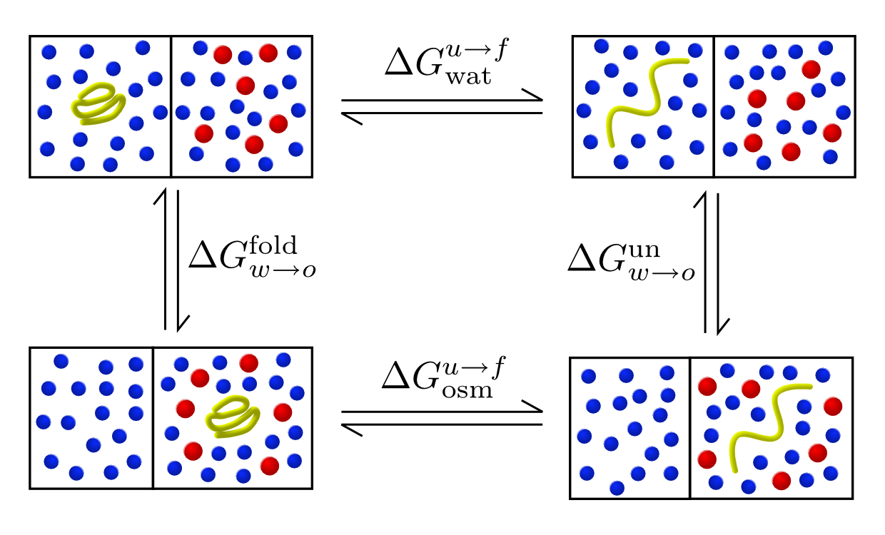
Figure 1: A diagram of the Tanford transfer model, for a transfer process going from a pure water environment to one of water and osmolytes. Knowledge of the free energy of unfolding $\Delta G^{u\rightarrow f}_{\mathrm{wat}}$ in the absence of osmolytes can be combined with the transfer free energies of the folded ($\Delta G^{\mathrm{fold}}_{w\rightarrow o}$) and unfolded ($\Delta G^{\mathrm{un}}_{v\rightarrow s}$) states to obtain the free energy of unfolding in the presence of osmolytes $\Delta G^{u\rightarrow f}_{\mathrm{osm}}$.

2 Volume and Area Terms in the Transfer Free Energy

2.1 Volume Considerations

To appreciate the terms that we expect in an expression for the transfer free energy, we initially consider both volume and surface area effects in a more qualitative way. We consider the difference in volume occupied by the folded and unfolded states, or more precisely the expanded and collapsed states of a polymer, to obtain the corresponding free energy difference in the presence of a bath of “hard-sphere” osmolytes. There are thus no surface interactions to consider, and we seek to estimate the magnitude of the volume effect; we also ignore for the time being the change in internal free energy as the polymer collapses. The free energy change upon collapse of a protein or polymer then arises from the change in entropy of the osmolytes, due to the change in available phase space. For hard-sphere osmolytes, the volume occupied by the expanded polymer will be larger than that of the collapsed polymer. The same considerations apply to a collapsed vs. expanded protein; unfolded states of proteins are generally found to be expanded relative to the folded state ⁶⁹. In what follows, let $r_{a}$ be the mean amino acid radius, $r_{o}$ the osmolyte radius, and $N_{p}$ the number of amino acids in the polymer or protein. Treating the unfolded protein crudely as a meandering cylindrical tube (see 2a inset), the volume is approximately $\pi(r_{a}+r_{o})^{2}(2r_{a}N_{p}+2r_{o})$, which is that of a cylinder of radius $r_{a}+r_{o}$ and length $2N_{p}r_{a}+2r_{o}$. The volume of the collapsed globule, or folded protein, can be modelled as a sphere of radius $R_{p}+r_{o}$, where $R_{p}$ is the protein radius as probed by a zero-radius osmolyte particle, i.e. the collapsed volume is $(4/3)\pi(R_{p}+r_{o})^{3}$. When $r_{o}=0$, the unfolded and folded volumes must be equal, giving $R_{p}^{3}=(3/2)N_{p}r_{a}^{3}$. The change in available volume for osmolytes $\Delta V(r_{o})$ upon polymer collapse is thus positive, and is plotted in 2 as a function of osmolyte radius $r_{o}$, for a chain of length $N_{p}=70$.

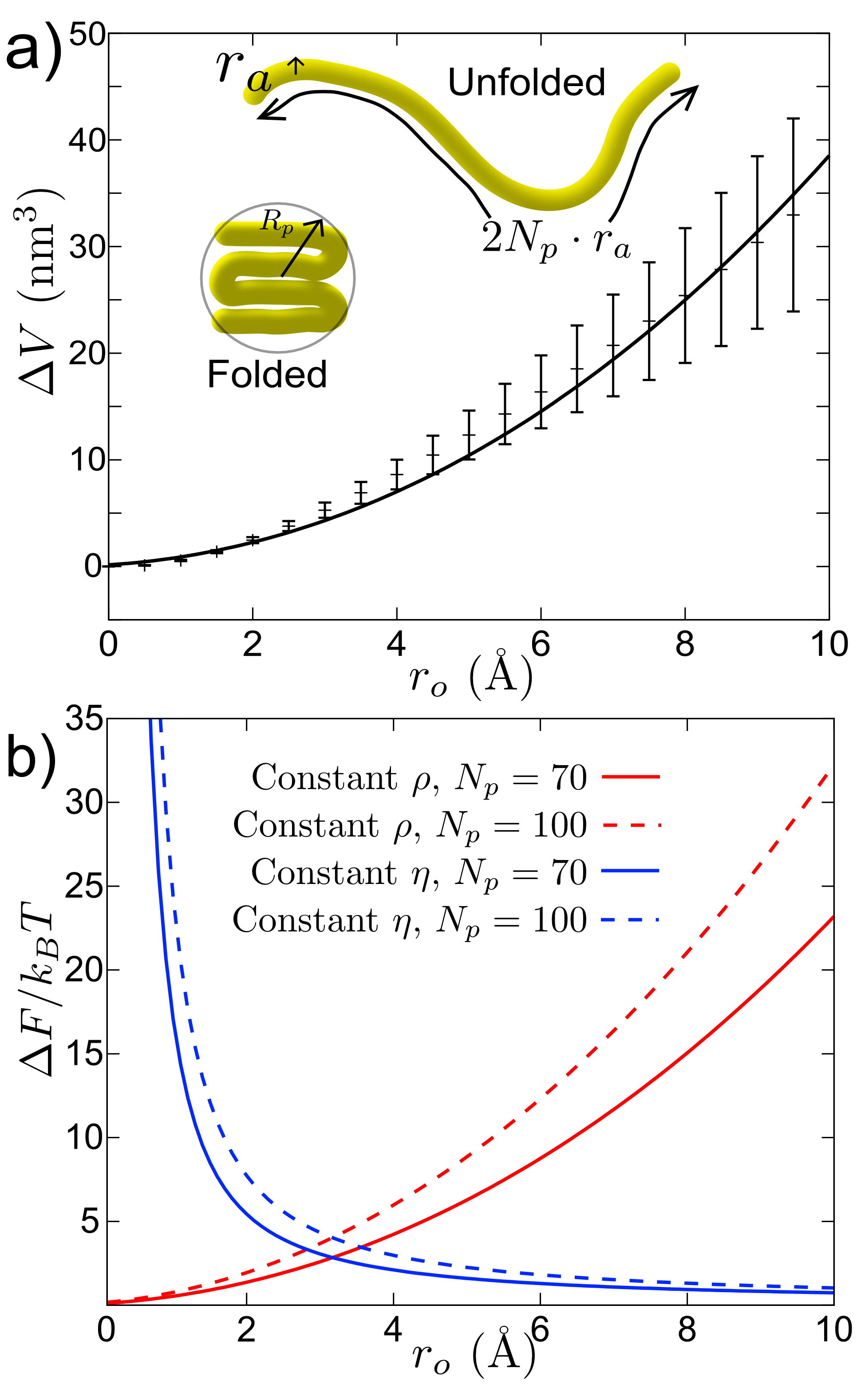
Figure 2: a) Plot of minus the change in volume upon collapse $\Delta V(r_{o})=V_{u}-V_{f}$, as a function of osmolyte radius $r_{o}$, for a polymer chain of length $N_{p}=70$ residues and with $r_{a}=6$ Å. The magnitude of the change in volume monotonically increases as $r_{o}$ increases. Also plotted are the average $\Delta V=\langle V_{u}\rangle-\langle V_{f}\rangle$ values of simulation trajectories of Cold-Shock Protein ($N=70$, PDB 2L15) against probe radius. (Inset) Schematic of collapsed/folded and unfolded polymer. Folded polymer has radius $R_{p}$; unfolded polymer has tube radius $r_{a}$ and length $N_{p}r_{a}$. b) Minus the change in free energy upon collapse as a function of osmolyte radius $r_{o}$, for both constant packing fraction $\eta$ and constant concentration $\rho$. The value of $\rho$ was set to $1M$, and the value of $\eta$ was set so that the free energy change would be equal to that at constant $\rho$ at a typical osmolyte radius of $3.1$ Å. This gave a packing fraction $\eta\approx 0.075$.

We can compare the results of the above simple model to data taken from simulations of a C_α Gō model of cold-shock protein (PDB 2L15), with $70$ amino acids, generated with the GROMACS molecular dynamics package. The Gō potential was generated using a shadow map for the native contacts ⁷⁰ by the SMOG@ctbp server ⁷¹. The simulated free energy surface has a double-well structure with well-defined folded ($f$) and unfolded ($u$) ensemble as observed in C_α Gō models for other single domain proteins ⁷². We take conformational snapshots in each ensemble and measure the volume using a variable probe radius with the program VOIDOO ⁷³. The average volume change $\Delta V=\langle V_{u}\rangle-\langle V_{f}\rangle$ for a given probe radius is plotted in 2a. The theory and simulation data compare quite well given the simplicity of the model.

We now consider the free energy as a function of either uniform density $\rho$ or packing fraction $\eta$ of the osmolytes. Given a large effective box with volume $V_{box}$ containing a given protein, the packing fraction of osmolytes $\eta$ (i.e. the volume density) is given by

$$\eta=\frac{\frac{4}{3}\pi r_{o}^{3}N_{o}}{V_{box}-V_{prot}(r_{o})}\approx\frac{\frac{4}{3}\pi r_{o}^{3}N_{o}}{V_{box}}=\frac{4}{3}\pi r_{o}^{3}\cdot\rho\>,$$

where $\rho$ is the number density. So, at a fixed packing fraction the number of osmolytes $N_{o}$ scales as $r_{o}^{-3}$.

To estimate the volume contributions to the free energy change upon collapse, $\Delta F_{V}(r_{o})$, as a function of osmolyte radius but at either fixed density or packing fraction, we use the ideal gas approximation for the osmotic pressure $p_{osm}=\rho k_{B}T$ to obtain

$$\Delta F_{V}(r_{o})=p_{osm}\Delta V(r_{o})=\rho k_{B}T\Delta V(r_{o})=\frac{\eta k_{B}T\Delta V(r_{o})}{\frac{4}{3}\pi r_{o}^{3}}$$ (3)

where $\Delta V(r_{o})$ is obtained from the model above.

A plot of the magnitude of the free energy change upon collapse as a function of osmolyte radius, here exclusively due to the increase in entropy of osmolyte particles, is shown in 2b. Based on these considerations we can estimate the volume-like contribution for typical osmolyte sizes and concentrations. Taking TMAO as an example, we expect the osmolyte radius to be about 2 Å, from the water oxygen-TMAO nitrogen radial distribution function⁷⁴. Given this radius and a concentration of 300 g/L, for a protein of length $N_{p}=70$ we estimate a volume contribution to the free energy of $\approx 4k_{B}T$. The free energy of unfolding is linear in protein length, so a larger protein of $N_{p}=300$ has an estimated $\Delta G\approx 17k_{B}T$.

2.2 Surface Considerations

The presence of osmolytes in solution can make the effective solvent more repulsive to protein resulting in stabilization, or more attractive to the protein resulting in denaturation. What effect is observed depends on the energy $\epsilon$ of osmolyte-protein binding and also the concentration $c$ (or equivalently the chemical potential $\mu$) of the osmolyte.

The energy $\epsilon$ of binding of the osmolyte is actually the difference in internal free energy of binding between osmolyte and water, since for example water may have some attraction to the polymer, and also an osmolyte may supplant more than one water molecule in the process of binding.

Previous treatments of transfer free energy analysis as a condensation problem onto the surface of the protein have been undertaken primarily in the context of protein denaturation and the prediction of $m$-values ^{75, 76, 77}. The process of condensation of an osmolyte to a surface is equivalent to the well-known statistical mechanical problem of Langmuir’s isotherm ⁷⁸, for which the partition function $\mathfrak{Z}$ in the $(T,\mu)$ ensemble for a substrate with $M$ absorbing sites is given by $\left(1+\mbox{e}^{-\beta\left(\epsilon-\mu\right)}\right)^{M}$. The mean covering ratio $f$ is then given by

$$f=\frac{kT}{M}\frac{\partial\log\mathfrak{Z}}{\partial\mu}=\frac{1}{1+\mbox{e}^{\beta\left(\epsilon-\mu\right)}}\>,$$ (4)

and the mean energy of condensation on the surface is $Mf\epsilon$. Here we neglect interactions between osmolytes when bound. The Helmholtz free energy in this model is given by

$$F=-pV+fM\mu=-k_{B}T\log(\mathfrak{Z})+fM\mu$$

with $T,\mu$ partition function $\mathfrak{Z}$ as given above.

We can relate the Langmuir isotherm to the free energy of a protein surface by assuming that each osmolyte occupies an area $a_{0}\approx\pi r_{o}^{2}$ on the protein surface, so that we can write $M=A/a_{0}$, where $A$ is the protein’s solvent accessible surface area in a given conformation. The change in free energy $F_{A}$ upon condensation becomes

$$F_{A}=-k_{B}T\frac{A}{a_{0}}\log\left(1+\mbox{e}^{-\beta\left(\epsilon-\mu\right)}\right)+f\frac{A}{a_{o}}\mu$$ (5)

If the concentration of unbound osmolyte is dilute, an ideal gas approximation suffices for the chemical potential: $\mu=kT\log\left(\rho/\rho_{Q}\right)$, where $\rho_{Q}$ is a reference concentration (typically taken to be 1M). The quantity $\mathrm{e}^{-\beta\epsilon}/\rho_{Q}$ is typically treated as an equilibrium constant in the literature ^{76, 77}. We consider both dilute and non-dilute limits below. The protein’s exposed surface area is obtained from the volume given in section 2.1 by $A=\partial V/\partial r_{o}$, so the collapsed exposed area is $4\pi\left(R_{p}+r_{o}\right)^{2}$ and the expanded (random coil) exposed area is $2\pi\left(r_{o}+r_{a}\right)\left[\left(2N_{p}+1\right)r_{a}+3r_{o}\right]$.

2.3 Combined surface/volume model for the transfer free energy

We can now write the total free energy of collapse $\Delta F$ arising from osmolytes by combining the volume and surface area terms in equations (3) and (5). We can also remove the ideal gas assumption by expressing $\Delta F$ in terms of the Carnahan-Starling (CS) approximations to the pressure and chemical potential: ⁷⁹

$$p = \rho k_{{\tiny B}}T\frac{1+\eta+\eta^{2}-\eta^{3}}{(1-\eta)^{3}}$$

$$\mu = k_{{\tiny B}}T\log(\rho/\rho_{Q})+k_{B}T\frac{8\eta-9\eta^{2}+3\eta^{3}}{(1-\eta)^{3}}\>.$$ (6)

Then the free energy becomes:

$$\Delta F=p\Delta V+\left(\frac{k_{{\tiny B}}T}{\pi r_{o}^{2}}\log\left(1-f\right)+\frac{f\mu}{\pi r_{o}^{2}}\right)\Delta A$$ (7)

with $f$ given in (4) and $p$ and $\mu$ given in (6), and where

$$\Delta V(r_{o}) =\frac{4}{3}\pi\left(\left(\frac{3N_{p}}{2}\right)^{1/3}r_{a}+r_{o}\right)^{3}-2\pi(r_{a}+r_{o})^{2}(N_{p}r_{a}+r_{o})$$

$$\Delta A(r_{o}) =4\pi\left(\left(\frac{3N_{p}}{2}\right)^{1/3}r_{a}+r_{o}\right)^{2}-2\pi(r_{a}+r_{o})[(2N_{p}+1)r_{a}+3r_{o}]$$

are the volume and surface area change upon folding (or collapse).

We plot equation (7) in 3 as a function of osmolyte radius $r_{o}$, for condensation energies $\epsilon=2k_{B}T$ and $\epsilon=-k_{B}T$. To assess the limits of the ideal gas model, we have also plotted the ideal gas results in 3. For repulsive osmolyte-protein interactions, both surface and volume terms stabilize the folded or collapsed state (3). The free energy change upon collapse is monotonically decreasing (increasing in magnitude) from zero, and more strongly favoring collapse as osmolyte radius is increased. Non-ideal excluded volume effects in the osmolyte pressure and chemical potential enhance the stabilizing effect. For attractive osmolyte-protein interactions, the situation is more complex. At small values of osmolyte radius $r_{o}$, the collapsed phase is destabilized by osmolyte-protein binding, which favors expansion. As $r_{o}$ increases, the volume change upon collapse both increases, which begins to entropically favor collapse. The osmotic pressure initially increases modestly, additionally favoring collapse. However the chemical potential also increases modestly, driving condensation of osmolyte and favoring expansion. These two effects nearly cancel each other rendering the real and ideal gas curves nearly coincident up to $r_{o}\approx 4$Å. The sigmoidal dependence of covering fraction $f$ in equation (4) on chemical potential $\mu$ results in a sudden condensation of osmolyte onto the protein around $r_{o}\approx 5$Å, which induces the system to favor expansion at these radii. While the number of condensed osmolytes is bounded, the osmotic pressure is not, and eventually collapse is favored once again through volume terms. The osmolyte radius $r_{o}$ can only increase until $\eta\approx 0.6$ (near crystal packing densities), giving a cutoff of $r_{o}^{(cut)}\approx(3\eta/4\pi\rho)^{1/3}$, or about $6.2$Å for 1M concentration.

In the limit that the osmolyte is dilute, $\rho\mathrm{e}^{-\beta\epsilon}/\rho_{Q}\ll 1$ and we can expand the logarithm in equation (7) to obtain an area contribution to the free energy of $-\rho k_{{\tiny B}}TA\mathrm{e}^{-\beta\epsilon}/a_{0}\rho_{Q}$, so that the free energy change upon unfolding becomes

$$\Delta F=\rho k_{{\tiny B}}T\left(\Delta V-At\mathrm{e}^{-\beta\epsilon}\right)\>.$$ (8)

Here we have used the fact that $(a_{0}\rho_{Q})^{-1}$ has units of length and can be thus be interpreted physically as a thickness $t$ over which the surface interaction acts.

Having looked at these preliminary volume and surface considerations, we now turn to a classical density functional theory formulation, which provides a more complete understanding of the transfer free energy, and as well, reduces to equation (8) in the appropriate limits.

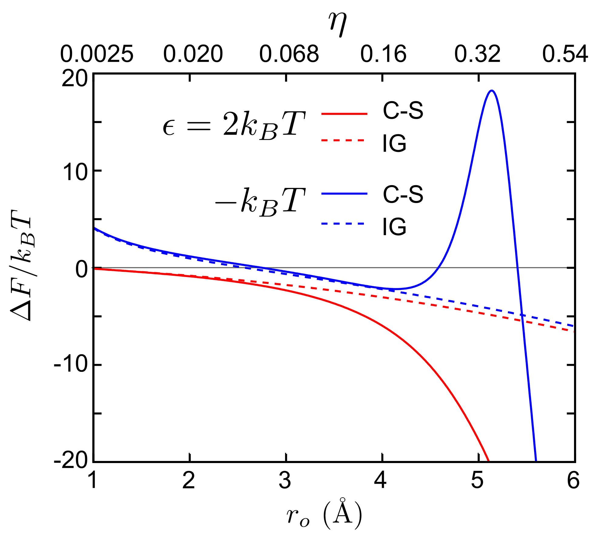
Figure 3: Total free energy change $\Delta F$ upon collapse in units of $k_{{\tiny B}}T$, as a function of osmolyte radius $r_{o}$. Values of packing fraction $\eta$ corresponding to the values of $r_{o}$ on the x-axis are shown above the plot. Curves are taken from equation (7) which combines surface area and volume terms. Here the polymer length $N_{p}=70$, the osmolyte concentration $\rho=1$M, and $r_{a}=6$Å. Red curves show $\Delta F$ upon collapse for a repulsive osmolyte with interaction energy $+2k_{{\tiny B}}T$, i.e. a crowding particle. Blue curves show $\Delta F$ upon collapse for an attractive osmolyte with interaction energy $-k_{{\tiny B}}T$, i.e. a weak denaturant. Plotted are both the model with ideal gas (IG, dashed) and Carnahan-Starling (C-S, solid) pressure and chemical potential.

3 The Density Functional Theory Formulation

We now consider a density functional formulation of the problem of transfer free energy. In what follows, we will assume that the intra-protein energy of a given configuration of a protein is in principle known and the net interaction between any given site on the protein and either the osmolyte or water is in principle known. We then wish to calculate $\Delta F$, the free energy of transferring the protein from water to an osmolyte solution, or, equivalently, of transferring the osmolytes from an aqueous solution to one containing the protein (see 1). In short, we wish to consider the effect that the presence of osmolytes has on the free energy of the protein.

The uniqueness of the Kohn-Sham density functional may be extended to finite temperatures, so that the free energy of the protein-solvent system is uniquely expressed as a functional of the single particle density $\phi(\bm{r})$ ⁸⁰. We thus seek an expression for the free energy of the osmolytes and water in an arbitrary external potential. For our purposes in obtaining a transfer free energy, we will treat a given protein configuration, with atom positions $\{\bm{R}_{i}\}$, as the source of the external potential. We write the free energy in the standard way ⁵⁴:

$$F(\{\bm{R}_{i}\})= \int d^{3}r\>k_{B}T(-S_{o}(\phi_{o}(\bm{r}))-S_{w}(\phi_{w}(\bm{r})))+\mathcal{V}_{o}(\bm{r})\phi_{o}(\bm{r})+\mathcal{V}_{w}(\bm{r})\phi_{w}(\bm{r})$$

$$+\Phi_{o}[\phi_{o}]+\Phi_{w}[\phi_{w}]+\Phi_{ow}[\phi_{o},\phi_{w}]$$ (9)

Here $\phi_{j}$ is the density function for the osmolytes $(o)$ or water $(w)$, and $\mathcal{V}_{j}$ the external potential on the respective species. The entropy density for each species can be written as

$$S_{o}(\bm{r})+S_{w}(\bm{r})=-\phi_{o}(\bm{r})\log\left[\lambda_{o}^{3}\phi_{o}(\bm{r})\right]-\phi_{w}(\bm{r})\log\left[\lambda_{w}^{3}\phi_{w}(\bm{r})\right]$$ (10)

where $\lambda_{o}$ and $\lambda_{w}$ are constants with units of length, analogous to thermal wavelengths. The terms $\Phi_{o}$, $\Phi_{w}$, and $\Phi_{ow}$ are the multi-particle correlation contributions to the free energy for the respective species. For example, the two particle correlation part of $\Phi_{o}$ would have the form

$$\Phi_{o}^{(2)}[\phi_{o}]=\int\int d^{3}r_{1}d^{3}r_{2}\>\phi_{o}(\bm{r}_{1})\phi_{o}(\bm{r}_{2})U_{oo}(\bm{r}_{1}-\bm{r}_{2})g(\bm{r}_{1},\bm{r}_{2}|\mathcal{V})$$ (11)

where $U_{oo}$ is the interaction potential between two osmolytes and $g$ the two-particle correlation function. The full multi-particle function is not known exactly, and so, as in electronic DFT, while equation (9) is exact in principle, approximations must be made to use it in practice  ⁸¹.

We now make two key assumptions. The first is that the water and osmolyte densities are completely correlated, such that all vacua are occupied by either water or osmolyte. Thus $N_{w}v_{w}+N_{o}v_{o}=V$, where $v_{i}$ is the volume of an individual water or osmolyte molecule, and $V$ the total volume. Dividing this by $Vv_{w}$ and allowing the local density of a given species to vary gives

$$\phi_{w}(\bm{r})+f\phi_{o}(\bm{r})=\rho_{w}$$ (12)

where $f=v_{o}/v_{w}$ and $\rho_{w}=1/v_{w}$ (the factor of $f$ allows for the osmolyte molecule to be a different size than the water molecule). Equation (12) is not valid in the interior of the protein, so we split our system up into two regions: a hard wall region $V_{hw}$ in which $\phi_{w}=\phi_{o}=0$, and the rest of the system, which has a volume $V$ identical to the volume of the osmolyte-water bath prior to the insertion of the protein, and in which Equation (12) is valid. We further take $V_{hw}$ to be same as the change in volume of the aqueous system the protein was removed from in the transfer process (see 1), so that the total system of water, protein, and osmolyte-water solution does not change volume during the transfer process.

With the approximation of equation (12) we can write

$$\mathcal{V}_{o}(\bm{r})\phi_{o}(\bm{r})+\mathcal{V}_{w}(\bm{r})\phi_{w}(\bm{r})= \Delta\mathcal{V}(\bm{r})\phi_{o}(\bm{r})+\mathcal{V}_{w}(\bm{r})\rho_{w}$$ (13)

$$\Phi_{o}[\phi_{o}]+\Phi_{w}[\phi_{w}]+\Phi_{ow}[\phi_{o},\phi_{w}]= \Phi_{t}[\phi_{o}]$$ (14)

where $\Delta\mathcal{V}(\bm{r})=\mathcal{V}_{o}(\bm{r})-f\mathcal{V}_{w}(\bm{r})$.

The second approximation in our treatment is that the osmolyte number density is much less than that of water. Using this approximation along with the one given in Equation (12), the entropy in Equation (10) becomes

$$-S_{o}(\bm{r})-S_{w}(\bm{r})= \phi_{o}(\bm{r})\log\left[\lambda_{o}^{3}\phi_{o}(\bm{r})\right]+(\rho_{w}-f\phi_{o}(\bm{r}))\log\left[\lambda_{w}^{3}(\rho_{w}-f\phi_{o}(\bm{r}))\right]$$ (15)

$$\approx \phi_{o}(\bm{r})\log\left[\lambda_{o}^{3}\phi_{o}(\bm{r})\right]-f\phi_{o}(\bm{r})+\rho_{w}\log\left[\lambda_{w}^{3}\rho_{w}\right]-f\phi_{o}(\bm{r})\log\left[\lambda_{w}^{3}\rho_{w}\right]$$

In this way we express each part of equation (9) in terms of osmolyte density and constant terms. The free energy functional may then be written as

$$F= \int d^{3}r\>k_{B}T(\phi_{o}(\bm{r})\log\left[\lambda_{o}\phi_{o}(\bm{r})\right]-(\gamma+1)\phi_{o}(\bm{r}))+\Delta\mathcal{V}(\bm{r})\phi_{o}(\bm{r})$$

$$+V\rho_{w}\log\lambda_{w}^{3}\rho_{w}+\mathcal{U}\rho_{w}+\Phi_{t}[\phi_{o}]$$ (16)

where $\mathcal{U}\equiv\int d^{3}r\mathcal{V}(\bm{r})$, and $\gamma+1\equiv f(1+\log(\lambda_{w}^{3}\rho_{w}))$. Since $V$ is the volume of the system, the term $V\rho_{w}$ is equal to $V/v_{w}=N_{w}^{\prime}$, the total number of water molecules in a system of pure water of volume $V$.

Thus, dropping the subscripts, letting $\mathcal{V}\equiv\Delta\mathcal{V}$, and ignoring any position independent terms, we can write the free energy as

$$F= \int d^{3}r\>k_{B}T\left(\phi(\bm{r})\log\lambda^{3}\phi(\bm{r})-\phi(\bm{r})\right)+k_{B}T\gamma\phi(\bm{r})+\mathcal{V}(\bm{r})\phi(\bm{r})$$

$$+\Phi[\phi]$$ (17)

where $\Phi[\phi]$ is the functional containing the multi-particle correlation part of the free energy, and $\lambda\equiv\lambda_{o}$ is a constant with units of length analogous to the thermal wavelength, whose value will be shown to be unimportant. For now we will formally manipulate $\Phi$ without making assumptions about its form. We can find the density that minimizes the free energy by use of the Euler-Lagrange equations, with the constraint that the osmolyte density when integrated over the total volume is the total number of osmolytes:

$$\int_{V}d^{3}r\>\phi(\bm{r})=N_{o}\>.$$ (18)

We thus write

$$\frac{\delta}{\delta\phi}\left[F-\mu_{o}\left(\int_{V}d^{3}r\>\phi(\bm{r})-N_{o}\right)\right] =0$$

$$\mbox{or}\;\;\;\;\;k_{B}T\log\lambda^{3}\phi(\bm{r})+\mathcal{V}(\bm{r})-k_{B}T\gamma+\frac{\delta\Phi}{\delta\phi}-\mu_{o} =0$$ (19)

where $\mu_{o}$ is the Lagrange multiplier corresponding to the constraint in equation (18). Physically, we can interpret equation (19) as a statement that $\frac{\delta F}{\delta\phi}$ is equal to the chemical potential $\mu_{o}$, and thus must be a constant value at all points in space. Solving this for the density field gives

$$\phi(\bm{r})=\mathrm{e}^{\gamma}\lambda^{-3}\mathrm{e}^{-\beta(\mathcal{V}(\bm{r})+\Phi^{\prime}-\mu_{o})}$$ (20)

where $\Phi^{\prime}\equiv\frac{\delta\Phi}{\delta\phi}$.

To obtain $\mu_{o}$ from equation (20), we use the constraint on the total number of particles in equation (18) which yields

$$\mathrm{e}^{\beta\mu_{o}}=\frac{\mathrm{e}^{\gamma}\lambda^{3}N_{o}}{\int_{V}d^{3}r\>\mathrm{e}^{-\beta(\mathcal{V}(\bm{r})+\Phi^{\prime})}}\>.$$ (21)

From here we can obtain the transfer free energy, which is given by the free energy of the osmolyte bath in the presence of the external protein potential, $\mathcal{V}(\bm{r})$, minus the free energy of the osmolyte bath without the protein potential $(\mathcal{V}(\bm{r})=0$). We thus have

$$\Delta F= \Delta\mu_{o}N_{o}$$

$$= -k_{B}TN_{o}\log\left(\frac{\mathrm{e}^{\gamma}\lambda^{-3}}{N_{o}}\int_{V}d^{3}r\>\mathrm{e}^{-\beta(\mathcal{V}(\bm{r})+\Phi^{\prime}_{f}(\bm{r}))}\right)$$

$$+k_{B}TN_{o}\log\left(\frac{\mathrm{e}^{\gamma}\lambda^{-3}}{N_{o}}\int_{V}d^{3}r\>\mathrm{e}^{-\beta\Phi^{\prime}_{i}}\right)$$ (22)

where the volume $V$ integrated over is the volume outside of hard-wall volume of the protein, and is the same in the initial and final systems. The difference $\Delta F$ is independent of $\lambda$ and $\gamma$.

The bath in the initial state is homogeneous and isotropic, so $\Phi^{\prime}_{i}$ in equation (22) is independent of position. Thus it may be factored out of the integral,

$$\int_{V}d^{3}r\>\mathrm{e}^{-\beta\Phi^{\prime}_{i}}=V\mathrm{e}^{-\beta\Phi^{\prime}_{i}}$$

so that

$$\Delta F=-k_{B}TN_{o}\log\left(\frac{1}{V}\int_{V}d^{3}r\>\mathrm{e}^{-\beta(\mathcal{V}(\bm{r})+\Delta\Phi^{\prime})}\right)$$ (23)

where $\Delta\Phi^{\prime}=\Phi^{\prime}_{f}(\bm{r})-\Phi^{\prime}_{i}$. The expression in equation (23) consists of the logarithm of the integral of a Boltzmann weight for the effective potential $\mathcal{V}(\bm{r})+\Delta\Phi^{\prime}(\bm{r})$. Here $\mathcal{V}(\bm{r})$ and $\Delta\Phi^{\prime}(\bm{r})$ enter on equal footing. Recall that $\mathcal{V}$ is the protein-osmolyte potential, treating the protein as an external source. $\Phi^{\prime}$ is the functional derivative of the multi-particle part of the free energy. If we use the two-particle osmolyte contribution from equation (11), we obtain

$$\Delta\Phi_{o}^{(2)\prime}=\left.\frac{\delta\Phi_{o}^{(2)}}{\delta\phi_{o}(\bm{r})}\right|_{\mathcal{V}}-\left.\frac{\delta\Phi_{o}^{(2)}}{\delta\phi_{o}(\bm{r})}\right|_{\mathcal{V}=0}=\int d^{3}r^{\prime}\>\left[\phi_{of}(\bm{r}^{\prime})g(\bm{r},\bm{r}^{\prime}|\mathcal{V})-\phi_{oi}(\bm{r}^{\prime})g(\bm{r},\bm{r}^{\prime}|\mathcal{V}=0)\right]U_{oo}(\bm{r},\bm{r}^{\prime})\>,$$ (24)

which gives the difference of two terms in the presence and absence of the external protein potential, where each term corresponds to the equilibrium-averaged interaction energy between osmolytes, up to pair correlations. Thus the term $\Delta\Phi^{\prime}$ in Equation (23) can be interpreted as the change in energy due to redistribution of the environment in response to the change in external potential.

We can recast equation (23) into a form that will be somewhat more useful later:

$$\Delta F=-k_{B}TN_{o}\log\left(1+\frac{1}{V}\int_{V}d^{3}r\>[\mathrm{e}^{-\beta(\mathcal{V}(\bm{r})+\Delta\Phi^{\prime})}-1]\right)$$ (25)

which has the advantage that when $\mathcal{V}$ and $\Delta\Phi^{\prime}$ are both zero, the integrand is also zero, and thus the integral can be taken over all space.

In equation (25) we can take the limit $V\rightarrow\infty$, with $N_{o}/V=\rho$ fixed. Then, assuming that the region over which the integrand in equation (25) is non-zero is finite, we can expand the logarithm to first order to obtain

$$\Delta F=-k_{B}TN_{o}\frac{1}{V}\int d^{3}r\>\left(\mathrm{e}^{-\beta(\mathcal{V}(\bm{r})+\Delta\Phi^{\prime})}-1\right)$$ (26)

which has the form

$$\Delta F=p_{id}\Delta V_{\mathrm{eff}}$$

where $p_{id}=N_{o}k_{{\tiny B}}T/V$ is the ideal gas osmotic pressure, and $V_{\mathrm{eff}}=\int d^{3}r\>\left[1-\mathrm{e}^{-\beta(\mathcal{V}(\bm{r})+\Delta\Phi^{\prime})}\right]$ is an effective change in volume. In the dilute limit, the osmotic pressure $p=p_{id}$; then $V_{\mathrm{eff}}$ may be interpreted as the change in volume available to the osmolytes.

We now need to address $\Delta\Phi^{\prime}$ to progress further. The obvious first approximation is to set $\Delta\Phi^{\prime}=0$; we will see below that this approximation can in fact go quite a long way, depending on the solvent. This is consistent with the observations in 3 where the ideal gas approximation, which neglects osmolyte-osmolyte correlations, holds for typical molecular radii at 1M concentration. It is worth noting that this is not ignoring the osmolyte-osmolyte, osmolyte-water, and water-water correlations completely; it is merely assuming that they are the same in the initial and final baths. Making this approximation, we have

$$\Delta F=-k_{B}TN_{o}\log\left(1+\frac{1}{V}\int_{V}d^{3}r\>[\mathrm{e}^{-\beta\mathcal{V}(\bm{r})}-1]\right)$$ (27)

Equation (27) represents an approximation to the transfer free energy that, while severe, nonetheless takes into account both the change in energy and change in entropy of the osmolyte bath.

3.1 Validation tests in model solvents

As a test of the density functional theory, we have used equation (27) to calculate the transfer free energy of several small molecules into model osmolytes. To simplify the simulations, we looked at transfer from vacuum to a van der Waals gas of osmolytes, which were taken to be single atoms interacting through a VDW potential. The density of the osmolytes was set to 1M. The molecules we transferred were the side chains of alanine and valine, with C-$\beta$ capped with a hydrogen to replace the backbone (ie, the molecules were methane and propane). The coordinates were taken from an existing protein structure file, and the angle and bond parameters were generated with the GROMACS utility pdb2gmx. The charges were set to zero for all atoms, and the interaction was purely van der Waals. We list the VDW parameters in 1. 4 shows the interaction potential for the two different osmolytes we used. The transfer energies were calculated both with equation (27) and by simulating the transfer in GROMACS and using Thermodynamic Integration (TI) ^{82, 83, 84}. The results are summarized in 2, and show excellent agreement between TI and DFT. This is notable since the result was obtained neglecting the inter-particle correlations, and at 1M the pressure of the osmolytes was $\approx 1.5$ that of the ideal gas pressure, which indicates that the osmolyte-osmolyte interactions were significant.

Atom	$\sigma$ (Å)	$\epsilon$ (kJ/mol)
Ala C-$\beta$	0.36705	0.33472
Ala H	0.23520	0.092048
Val C-$\beta$	0.40536	0.08368
Val C-$\gamma$	0.36705	0.33472
Val H	0.23520	0.092048
Osm1	0.40536	0.08368
Osm2	0.36705	0.33472

Table 1: van der Waals parameters for the atoms used in the simulation test of the DFT, as taken from the CHARMM parameter set. Osm2 is a relatively attractive spherical osmolyte, while the potential of Osm1 is dominated by steric repulsion. The interaction is parameterized as $V(r)=4\epsilon\left[\left(\sigma/r\right)^{12}-\left(\sigma/r\right)^{6}\right]$.

Molecule/Osmolyte	DFT $\Delta G$ (kJ/mol)	TI $\Delta G$ (kJ/mol)
Ala/Osm1	$0.188\pm 0.002$	$0.187\pm 0.002$
Val/Osm1	$0.255\pm 0.004$	$0.261\pm 0.004$
Ala/Osm2	$0.055\pm 0.002$	$0.059\pm 0.003$
Val/Osm2	$-0.018\pm 0.004$	$-0.011\pm 0.004$

Table 2: Comparison of test cases between density functional theory (DFT) and thermodynamic integration (TI)

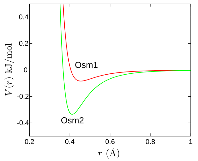
Figure 4: Comparison of osmolyte potential functions for the test cases parameterized in 1. Osm2 is significantly more attractive than Osm1, which is reflected in the transfer free energies in 2

3.2 Connecting DFT to previous surface/volume models

We now take a simplified model of a protein potential to compare with the results obtained previously in Section 2 for the solvent contribution to the change in free energy upon protein collapse. In this model we will consider the protein to have an excluded volume of $V_{prot}$; that is, within that volume the potential is infinite. From the discussion in sections 2.1-3 concerning excluded volume, we saw that the changes in volume treated there are volumes from which osmolytes are excluded. We also consider the protein to have a surface region of thickness $t$ that exerts a potential on the osmolytes of depth $\epsilon$; this region is sufficiently thin that we can approximate its volume as $V_{surface}\approx tA$. If we use this model in the expression for the free energy in the limit of large system size (equation (27) ) then we obtain a free energy upon transfer of

$$\Delta F=\rho k_{{\tiny B}}T\left(V_{prot}+(1-\mathrm{e}^{-\beta\epsilon})tA\right)\>.$$ (28)

The DFT transfer free energy with this simplified model provides a natural split between the volume contribution $p_{id}V_{prot}$ and the surface area contribution $p_{id}(1-\mathrm{e}^{-\beta\epsilon})tA$. Thus the DFT result, in the appropriate model, naturally generates the free energy contributions derived in section 2 from more bespoke considerations. Specifically, if we take the total volume of the protein upon insertion to be $V=V_{prot}+tA$, then equation (28) is identical to equation (8). The simplified DFT model here reduces to our earlier considerations and helps give a physical interpretation of the quantity $\rho_{Q}$ as it pertains to the protein surface.

We can also see that, in order to obtain an SASA approximation in which $\Delta F$ is independent of temperature, one would have to assume that the osmolyte-protein binding energy $\epsilon\ll k_{B}T$, and that volume terms were either negligible compared to surface terms, or they were proportional to them. We find below that $\epsilon\approx k_{{\tiny B}}T$ in order to obtain empirically-derived transfer free energies to TMAO, which does not satisfy the above inequality. As well, we can use the tube model from Section 2 for protein volume and surface area to estimate the relative contributions of volume and area: for an osmolyte of radius $r_{o}=2.5$ Å  and a protein with $N_{p}=70$, $V/tA=0.62$ in the unfolded state, and $V/tA=0.77$ in the folded state. The volume here is by no means negligible.

We thus expect on general grounds that the transfer free energy will be dependent on temperature. One way of looking at the simplified limit for the transfer free energy in equation (28) is as a derivation of a new phenomenological form for the transfer energy, containing both temperature and volume dependence:

$$\Delta F=\gamma_{1}k_{{\tiny B}}T(V_{solute})+\gamma_{2}k_{{\tiny B}}T(\mbox{ASA})\mathrm{e}^{-\beta\epsilon}\>,$$ (29)

where one can now fit the parameters $\gamma_{1}$, $\gamma_{2}$, and $\epsilon$, to empirical data.

4 Empirically Deriving DFT Transfer Free Energy Parameters

The potential $\mathcal{V}(\bm{r})$ in equation (27) is an effective potential given by $\mathcal{V}_{o}(\bm{r})-f\mathcal{V}_{w}(\bm{r})$. Obtaining $f$ and $\mathcal{V}_{w}$ may be nontrivial to obtain ab initio, so we examine some model systems, and compare with empirical methods. To begin with, we will assume that the potential takes the form of a sum of terms from each particle in the protein, where a particle may be an atom in an all-atom model, or a bead modeling an amino acid in a coarse-grained approach:

$$\mathcal{V}(\bm{r})=\sum_{i=1}^{N_{p}}v^{\mathrm{eff}}_{i}(\bm{r}-\bm{R}_{i})\>.$$

Here $N_{p}$ is the number of particles in the protein, and $\bm{R}_{i}$ the position of the $i$th particle.

We consider a model consisting of backbone $C_{\alpha}$ atoms and coarse-grained side-chain beads, which then form the particles for our potential. We make the assumption that the protein-osmolyte potentials have a 6-12 form:

$$v_{i}(r)=4\epsilon_{i}\left[\left(\frac{\sigma_{i}}{r}\right)^{12}-\left(\frac{\sigma_{i}}{r}\right)^{6}\right]\>,$$

and we wish to determine the potential parameters $\sigma_{i}$, $\epsilon_{i}$ for each amino acid that reproduce the transfer energies found experimentally when DFT is applied using the above potential. As a starting point, we examine those used by Auton and Bolen ⁸⁵.

Two constraint equations are required for each amino acid. For the first equation, we note that the beads representing the various amino acid side chains have residue radii $r_{oi}$ that may be obtained from measured partial molar volumes ⁸⁶. We can then apply a constraint to the above 6-12 parameters $\sigma_{i}$, $\epsilon_{i}$ by requiring that at a distance $r_{oi}$ from the residue centre,

$$v_{i}(r_{oi})=0.6\;\>\mbox{kcal}\cdot\mbox{mol}^{-1}\>.$$ (30)

To obtain the remaining equation determining the parameters $\sigma_{i}$, $\epsilon_{i}$, we require that the DFT transfer free energy, as computed by the dilute limit of equation (27) for the single particle representing an amino acid side chain, should be equal to the experimental value as given in reference ⁸⁵, specifically for transfer into a solution of 1M TMAO. This involves computing the integral over the osmolyte-accessible volume in the expression

$$\rho k_{{\tiny B}}T\int d^{3}r\left(1-\mathrm{e}^{-\beta v_{i}(r)}\right)$$ (31)

and setting the result to the empirical value of $\delta g_{i}$ for each amino acid.

The sum of the transfer free energies of each amino acid in a Gly-X-Gly tripeptide is often used to approximate the conformationally-averaged transfer free energy for a protein.⁸⁵ Here we consider the tripeptide transfer free energies. The integral in expression (31) then involves integration over a solid angle $\Omega_{i}$ determined by the fraction of solid angle available to the side chain in the tripeptide vs. that for the isolated residue, i.e.

$$\Omega_{i}=\frac{A^{i}_{tri}}{A^{i}_{iso}}4\pi$$

The potential $v_{i}$ is then fully determined from equation (30) along with

$$\Omega_{i}\rho k_{{\tiny B}}T\int_{0}^{\infty}dr\>r^{2}\left(1-\mathrm{e}^{-\beta v_{i}(r)}\right)=\delta g_{i}\>.$$ (32)

We can now construct potentials for each amino acid transfer free energy given in reference ¹⁸. The parameters derived from doing so are listed in 3. The backbone-osmolyte interaction was parameterized as $v_{BB}(r)=C/r^{12}$, as this better represented it’s strongly repulsive character. The value of $C$ obtained by fitting to $\delta g_{BB}$ was $C=7.510\times 10^{7}$ kcal$\cdot$Ź².

In this context, the DFT formulation provides a way of using the information from tri-peptide experiments in a way that captures both energetic and entropic effects. The parameters just obtained can be used to determine the change in the transfer free energies for isolated residues as temperature changes. The experimental transfer free energies $\delta g_{i}$ are predicted to increase as temperature increases, with the new values at $T=310$K given in 3. Increasing temperature by $0.03k_{{\tiny B}}T$ increases the transfer free energy by $\approx 0.6k_{{\tiny B}}T$ for a 100 residue protein. This change is not large, but the relative temperature change is also small. The transfer entropy is significant: $d(\delta g)/dT\approx 20k_{{\tiny B}}$.

Table 3: Parameter values yielding transfer free energies $\delta g$ to 1M TMAO for amino acid side chains and backbone at 300K, and the predicted $\delta g$ at 310K .

Type	$r_{o}$ (Å)	$\delta g$ (cal/mol)	$\sigma$ (Å)	$\epsilon$ (kcal/mol)	$\delta g(T=310K)$ (cal/mol)
Ala	2.52	-14.64	3.517	0.6286	-12.65
Arg	3.28	-109.3	4.088	1.022	-104.0
Asn	2.74	55.69	4.564	0.0483	58.06
Asp	2.79	-66.67	3.627	1.055	-63.31
Gln	3.01	41.41	4.397	0.1710	44.57
Glu	2.96	-83.25	3.799	0.9973	-78.88
His	3.04	42.07	4.428	0.1707	45.28
Ile	3.09	-25.43	4.084	0.5692	-21.59
Leu	3.09	11.6	4.246	0.3405	15.15
Lys	3.18	-110.23	3.968	1.126	-104.7
Met	3.09	-7.65	4.154	0.4538	-3.791
Phe	3.18	-9.32	4.237	0.4587	-5.397
Pro	2.78	-137.7	3.457	1.987	-133.5
Ser	2.59	-39.04	3.4905	0.8849	-36.45
Thr	2.81	3.75	3.9312	0.3889	6.41
Trp	3.39	-152.9	4.157	1.150	-146.5
Tyr	3.23	-114.3	4.020	1.103	-109.2
Val	2.93	-1.02	4.021	0.4238	1.78
BB	2.25	90.0	-	-	92.7

5 Using DFT for Implicit Solvent Models

The DFT methodology has been applied to the problem of solvation to calculate fluid correlation functions, solvation free energies, and reorganization energy in charge transfer ^{66, 67}. The use of time-dependent density functional theory has been well-established to understand solvation dynamics in single-component solvents ⁸⁷ as well as selective solvation in binary mixtures ^{88, 89}. The methodology has also been applied to the connect static and dynamic approaches to the glass transition by Kirkpatrick and Wolynes ⁴⁵. The DFT methodology as described above may also be be applied to the problem of finding the effective forces for molecular dynamics simulation in an implicit solvent, which we briefly describe here.

We again write the external potential due to solute-solvent interactions as

$$\mathcal{V}(\bm{r})=\sum_{j}v_{j}(|\bm{R}_{j}-\bm{r}|)$$

we can write the force on the $i$th particle from the transfer free energy in equation (26) (neglecting solvent inter-particle correlations) as

$$\mathbf{F}_{i} =\nabla_{R_{i}}\left[k_{B}T\rho\int d^{3}r\>\left(1-\mathrm{e}^{-\beta\sum_{j}v_{j}(|\bm{R}_{j}-\bm{r}|)}\right)\right]$$

$$=k_{B}T\rho\beta\int d^{3}r\>\mathrm{e}^{-\beta\sum_{j}v_{j}(|\bm{R}_{j}-\bm{r}|)}\nabla_{R_{i}}v_{i}(|\bm{R}_{i}-\bm{r}|)$$

$$=\rho\int d^{3}r\>\mathrm{e}^{-\beta\sum_{j}v_{j}(|(\bm{R}_{j}-\bm{R}_{i})-\bm{r}|)}\nabla v_{i}(r)$$ (33)

We immediate see that the integrand is non-zero only when $\nabla v_{i}(r)$ is non-zero, so that if there is an effective cutoff $r_{c}$ such that $v_{i}(r)\approx 0$ for $r>r_{c}$, then the integral in equation (33) only needs to be taken in the region $r<r_{c}$. This is a generalization of the result obtained by Götzelmann et al⁹⁰, who have shown that for a hard sphere potential, only the solvent density at the surface of the spheres was relevant to the calculation of depletion forces. Here we extend this analysis to arbitrary potentials.

Consider a particle with a spherically symmetric $v_{i}(r)$, as assumed above. The net force on this particle when isolated is zero. When a second particle exerting potential $v_{j}(r)$ on the osmolytes is brought near, the net force on the first due to the solvent is a result of the now asymmetric solvent density. We note here we are treating the indirect force rather than the direct force between the particles, which can be calculated by direct application of the interparticle potential. The region of asymmetric solvent density constitutes a restricted volume to be integrated over in equation (33), as only the region of overlap between the two spheres defined by the cutoff in potential around $\bm{R}_{i}$ and $\bm{R}_{j}$ contributes to the net force (see e.g. 5b below). In addition, the solvent field in this overlap region will maintain cylindrical symmetry about the axis joining the two particles, which means that the force will be along this axis as well. This suggests that the force on particle $i$ can be written as

$$\bm{F}_{i}=\sum_{|\bm{R}_{ij}|<2r_{c}}F_{ij}(|\bm{R}_{ij}|)\hat{\bm{R}}_{ij}\>.$$

Here $\hat{\bm{R}}_{ij}$ is the unit vector from particle $j$ to particle $i$, and $F_{ij}$ is a scalar function of the interparticle distance $|\bm{R}_{ij}|\equiv|\bm{R}_{i}-\bm{R}_{j}|$, which is determined by the overlap integral in equation (33), and which could in principle be pre-computed and tabulated to speed up execution.

5.1 Depletion and impeded-solvation interactions in an implicit solvent model

We can use equation (33) to investigate the forces due to solvent on colloidal particles. In what follows, we imagine the “solvent” to be simplified osmolytes within an implicit solvent bath. This subject has been well-studied (see e.g. refs. ^{91, 92, 93, 94, 95} ); our goal here is simply to show that the DFT transfer free energy provides a natural way of calculating depletion forces as well as transfer energies, and that even the approximated form in equation (33) yields non-trivial results for the depletion force.

We investigate a model consisting of two spheres that interact only by a hard wall potential of radius $r_{s}$. Each sphere also interacts with a bath of osmolytes through a 6-12 (van der Waals) potential: $V(r)=4\epsilon\left(\left(\sigma/r\right)^{12}-\left(\sigma/r\right)^{6}\right)$, with $\sigma=r_{s}+r_{o}$. With this model we examine the force as a function of the sphere separation $d$. Any force between the spheres is entirely due to osmolyte-mediated effects.

When the solute particles are far apart, they dress themselves with osmolyte solvation shells because of the attractive solute-osmolyte potential. As we imagine moving the two solute particles closer together, eventually the repulsive region of one solute particle overlaps with the attractive region of the other solute particle, and vice versa. This situation is unfavorable for the solute particles, and the energy may be lowered by moving them further apart; hence there is a repulsive force at these distances (see 5). As the solute particles continue to approach each other, the above repulsive region encroaches on the regions of space where the van der Waals potential is deeper. A larger amount of potentially favorable binding energy is removed per distance travelled, and the repulsive force due to “impeded-solvation” increases. The repulsive force is maximal when the solute separation $d$ is roughly $2\sigma$. For separations $d<2\sigma$, the repulsive regions of the two solute spheres begin to overlap. This reduces the volume excluded, or more precisely repulsive to, osmolytes. This reduced excluded volume results in an attractive force which is the traditional depletion force. Eventually the depletion force becomes stronger than the above impeded-solvation force, and the net force becomes attractive. We note that such effects would not be present in standard GB/SA models of implicit solvation.

In general, direct inter-particle interactions must be superimposed on the above scenario. Which force dominates at a given separation will then depend on the values for $r_{s}$, $r_{o}$, and $\epsilon$, along with the strength of the direct interaction. The above-described repulsive effect has been observed before in hard-sphere solutes using the Derjaguin approximation to obtain an effective surface tension ⁹⁰. Here we see that the effect arises naturally from the presence of an attractive potential in the density functional theory.

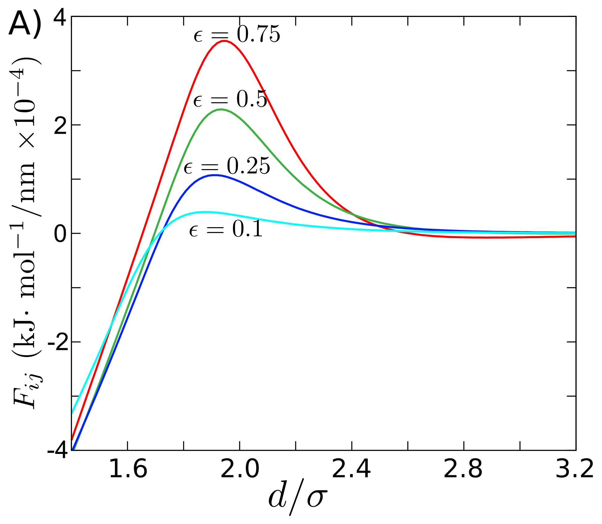
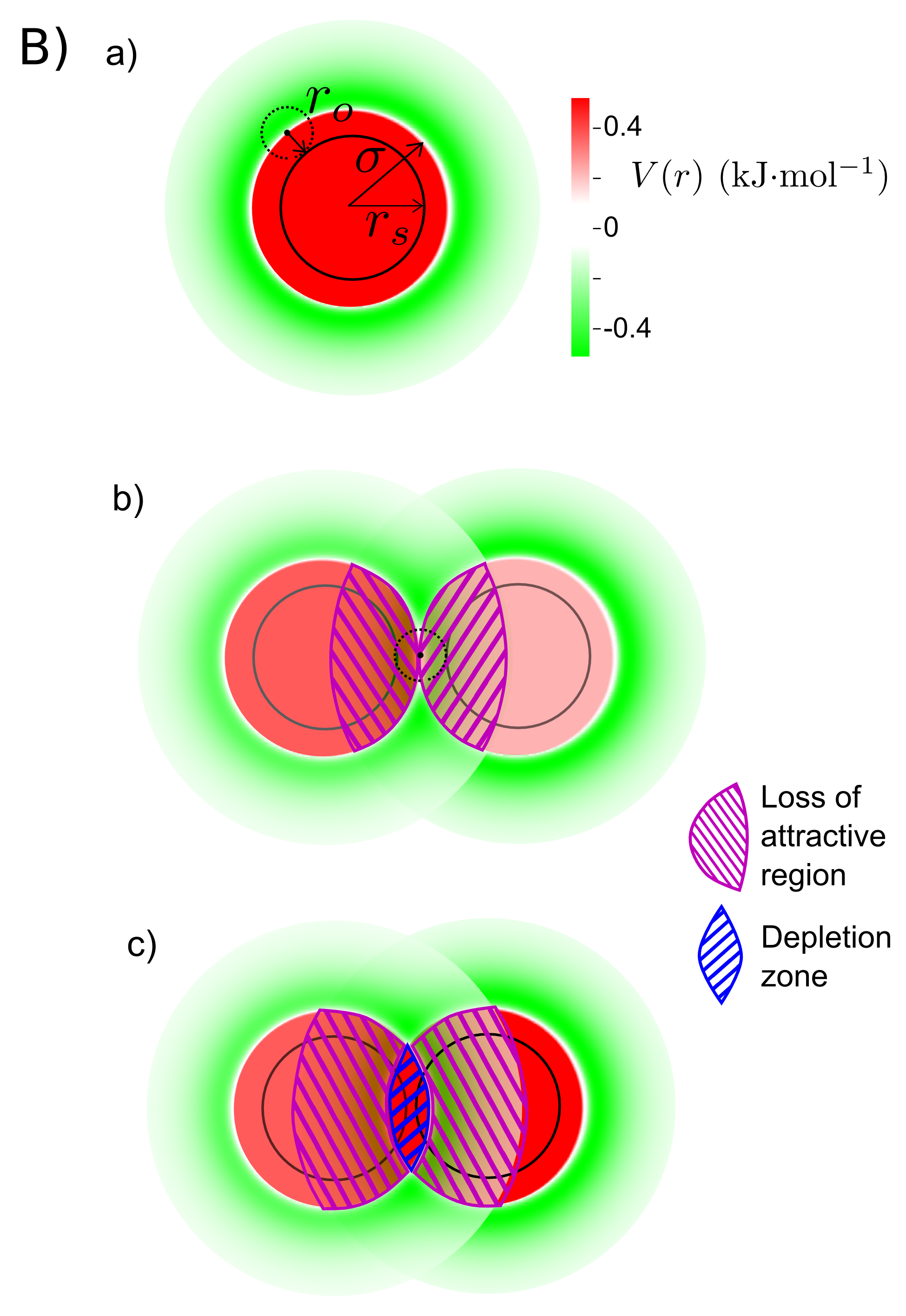
Figure 5: (A) Solvent-induced force on a pair of “hard-wall” spheres as a function of the separation distance, as obtained from equation (33). Spheres interact with osmolytes through a LJ potential (see text). The only parameters that determine the force are thus $\sigma$ and $\epsilon$, which appear in the LJ potential that enters into the DFT expression for the force. Each curve in the figure corresponds to a given well-depth $\epsilon$ in the sphere-osmolyte potential. The depletion force is dominant at small separation, but there is a region in which the spheres are mutually repulsive due to lost attraction or “impeded-solvation” to the solvent. (B) Schematic renderings of the solute spheres in (A) at several distances. a) The sphere-osmolyte interaction is through a LJ potential, which is negative beyond a distance $\sigma=r_{s}+r_{o}$ (shown as the green region), and positive and repulsive for $d<\sigma$ (red region). The direct sphere-sphere interaction is only through a hard-wall potential of radius $r_{s}$. The osmolytes have radius $r_{o}$. (b) Sphere configuration when distance $d=2\sigma$. An osmolyte can just fit between the spheres at this distance- the LJ potential is zero in this configuration if the osmolyte (dashed sphere) is centered directly between the solute particles. Such separations have positive force between the solutes in 5a, due to “impeded-solvation”: the repulsive interaction between one sphere-osmolyte pair removes some of the attractive region from the other sphere-osmolyte pair (region shown in magenta). At the separation shown in (c), the solvent-induced force between the spheres is now attractive; the volume of the removed attractive region now varies weakly with separation, and bringing the spheres closer together gains free energy by removing the depletion zone highlighted in blue.

6 Conclusions

In this paper we have explored the application of the density functional framework to protein transfer free energies. We have focused primarily on conceptual questions, such as the role of solvent excluded volume, the temperature dependence of transfer free energies, and how the density functional theory (DFT) would reduce to a Volume + SASA model of transfer free energy.

We compared the DFT results with those from a simplified model that treated the protein as a tube with a given volume and surface area, on which osmolytes could condense. The DFT contains contributions from both enthalpy and entropy, so it allows for the calculation of the temperature-dependence of the transfer free energy.

A further development of the theory presented here which accounts for interparticle correlations while maintaining computational efficiency is an important topic for future research. As well, the calculation of transfer free energies was implemented here for a model system with simplified potentials that were parameterized to experimental values. One could extend this by implementing the theory using more realistic potential models, and all-atom representations of a protein or peptide. The various approximations involved in these potentials and models could then be tested and the limits of their validity determined through comparisons with experiment and simulation. The DFT framework may also provide a method to obtain computationally efficient but still accurate implicit solvent models for molecular dynamics simulation, a subject of immense practical importance. In general, the framework of density functional theory can provide a powerful tool to explore aspects of solvation in the context of protein folding, and can do so in a systematic way.

7 Acknowledgements

S.S.P acknowldeges funding support from PrioNet Canada, NSERC, and computational support from the WestGrid high-performance computing consortium. E.A.M. has been supported by the NSERC PGSD program for the early part of this work. Lastly, S.S.P. would like to express his gratitude to Peter G. Wolynes, for providing some of the most enlightening and enjoyable years of his research career- if only I knew then what I know now!

References

- Persson and Halle 2008 Persson, E.; Halle, B. Cell Water Dynamics on Multiple Time Scales. Proc. Natl. Acad. Sci. U. S. A. 2008, 105, 6266–6271
- Yancey et al. 1982 Yancey, P.; Clark, M.; Hand, S.; Bowlus, R.; Somero, G. Living with Water Stress: Evolution of Osmolyte Systems. Science 1982, 217, 1214–1222
- Ellis and Minton 2006 Ellis, R. J.; Minton, A. P. Protein Aggregation in Crowded Environments. Biol. Chem. 2006, 387, 485–497
- Zhou et al. 2008 Zhou, H.-X.; Rivas, G.; Minton, A. P. Macromolecular Crowding and Confinement: Biochemical, Biophysical, and Potential Physiological Consequences. Annu. Rev. Biophys. 2008, 37, 375–397
- Minton 2001 Minton, A. P. The Influence of Macromolecular Crowding and Macromolecular Confinement on Biochemical Reactions in Physiological Media. J. Biol. Chem. 2001, 276, 10577–10580
- Ellgaard and Helenius 2003 Ellgaard, L.; Helenius, A. Quality Control in the Endoplasmic Reticulum. Nat. Rev. Mol. Cell. Biol. 2003, 4, 181–191
- Canchi et al. 2010 Canchi, D. R.; Paschek, D.; García, A. E. Equilibrium Study of Protein Denaturation by Urea. J. Am. Chem. Soc. 2010, 132, 2338–2344
- Linhananta et al. 2011 Linhananta, A.; Hadizadeh, S.; Plotkin, S. S. An Effective Solvent Theory Connecting the Underlying Mechanisms of Osmolytes and Denaturants for Protein Stability. Biophys. J. 2011, 100, 459–468
- Friedel et al. 2003 Friedel, M.; Sheeler, D. J.; Shea, J.-E. Effects of Confinement and Crowding on the Thermodynamics and Kinetics of Folding of a Minimalist Beta-barrel Protein. J. Chem. Phys. 2003, 118, 8106–8113
- Cheung et al. 2005 Cheung, M. S.; Klimov, D.; Thirumalai, D. Molecular Crowding Enhances Native State Stability and Refolding Rates of Globular Proteins. Proc. Natl. Acad. Sci. U. S. A. 2005, 102, 4753 – 4758
- Ionescu-Tirgoviste and Despa 2011 Ionescu-Tirgoviste, C.; Despa, F. Biophysical Alteration of the Secretory Track in -cells due to Molecular Overcrowding: the Relevance for Diabetes. Integr. Biol. 2011, 3, 173–179
- Minton 2000 Minton, A. P. Implications of Macromolecular Crowding for Protein Assembly. Curr. Opin. Struct. Biol. 2000, 10, 34–39
- Wojciechowski and Cieplak 2008 Wojciechowski, M.; Cieplak, M. Effects of Confinement and Crowding on Folding of Model Proteins. BioSystems 2008, 94, 248–252
- Lee and Richards 1971 Lee, B.; Richards, F. The Interpretation of Protein Structures: Estimation of Static Accessibility. J. Mol. Biol. 1971, 55, 379–400
- Eisenberg and McLachlan 1986 Eisenberg, D.; McLachlan, A. D. Solvation Energy in Protein Folding and Binding. Nature 1986, 319, 199–203
- Tan et al. 2007 Tan, C.; Tan, Y.-H.; Luo, R. Implicit Nonpolar Solvent Models. J. Phys. Chem. B 2007, 111, 12263–12274
- O’Brien et al. 2008 O’Brien, E. P.; Ziv, G.; Haran, G.; Brooks, B. R.; Thirumalai, D. Effects of denaturants and osmolytes on proteins are accurately predicted by the molecular transfer model. Proc. Natl. Acad. Sci. U. S. A. 2008, 105, 13403–13408
- Auton and Bolen 2004 Auton, M.; Bolen, D. W. Additive Transfer Free Energies of the Peptide Backbone Unit That Are Independent of the Model Compound and the Choice of Concentration Scale†. Biochemistry 2004, 43, 1329–1342
- Soda 1993 Soda, K. Solvent exclusion effect predicted by the scaled particle theory as an important factor of the hydrophobic effect. J. Phys. Soc. Jpn. 1993, 62, 1782–1793
- Saunders et al. 2000 Saunders, A.; Davis-Searles, P. R.; Allen, D. L.; Pielak, G. J.; ; Erie, D. A. Osmolyte-induced changes in protein conformation equilibria. Biopolymers 2000, 53, 293–307
- Schellman 2003 Schellman, J. A. Protein Stability in Mixed Solvents: A Balance of Contact Interaction and Excluded Volume. Biophys. J. 2003, 85, 108–125
- Imai et al. 2007 Imai, T.; Harano, Y.; Kinoshita, M.; Kovalenko, A.; Hirata, F. Theoretical analysis on changes in thermodynamic quantities upon protein folding: Essential role of hydration. J. Chem. Phys. 2007, 126, 225102
- Wagoner and Baker 2006 Wagoner, J. A.; Baker, N. A. Assessing implicit models for nonpolar mean solvation forces: The importance of dispersion and volume terms. Proc. Natl. Acad. Sci. U. S. A. 2006, 103, 8331–8336
- Qiu et al. 1997 Qiu, D.; Shenkin, P. S.; Hollinger, F. P.; Still, W. C. The GB/SA Continuum Model for Solvation. A Fast Analytical Method for the Calculation of Approximate Born Radii. J. Phys. Chem. A 1997, 101, 3005–3014
- Roux and Simonson 1999 Roux, B.; Simonson, T. Implicit solvent models. Biophys. Chem. 1999, 78, 1 – 20
- Bashford and Case 2000 Bashford, D.; Case, D. A. Generalized Born models of macromolecular solvation effects. Annu. Rev. Phys. Chem. 2000, 51, 129–152
- Zhou and Berne 2002 Zhou, R.; Berne, B. J. Can a continuum solvent model reproduce the free energy landscape of a β-hairpin folding in water? Proc. Natl. Acad. Sci. U. S. A. 2002, 99, 12777–12782
- Gallicchio and Levy 2004 Gallicchio, E.; Levy, R. M. AGBNP: An analytic implicit solvent model suitable for molecular dynamics simulations and high-resolution modeling. J. Comput. Chem. 2004, 25, 479–499
- Labute 2008 Labute, P. The generalized Born/volume integral implicit solvent model: Estimation of the free energy of hydration using London dispersion instead of atomic surface area. J. Comput. Chem. 2008, 29, 1693–1698
- Chen et al. 2008 Chen, J.; III, C. L. B.; Khandogin, J. Recent advances in implicit solvent-based methods for biomolecular simulations. Curr. Opin. Struct. Biol. 2008, 18, 140 – 148
- Feig and III 2004 Feig, M.; III, C. L. B. Recent advances in the development and application of implicit solvent models in biomolecule simulations. Curr. Opin. Struct. Biol. 2004, 14, 217 – 224
- Chandler and Andersen 1972 Chandler, D.; Andersen, H. C. Optimized Cluster Expansions for Classical Fluids. II. Theory of Molecular Liquids. J. Chem. Phys. 1972, 57, 1930–1937
- Barker and Henderson 1976 Barker, J. A.; Henderson, D. What is "liquid"? Understanding the states of matter. Rev. Mod. Phys. 1976, 48, 587–671
- Hirata and Rossky 1981 Hirata, F.; Rossky, P. J. An extended RISM equation for molecular polar fluids. Chem. Phys. Lett. 1981, 83, 329–334
- Beglov and Roux 1997 Beglov, D.; Roux, B. An integral equation to describe the solvation of polar molecules in liquid water. J. Phys. Chem. B 1997, 101, 7821–7826
- Kovalenko et al. 1999 Kovalenko, A.; Ten-no, S.; Hirata, F. Solution of three-dimensional reference interaction site model and hypernetted chain equations for simple point charge water by modified method of direct inversion in iterative subspace. J. Comput. Chem. 1999, 20, 928–936
- Kovalenko and Hirata 1998 Kovalenko, A.; Hirata, F. Three-dimensional density profiles of water in contact with a solute of arbitrary shape: a RISM approach. Chem. Phys. Lett. 1998, 290, 237 – 244
- Mermin 1965 Mermin, N. D. Thermal properties of the inhomogeneous electron gas. Phys. Rev. 1965, 137, A1441
- Ebner et al. 1976 Ebner, C.; Saam, W. F.; Stroud, D. Density-functional theory of simple classical fluids. I. Surfaces. Phys. Rev. A 1976, 14, 2264–2273
- Evans 1979 Evans, R. The nature of the liquid-vapour interface and other topics in the statistical mechanics of non-uniform, classical fluids. Adv. Phys. 1979, 28, 143–200
- Chandler et al. 1986 Chandler, D.; McCoy, J. D.; Singer, S. J. Density functional theory of nonuniform polyatomic systems. I. General formulation. J. Chem. Phys. 1986, 85, 5971–5976
- Evans 1992 Evans, R. Density functionals in the theory of inhomogeneous fluids. In Fundamentals of inhomogeneous fluids; Henderson, D., Ed.; Dekker: New York, 1992
- Biben et al. 1998 Biben, T.; Hansen, J. P.; Rosenfeld, Y. Generic density functional for electric double layers in a molecular solvent. Phys. Rev. E 1998, 57, R3727–R3730
- Singh et al. 1985 Singh, Y.; Stoessel, J. P.; Wolynes, P. G. Hard-Sphere Glass and the Density-Functional Theory of Aperiodic Crystals. Phys. Rev. Lett. 1985, 54, 1059–1062
- Kirkpatrick and Wolynes 1987 Kirkpatrick, T. R.; Wolynes, P. G. Connections between some kinetic and equilibrium theories of the glass transition. Phys. Rev. A 1987, 35, 3072–3080
- Hall and Wolynes 1987 Hall, R. W.; Wolynes, P. G. The aperiodic crystal picture and free energy barriers in glasses. J. Chem. Phys. 1987, 86, 2943–2948
- Xia and Wolynes 2000 Xia, X. Y.; Wolynes, P. G. Fragilities of liquids predicted from the random first order transition theory of glasses. Proc. Natl. Acad. Sci. U. S. A. 2000, 97, 2990–2994
- Xia and Wolynes 2001 Xia, X.; Wolynes, P. G. Microscopic Theory of Heterogeneity and Nonexponential Relaxations in Supercooled Liquids. Phys. Rev. Lett. 2001, 86, 5526–5529
- Stevenson et al. 2006 Stevenson, J. D.; Schmalian, J.; Wolynes, P. G. The shapes of cooperatively rearranging regions in glass-forming liquids. Nat. Phys. 2006, 2, 268–274
- Lubchenko and Wolynes 2007 Lubchenko, V.; Wolynes, P. G. Theory of Structural Glasses and Supercooled Liquids. Annu. Rev. Phys. Chem. 2007, 58, 235–266
- Shoemaker et al. 1997 Shoemaker, B. A.; Wang, J.; Wolynes, P. G. Structural correlations in protein folding funnels. Proc. Nat. Acad. Sci. U. S. A. 1997, 94, 777–782
- Shoemaker et al. 1999 Shoemaker, B. A.; Wang, J.; Wolynes, P. G. Exploring structures in protein folding funnels with free energy functionals: the transition state ensemble. J. Mol. Biol. 1999, 287, 675–694
- Portman et al. 2001 Portman, J. J.; Takada, S.; Wolynes, P. G. Microscopic theory of protein folding rates. I. Fine structure of the free energy profile and folding routes from a variational approach. J. Chem. Phys. 2001, 114, 5069–5081
- Emborsky et al. 2011 Emborsky, C. P.; Feng, Z.; Cox, K. R.; Chapman, W. G. Recent advances in classical density functional theory for associating and polyatomic molecules. Fluid Phase Equilib. 2011, 308, 15–30
- Wu 2006 Wu, J. Density functional theory for chemical engineering: from capillarity to soft materials. Am. Inst. Chem. Eng. J. 2006, 52, 1169
- Kinjo and Takada 2002 Kinjo, A. R.; Takada, S. Effects of macromolecular crowding on protein folding and aggregation studied by density functional theory: Statics. Phys. Rev. E 2002, 66, 031911
- Kinjo and Takada 2002 Kinjo, A. R.; Takada, S. Effects of macromolecular crowding on protein folding and aggregation studied by density functional theory: dynamics. Phys. Rev. E 2002, 66, 051902
- Stumpe et al. 2011 Stumpe, M. C.; Blinov, N.; Wishart, D.; Kovalenko, A.; Pande, V. S. Calculation of local water densities in biological systems: a comparison of molecular dynamics simulations and the 3D-RISM-KH molecular theory of solvation. J. Phys. Chem. B 2011, 115, 319–328
- Barker et al. 1971 Barker, J.; Fisher, R.; Watts, R. Liquid argon: Monte carlo and molecular dynamics calculations. Mol. Phys. 1971, 21, 657–673
- Ihm et al. 1991 Ihm, G.; Song, Y.; Mason, E. A. A new strong principle of corresponding states for nonpolar fluids. J. Chem. Phys. 1991, 94, 3839–3848
- Harris 1992 Harris, J. G. Liquid-vapor interfaces of alkane oligomers: structure and thermodynamics from molecular dynamics simulations of chemically realistic models. J. Phys. Chem. 1992, 96, 5077–5086
- Mas et al. 2003 Mas, E. M.; Bukowski, R.; Szalewicz, K. Ab initio three-body interactions for water. I. Potential and structure of water trimer. J. Chem. Phys. 2003, 118, 4386–4403
- Wang and Sadus 2006 Wang, L.; Sadus, R. J. Relationships between three-body and two-body interactions in fluids and solids. J. Chem. Phys. 2006, 125, 144509
- Zhu et al. 2002 Zhu, J.; Shi, Y.; Liu, H. Parametrization of a generalized Born/solvent-accessible surface area model and applications to the simulation of protein dynamics. J. Phys. Chem. B 2002, 106, 4844–4853
- Cramer and Truhlar 1999 Cramer, C. J.; Truhlar, D. G. Implicit solvation models: equilibria, structure, spectra, and dynamics. Chem. Rev.-Columbus 1999, 99, 2161
- Ramirez and Borgis 2005 Ramirez, R.; Borgis, D. Density Functional Theory of Solvation and Its Relation to Implicit Solvent Models†. J. Phys. Chem. B 2005, 109, 6754–6763
- Borgis et al. 2012 Borgis, D.; Gendre, L.; Ramirez, R. Molecular Density Functional Theory: Application to Solvation and Electron-Transfer Thermodynamics in Polar Solvents. J. Phys. Chem. B 2012, 116, 2504–2512
- Tanford 1964 Tanford, C. Isothermal Unfolding of Globular Proteins in Aqueous Urea Solutions. J. Am. Chem. Soc. 1964, 86, 2050–2059
- Kohn et al. 2004 Kohn, J. E.; Millett, I. S.; Jacob, J.; Zagrovic, B.; Dillon, T. M.; Cingel, N.; Dothager, R. S.; Seifert, S.; Thiyagarajan, P.; Sosnick, T. R. et al. Random-coil behavior and the dimensions of chemically unfolded proteins. Proc. Natl. Acad. Sci. U. S. A. 2004, 101, 12491–12496
- Noel et al. 2012 Noel, J. K.; Whitford, P. C.; Onuchic, J. N. The Shadow Map: A General Contact Definition for Capturing the Dynamics of Biomolecular Folding and Function. J. Phys. Chem. B 2012, 116, 8692–8702
- Noel et al. 2010 Noel, J. K.; Whitford, P. C.; Sanbonmatsu, K. Y.; ONuchi, J. N. SMOG@ctbp: simplified deployment of structure based models in GROMACS. Nucleic Acids Res. 2010, 38, W657–661
- Clementi et al. 2000 Clementi, C.; Nymeyer, H.; Onuchic, J. N. Topological and energetic factors: what determines the structural details of the transition state ensemble and “en-route" intermediates for protein folding? An investigation for small globular proteins. J. Mol. Biol. 2000, 298, 937–953
- Kleywegt and Jones 1994 Kleywegt, G. J.; Jones, T. A. Detection, delineation, measurement and display of cavities in macromolecular structures. Acta Crystallogr., Sect. D: Biol. Crystallogr. 1994, 50, 178–185
- Kast et al. 2003 Kast, K. M.; Brickmann, J.; Kast, S. M.; Berry, R. S. Binary Phases of Aliphatic N-Oxides and Water: Force Field Development and Molecular Dynamics Simulation. J. Phys. Chem. A 2003, 107, 5342–5351
- Schellman 1994 Schellman, J. A. The thermodynamics of solvent exchange. Biopolymers 1994, 34, 1015–1026
- Myers et al. 1995 Myers, J. K.; Pace, C. N.; Scholtz, J. M. Denaturant m values and heat capacity changes: Relation to changes in accessible surface areas of protein unfolding. Protein Sci. 1995, 4, 2138–2148
- Alonso and Dill 1991 Alonso, D. O. V.; Dill, K. A. Solvent denaturation and stabilization of globular proteins. Biochemistry 1991, 30, 5974–5985
- Hill 1960 Hill, T. L. An Introduction to Statistical Thermodynamics; Courier Dover Publications: New York, 1960
- Carnahan and Starling 1969 Carnahan, N. F.; Starling, K. E. Equation of state for nonattracting rigid spheres. J. Chem. Phys. 1969, 51, 635
- Plischke and Bergersen 2006 Plischke, M.; Bergersen, B. Statistical Physics, 3rd ed.; World Scientific: Singapore, 2006
- Jones and Gunnarsson 1989 Jones, R. O.; Gunnarsson, O. The density functional formalism, its applications and prospects. Rev. Mod. Phys. 1989, 61, 689–746
- Slusher 1999 Slusher, J. T. Accurate Estimates of Infinite-Dilution Chemical Potentials of Small Hydrocarbons in Water via Molecular Dynamics Simulation. J. Phys. Chem. B 1999, 103, 6075–6079
- Wescott et al. 2002 Wescott, J. T.; Fisher, L. R.; Hanna, S. Use of thermodynamic integration to calculate the hydration free energies of n-alkanes. J. Chem. Phys. 2002, 116, 2361–2369
- Shirts et al. 2003 Shirts, M. R.; Pitera, J. W.; Swope, W. C.; Pande, V. S. Extremely precise free energy calculations of amino acid side chain analogs: Comparison of common molecular mechanics force fields for proteins. J. Chem. Phys. 2003, 119, 5740–5761
- Auton and Bolen 2005 Auton, M.; Bolen, D. W. Predicting the energetics of osmolyte-induced protein folding/unfolding. Proc. Natl. Acad. Sci. U. S. A. 2005, 102, 15065–15068
- Zamyatnin 1984 Zamyatnin, A. A. Amino Acid, Peptide, and Protein Volume in Solution. Annu. Rev. Biophys. Bioeng. 1984, 13, 145–165
- Roy and Bagchi 1993 Roy, S.; Bagchi, B. Solvation dynamics in liquid water. A novel interplay between librational and diffusive modes. J. Chem. Phys. 1993, 99, 9938–9943
- Chandra and Bagchi 1991 Chandra, A.; Bagchi, B. Molecular theory of solvation and solvation dynamics in a binary dipolar liquid. J. Chem. Phys. 1991, 94, 8367–8377
- Yoshimori et al. 1998 Yoshimori, A.; Day, T. J. F.; Patey, G. N. An investigation of dynamical density functional theory for solvation in simple mixtures. J. Chem. Phys. 1998, 108, 6378–6386
- Götzelmann et al. 1998 Götzelmann, B.; Evans, R.; Dietrich, S. Depletion forces in fluids. Phys. Rev. E 1998, 57, 6785–6800
- Oosawa and Asakura 1954 Oosawa, F.; Asakura, S. Surface Tension of High-Polymer Solutions. J. Chem. Phys. 1954, 22, 1255–1255
- Attard 1989 Attard, P. Spherically inhomogeneous fluids. II. Hard-sphere solute in a hard-sphere solvent. J. Chem. Phys. 1989, 91, 3083–3089
- Attard and Patey 1990 Attard, P.; Patey, G. N. Hypernetted-chain closure with bridge diagrams. Asymmetric hard sphere mixtures. J. Chem. Phys. 1990, 92, 4970–4982
- Lekkerkerker et al. 1992 Lekkerkerker, H. N. W.; Poon, W. C. K.; Pusey, P. N.; Stroobants, A.; Warren, P. B. Phase-behavior of colloid plus polymer mixtures. Europhys. Lett. 1992, 20, 559–564
- Dickman et al. 1997 Dickman, R.; Attard, P.; Simonian, V. Entropic forces in binary hard sphere mixtures: Theory and simulation. J. Chem. Phys. 1997, 107, 205–213