Aging renewal theory and application to random walks
Abstract
The versatility of renewal theory is owed to its abstract formulation. Renewals can be interpreted as steps of a random walk, switching events in two-state models, domain crossings of a random motion, etc. We here discuss a renewal process in which successive events are separated by scale-free waiting time periods. Among other ubiquitous long time properties, this process exhibits aging: events counted initially in a time interval statistically strongly differ from those observed at later times . In complex, disordered media, processes with scale-free waiting times play a particularly prominent role. We set up a unified analytical foundation for such anomalous dynamics by discussing in detail the distribution of the aging renewal process. We analyze its half-discrete, half-continuous nature and study its aging time evolution. These results are readily used to discuss a scale-free anomalous diffusion process, the continuous time random walk. By this we not only shed light on the profound origins of its characteristic features, such as weak ergodicity breaking. Along the way, we also add an extended discussion on aging effects. In particular, we find that the aging behavior of time and ensemble averages is conceptually very distinct, but their time scaling is identical at high ages. Finally, we show how more complex motion models are readily constructed on the basis of aging renewal dynamics.
pacs:
87.10.Mn,02.50.-r,05.40.-a,05.10.GgI Introduction
A stochastic process counting the number of some sort of events occurring during a time interval is called a renewal process, if the time spans between consecutive events are independent, identically distributed random variables Cox . Renewal theory does not specify the exact meaning or effect of a single event. It could be interpreted as the appearance of a head in a coin tossing game, the arrival of a bus or of a new customer in a queue. In a mathematical formulation, events remain abstract objects characterized by the time of their occurrence. Thus, not surprisingly, renewal processes are at the core of many stochastic problems found throughout all fields of science. Maybe the most obvious physical application is the counting of decays from a radioactive substance. This is an example of a Poissonian renewal process: the random time passing between consecutive decay events, the waiting time, has an exponential probability density function . In other words, events here are observed at a constant rate (that is, if the sample is sufficiently large and the half-life of individual atoms sufficiently long).
A physical problem of more contemporary interest is subrecoil laser cooling Bardou ; Lutz2004 . Two counterpropagating electromagnetic waves can cool down individual atoms to an extent where they randomly switch between a trapped (i.e. almost zero momentum) state and a photon emitting state. Successive life times of individual states are found to be independent and stationary in distribution. Hence, the transitions from the trapped to the light emitting state form the events of a renewal process. Similar in spirit, colloidal quantum dots Brokmann2003 ; Margolin2004 switch between bright states and dark states under continuous excitation. In contrast to the Poissonian decay process, the latter two examples feature a power-law distribution of occupation times , whose long time asymptotics reads
| (1) |
Such heavy-tailed distributions are not uncommon for physically relevant renewal processes. To see this, consider a simple unbounded, one-dimensional Brownian motion, and let count the number of times the particle crosses the origin. Then the waiting time between two crossings is of the form (1) with . Indeed, a random walk of electron-hole pairs either in physical space, or in energy space, was proposed as a mechanism leading to the power-law statistics of quantum dot blinking Shimizu2001 . In general, whenever events are triggered by domain crossings of a more complex, unbounded process, power-law distributed waiting times are to be expected. In addition, the latter can be interpreted as a superposition of exponential transition times with an (infinitely) wide range of rate constants . The power-law form (1) for the inter-event statistics is a typical ansatz to explain such renewal dynamics in highly disordered or heterogeneous media such as spin glasses Bouchaud1992 , amorphous semiconductors Scher1975 or biological cells cells .
Note that distributions as in (1) imply a divergent average waiting time, . Renewal processes of this type are said to be scale-free, since, roughly speaking, statistically dominant waiting times are always of the order of the observational time. Hence, their outstanding characteristics play out most severely on long time scales: while for , Poissonian renewal processes behave quasi-deterministically, , heavy-tailed distributions lead to nontrivial random properties at all times. Stochastic processes of this type are known to exhibit weak ergodicity breaking Rebenshtok2008 , i.e. time averages and associated ensemble averages of a physical observable are not equivalent. Moreover, despite the renewal property, the process is nonstationary Godreche2001 : events counted after an unattended aging period , i.e. within some time window , are found to be statistically very distinct from countings during the initial period . Fewer events are counted during late measurements, in a statistical sense, and thus we also say the process exhibits aging. Deeper analysis reveals that this slowing down of dynamics is due to an increasingly large probability to count no events at all during observation. Intuitively, in the limit of long times , one would expect to see at least some renewal activity . Instead, the probability to have exactly increases steadily, and as , the system becomes completely trapped.
The first part of our article is devoted to an in-depth discussion of the aging renewal process. We directly build on the original work of Barkai2003a ; Barkai2003b ; Godreche2001 , calculating and discussing extensively the PDF of the aged counting process , with a special emphasis on aging mediated effects. We provide leading order approximations for slightly and strongly aged systems, and discuss their validity. We then derive the consequences for related ensemble averages, and discuss the special impact of the uneventful realizations.
The second part addresses the question of how these peculiar statistical effects translate to physical applications of renewal theory. Our case study is the celebrated continuous time random walk (CTRW) Hughes . Originally introduced to model charge carrier transport in amorphous semiconductors Scher1975 , it has been successfully applied to many physical and geological problems report , and was identified as diffusion process in living cells cells . It extends standard random walk models due to the possibility to have random waiting times between consecutive steps. Heavy-tailed waiting times (1) are of course of special interest to us, and we review several well studied phenomena inherent to CTRW models in the light of aging renewal theory. Indeed, the insights gained from the first part of our discussion help us to contribute several new aspects to the bigger picture, especially with respect to aging phenomena (see also Barkai2003a ; Barkai2003b ; Monthus1996 ; Schulz2013 ). Thus we analyze the scatter of time averages and their deviation from the corresponding ensemble averages (the fingerprint of weak ergodicity breaking He2008 ; Lubelski2008 ; Neusius2009 ; Deng2012 ; Sokolov2009 ; Lomholt2007 ; Burov2010 ) under aging conditions. We report strong conceptual differences between aging effects on time and ensemble averages, yet they exhibit identical time scalings at late ages. Furthermore, we discuss a novel population splitting mechanism, which is a direct consequence of the discrete, increasing probability to measure steps during late observation: a certain fraction within an ensemble of CTRW particles stands out statistically from the rest as being fully immobilized. Finally, we use the methods and formulae developed in the course of our discussion to analyze a model combination of CTRW and fractional Langevin equation motion Pottier2003 . By this we include the effects of binding and friction forces, and a persistent memory component. We discuss the intricate interplay of aging and relaxation modes and highlight the essential features and pitfalls for aged ensemble and single trajectory measurements.
II Aging renewal theory
We here analyze in detail a renewal process with distinct non-Markovian characteristics, focusing especially on its aging properties. In that, we proceed as follows. In section II.1, we define the aging renewal process and introduce some basic notation and concepts to be used throughout the rest of this work. We then turn to a long time scaling limit description of the renewal process in section II.2. In the case of scale-free waiting times, we obtain a continuous time counting process with interesting nonstationary random properties. Sections II.1 and II.2 have review character, and we refer to the original works for more detailed discussions on generalized limit theorems. Here, we concentrate on the time evolution of the renewal probability distribution, which we study extensively in section II.3. In particular, we discuss the emergence of both a discrete and a continuous contribution and contrast slightly and highly aged systems in terms of the behavior around the origin, around local maxima, and in the tails. The implications for calculating and interpreting ensemble averages are deduced in section II.4. With the probability distribution separating into discrete and continuous contributions, it is natural to consider conditional averages, an issue we address in section II.5.
II.1 The aging renewal process
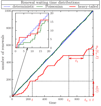
Suppose we are interested in a series of events that occur starting from time . We may later choose to specifically identify these events with the arrival of a bus, the steps of a random walk, or the blinking of a quantum dot—for now, they remain abstract. Let count the number of events that occurred up to time ; we occasionally refer to it as a counting process. The time spans between two consecutive events are called waiting times. They are not necessarily fixed. Instead, we take them to be independent, identically distributed random variables. In such a case, it is justified to refer to events as renewals: The process is not necessarily Markovian, but any memory on the past is erased with the occurrence of an event—the process is renewed. The probability density function (PDF) of individual waiting times is denoted by . Obviously, the nature of this quantity heavily influences the statistics of the overall renewal process. Figure 1 shows realizations for deterministic periodic renewals, , for Poissonian waiting times, , and for heavy-tailed waiting times, i.e. has the long- asymptotics (1). In all cases, the scaling parameter serves as a microscopic time scale for individual waiting times.
First, study the inset of Fig. 1, which focuses on the initial evolution of these processes at short time scales. The complete regularity of the deterministic renewals is distinct, but the two random counting processes are not clearly discernible by study of such single, short-period observations. Now compare this to the main figure, which depicts realizations of the processes on much longer time scales. Here, the realizations of the deterministic and Poissonian renewal processes look almost identical. Recall that for independent exponential waiting times, the average time elapsing until the th step is made increases linearly with , while the fluctuations around this average grow like . Thus, the relative deviation from the average decays to zero on longer scales. Roughly speaking, on time scales that are long as compared to the average waiting time we observe a quasi-deterministic relation .
For heavy-tailed waiting times as in (1), the picture is inherently different. Above scaling arguments fail, since the typical time scale to compare to, the average of a single waiting time, is infinite. This is why this type of dynamics are sometimes referred to as scale-free and they are studied in light of generalized central limit theorems gclt . We sketch some of the analytical aspects in the following section. Most importantly, it turns out that in the absence of a typical time scale, waiting time periods persist and are statistically relevant on arbitrarily long time scales. The effect is clearly visible in Fig. 1: The renewal process remains a nontrivial random process, even when .
We also introduce at this point the concept of an aged measurement: while the renewal process starts at time , an observer might only be willing to or capable of counting events starting from a later time . In place of the total number of renewals he then studies the counted fraction . The fundamental statistical difference between the renewal processes and stems from the statistics of the time period which passes between start of the measurement at and the observation of the very first event. We refer to it as the forward recurrence time Godreche2001 and denote its PDF by . If the observer counts starting at time , the forward recurrence time is simply distributed like any other waiting time, . But for later, aged measurements, , the distribution is different, as indicated in Fig. 1.
We call the dependence of the statistical properties of the counted renewals on the starting time of the measurement an aging effect. Its impact crucially depends on the waiting time distribution in use. For instance, a Poissonian renewal process is a Markov process, meaning here that events at all times occur at a constant rate. In this case, , so there the process does not age. For any other distribution, ; yet, if the average waiting time is finite, then on time scales long in comparison to the average waiting time , the renewal process behaves quasi-deterministically (details below). Thus aging is in effect, but becomes negligible at long times. But scale-free waiting times as in (1) result in nontrivial renewal dynamics, with distinct random properties, and aging effects should be taken into careful consideration. In the following section, we thus study and compare in detail the statistics of the renewal processes and in terms of their probability distributions and discuss the consequences for calculating aged ensemble averages.
II.2 Long time scaling limit
Several authors have studied the aging renewal process as defined above and its long time approximation, see Godreche2001 ; Bingham1971 ; Meerschaert2004 ; Hughes and references therein. We demonstrate here the basic concept of a scaling limit, focusing on the calculation of the rescaled PDF.
The probability of the random number of events taking place up to time takes a simple product form in Laplace space footnote:laplacetrafo ,
| (2) |
which is a direct consequence of the renewal property of the process. It can be read as the probability to count exactly steps at some arbitrary intermediate points in time and not seeing an event ever since, i.e. the expression is the Laplace transform of .
We also seek to study measurements taken after some time period during which the process evolved unattendedly. To this intent, we should consider , the number of events that happen during the time interval . The corresponding probability reads in double Laplace space, , Godreche2001
| (3a) | |||
| where we introduced | |||
| (3b) | |||
the PDF of the forward recurrence time as defined in the preceding section. The interpretation of Eq. (3a) is straightforward: The probability to see any events at all during the period of observation equals the probability that . Furthermore, the observer counts exactly events if the first event at time is followed by events at intermediate times and an uneventful time period until the measurement ends at .
We check that for Poissonian waiting times, , we have , and hence . The Poissonian (i.e. Markovian) renewal process is unique in this respect. We say, it does not age.
Now assume that waiting times are heavy-tailed, i.e. their PDF is of the form (1). Waiting times of this type have a diverging mean value, which has severe consequences for the resulting renewal process, even in the scaling limit of long times. To see this, introduce a scaling constant and rescale time as . Then write the following approximation in Laplace space, where, by virtue of Tauberian theorems Hughes , small Laplace variables correspond to long times,
| (4) |
If we rescale the counting process accordingly, meaning here , we can take the limit to arrive at a long time limiting version of the renewal process. For instance, the probability distribution in Eq. (2) takes the following form:
| (5a) | ||||
| Note that in these equations, was turned from an integer to a continuous variable, characterized by a PDF. Still, for simplicity, we continue to refer to this variable as ‘number of events’. For the sake of notational convenience we set in what follows, bearing in mind that the rescaled time variables and are measured in units which are by definition large as compared to the microscopic time scale of individual waiting times, the scaling factor in Eq. (1). | ||||
The evolution of the probability density with respect to real time is now given through
| (5b) |
where
| (5c) |
Remarkably, thus remains a nontrivial random quantity even after the rescaling procedure. The special limit is representative for finite average waiting times. In this case, the Laplace transform in Eq. (4) is a moment generating function, and thus we identify . In the scaling limit such a process collapses to a deterministic counting process: Eqs. (5) then imply .
In contrast, for any , obeys a scaling relation and follows a Mittag-Leffler law Bingham1971 , directly related to the one-sided stable density gclt ; footnote:plotstable . The latter is a fully continuous function on the positive half-line . This implies in particular that for , the probability to have exactly is infinitely small. Apparently, for the long time scaling limit of the counting process , the length of the very first single waiting time is negligible and the observer starts counting events immediately after initiation of the process.
The procedure for finding the PDF of counted events in an aged measurement, , is analogous. In the long time scaling limit defined above, Eqs. (3) turn into
| (6a) | |||||
| with the definition | |||||
| (6b) | |||||
| and | |||||
| (6c) | |||||
Eq. (6a) demonstrates the aging time’s distinct influence on the shape of the PDF of the number of events. Most remarkably, as , the occurrence of a term proportional to indicates a nonzero probability for counting exactly . This means that we might observe no events at all in the time interval . This is a quite distinct aging effect, contrasting the immediate increase of the non-aged counting . Only the limit leads us back to a trivial deterministic, nonaging counting process, and consequently .
For the aged PDF , Laplace inversion of Eqs. (5) and (6c) to real time yields Barkai2003a ; Barkai2003b
| (7a) | |||||
| with Godreche2001 ; Dynkin1961 ; Feller | |||||
| (7b) | |||||
| where | |||||
| (7c) | |||||
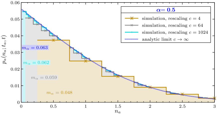
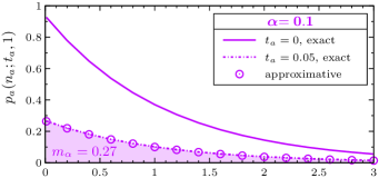
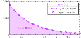
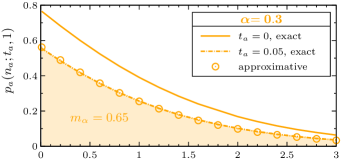
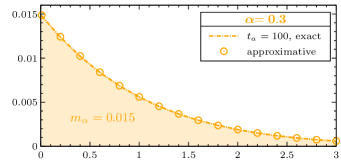
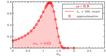
Here the asterisk indicates a Laplace convolution with respect to time . Figure 2 gives a first example of how such an aged PDF behaves. We depict the case at high ages, . In addition we demonstrate scaling convergence: if a renewal process with simple power-law waiting time distribution is monitored on increasingly long scales for time and event numbers, then its statistics approach the continuous limit described by Eqs. (7).
The latter relate the aged PDF to the non-aged PDF via the PDF of the forward recurrence time. is the probability to count any events at all during observation. Its representation in terms of an incomplete Beta function (see Appendix A) is found by a simple substitution . It can be written as a function of the ratio alone and we suggest to use the latter as a more precise and quantitative notion of the age of the measurement. In particular, we call the process or measurement or observation slightly aged, if . Conversely, we say it is strongly or highly aged, if . We now look deeper into these two limiting regimes.
II.3 Aging probability distribution
Slightly aged PDF. — First, notice that in Eqs. (7), the PDF of the forward recurrence time appears inside integrals, and should be interpreted in a distributional sense. For instance, in the limit we should recover the PDF of a non-aged system, . To confirm this, study the limit in Laplace space. We find . Thus we should write in terms of a Dirac -distribution, consistently implying and . Again we find that only an observer counting from the initiation of the (rescaled) renewal process, , witnesses the onset of activity instantly.
We can go one step beyond this limit approximation and study the properties of a slightly aged system ( and ). We write and find, by use of Tauberian theorems that
| (8) |
and
| (9a) | |||||
| Here, first order corrections are provided in terms of a Laplace inversion. For the analytical discussion, we can alternatively express them as | |||||
| (9b) | |||||
| relating them to the non-aged PDF, and thus to the familiar stable density, see Eqs. (5). Finally, we can also interpret these contributions as Fox- functions, for which we know series expansions for small arguments and asymptotics for large arguments (see Appendix A and Mathai ; the connection between Fox- functions, stable densities and fractional calculus is established in Schneider ): | |||||
| (9h) | |||||
From any of these representations, we learn that leading order corrections to the non-aged PDF are of the form . An intuitive reasoning for this can be given as follows. A slightly late observer generally has to wait for the forward recurrence time before seeing the first event. The corrections thus have to account for waiting times which start earlier than the beginning of the observation , but reach far into the observation time window . Note that the number of (still few) waiting times drawn before time is measured by , while the probability for any of them to be statistically relevant during an observation of length is proportional to . The expected number of statistically relevant waiting times starting before but reaching into the time window therefore scales like , and so do leading order corrections.
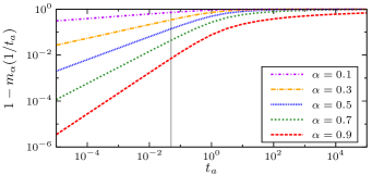
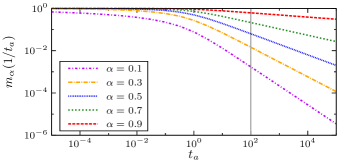
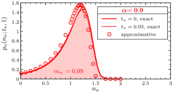
The precise nature of the modifications to the non-aged PDF due to aging can be separated into two aspects. On the one hand, the continuous part of the aged PDF, , looses weight to the discrete -part with growing age of the counting process. This reflects an increasing probability to have waiting times that not only reach into, but actually span the full observation time window, so that no events at all are observed. We provide a graphical study of the early age-dependence of , i.e. the weight of the discrete contribution, in the left panel of Fig. 3. The double logarithmic plot clearly demonstrates the initial power-law growth . Moreover we see that for any fixed age , the value of is higher for lower values of . This was to be expected, since lower values of are related to broader waiting time distributions, and thus stronger aging effects.
Interestingly, on the other hand, the modification to the continuous part of the aged PDF, , goes beyond this weight transfer: It is not proportional to the non-aged PDF itself, but, according to Eq. (9b), to its slope. With increasing age , regions with negative (positive) slope increase (decrease), so that local maxima have a tendency to shift towards . Furthermore, we can deduce from the Fox- function representation, Eq. (9h), the behavior around the origin, , and the tail asymptotics, . See Appendix A for details. For , the initial slope of is negative, and hence the early aging effect is an increase of between the origin and the local maximum. This is notable since on the long run (i.e. for sufficiently long ), the probability to have any tends to zero. For , we find the converse: the initial slope is negative, and the PDF in the vicinity of the origin starts dropping from early ages. The PDF tails are, for any value of , of a compressed exponential form, meaning here .
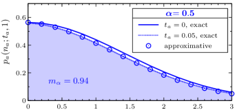
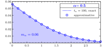
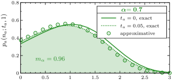
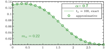
We can assess the validity of this early-age approximation by studying the left panels of Fig. 4. We plot the non-aged PDF, Eqs. (5) (full lines) footnote:plotstable , a numerical evaluation of the continuous part of the aged PDF, , as given through the full convolution integral in Eq. (7a) (dotted/dashed lines), and the early-age approximation by expanding the Fox- functions in Eq. (9h) as power series (symbols). All qualitative statements from the previous paragraph are confirmed by the sample plots. Still, the leading order approximation, Eqs. (9), is apparently not equally suitable for all values of . We observe deviations when gets close to . Indeed, one can show that the leading order terms in Eqs. (9), which account for corrections of , are followed by higher order terms of . Hence, in general, these ‘almost leading order’ corrections need to be taken into account when is close to 1. Yet again, in this case, the total corrections with respect to the non-aged PDF, as measured in terms of the weight loss , are relatively small anyway.
Highly aged PDF. — Conversely, we approximate for : . This yields the leading order behavior for highly aged measurements, :
| (10) |
and
| (11a) | |||
| Above Laplace inversion can be related to the non-aged PDF (5) through | |||
| or expressed as Fox- function by | |||
| (11e) | |||
Again, modifications account for waiting times that start before but reach into the time window of observation. But in this late time regime, the initiation of the renewal process already lies far in the past, so not all waiting times before have a realistic chance to do that. Instead, we assume again that statistically relevant pre-measurement waiting times need to be of the order of (implying a probability ). To estimate their number, note that they must follow events which occur roughly within a time period . However, at this (late) stage of the renewal process, the average event rate has dropped to . Thus the expected number of waiting times in the (comparatively short) time period preceding the measurement we conjecture scales like . This heuristic line of argument explains why for highly aged measurements, we have leading order contributions of the order .
Graphical examples for this regime are given in the right-hand panels of Figs. 3 and 4. Here, the continuous part of the aged PDF is not proportional to the slope of the non-aged PDF, but, according to Eq. (LABEL:renewal:aPDF_high_invstabl), rather its time integral over the duration of the measurement. Moreover, through its Fox- function representation (11e), we learn that the initial slope of the late age PDF is positive for and negative if . The far tail behavior however persists at late aging stages, as we still find . Notice that in the case of high ages, in Fig. 4 realized as , the leading order terms (11a) are satisfactorily approximating the exact convolution (7a) for all values of .
II.4 Aging ensemble averages
From the non-aged PDF in Eq. (5a) one can derive the expected time behavior of any function of the number of events counted since the initiation of the renewal process:
| (12) |
We give concrete examples below. First, we ask how such an ensemble average is altered if evaluated for the aged counting process. For this, we substitute by and by and insert Eqs. (7) to (11):
| (13a) | |||
| with the limiting behavior | |||
| (13b) | |||
These equations relate an ensemble average taken for the observation window to the respective quantity measured in . Interestingly, the modifications due to aging are rather related to the ensemble average of the derivative of the observable, .
As an example we consider th order moments of the number of renewals, , . We find
| (14a) | |||||
| and | |||||
| (14d) | |||||
| The incomplete Beta function comes into play again by substituting in the convolution integral in expression (13a). The time-independent coefficients are given by | |||||
| (14e) | |||||
For the non-aged system, moments evolve like , reflecting the characteristic scaling property of the renewal process, . But for aged systems, , the scaling is broken, and moments behave in a more complex fashion with respect to time. Only at very high ages, , we can approximate again by a single power-law. When comparing the growth of the counting processes for the two limiting regimes, Eq. (14d) is somewhat ambivalent. At high ages, the probability for observing no events at all tends to one. Consequently, a prefactor lets all moments decay to zero as goes to . However note that for a fixed, large but finite value of , the -dependence is (in accordance with Meroz2010 ), so the power-law exponent is actually larger than for the non-aged moments. In summary, at higher ages , the absolute number of counted events drops, but it increases faster with measurement time . In particular, consider the average number of events during observation, : Counting from the start of the process, we observe a sublinear behavior ; but at fixed, high age of the process, the average rate of events is approximately constant, , like in a nonaging, Poisson type of renewal process.
Another useful expression is the Laplace transform of Eq. (5a) with respect to the number of renewals, , and respectively Eq. (6a) with , which is obtained through the same techniques. Thus,
| (15a) | |||
| and | |||
| (15b) | |||
where and are (generalized) Mittag-Leffler functions (see Appendix A). Interestingly, here the early first order corrections due to aging do not significantly alter the -dependence. At low age, the Mittag-Leffler function interpolates between for and at . At high age, the transition is from to .
II.5 Conditional ensemble averages
To conclude this section, we address the question of how counting statistics change when we selectively evaluate only realizations of the process where . This means we discard the data when no events happen during the complete time of observation . This is, on the one hand, a relevant question when it comes to the application of renewal theory: An observer who is unaware of the underlying counting mechanism, might misinterpret realizations with as a separate, dynamically different process, since the statistics are so distinct from the remaining continuum . A process realization during which no events occur at all might even not be visible to the observer in the first place. We give an example in the next section. On the other hand, this study also helps us to distinguish two aspects of the aging PDF: We neglect the effect of having single waiting times that cover the full observation window, leading to a weight transfer from the continuous to the discrete part of the PDF. Instead we specifically only account for waiting times that start before but finish during the period of observation, in order to understand the modifications of the continuous part beyond its loss of weight. To this intent, we look at the conditional ensemble average
| (16) |
For , as mentioned above, counting of events starts instantly, so the restriction to is redundant. But in the limit of late ages, a possibly nonzero forward recurrence time affects the measurement. We find that ensemble averages conditioned to have a well defined, nontrivial limiting time dependence, even when tends to infinity. This is in contrast to the full ensemble, where at infinite ages, . As an example consider again the time evolution of th order moments, restricted to . We find
| (17a) | |||
| but | |||
| (17b) | |||
| where is given by Eq. (14e) and | |||
| (17c) | |||
Thus, as opposed to the unrestricted ensemble measurement, conditional moments scale like in both non-aged and extremely aged systems. Note however, that prefactors are different, and a behavior deviating from a simple power-law is still observable at intermediate ages.
III Aging continuous time random walks
The theory of continuous time random walks (CTRWs) directly builds on the concept of the renewal theory. We are thus able to view many of the intriguing features of this random motion, such as anomalous diffusion, population splitting and weak ergodicity breaking, in the light of the abstract analytical renewal theory ideas developed above. To do so, we start with a definition of the CTRW model in section III.1, extending the renewal process by a random spatial displacement component. We then review results from previous work in the field, discussing in particular the aspects of population splitting (section III.2), anomalous diffusion and weak ergodicity breaking (section III.3). Concurrently, we add elements from our own recent discussion Schulz2013 , aiming at relating these phenomena to the aging properties of the underlying renewal process. Population splitting can be traced back to the partially discrete nature of the aging renewal PDF. Studying ergodicity ultimately leads us to a general in-depth study of aging ensemble and time averages (section III.4). We work out the fundamental differences between these two types of averages under aging conditions (weak ergodicity breaking), but also find interesting parallels at late ages (equivalence in time scalings). Finally, we apply the methods and formulae developed in the course of our discussion to analyze a stochastic process which generalizes previous CTRW models by additional confinement, friction and memory components in section (III.5).
III.1 From aging renewal theory to aging continuous time random walks
Consider a random walk process (one dimensional, for the sake of simplicity) in which steps do not occur at a fixed deterministic rate, but are instead separated by random, real valued waiting times. The idea is to model the random motion in a complex environment where sticking, trapping or binding reactions are to be taken into account. The processes we study here are CTRWs with finite-variance jump lengths on the one hand, and independent, identically distributed waiting times on the other (see report ; Hughes for a review on CTRW theory). Eventually we are interested in studying these processes on long time scales, aiming at extending existing simple diffusion models to describe diffusion in complex environments. Thus, we focus again on scale-free waiting time distributions of the form (1), which have the capability of modifying the resulting diffusion dynamics on arbitrarily long time scales.
In the simplest scenario, sticking or trapping mechanisms are decoupled from diffusion dynamics. On the level of theoretical modeling, this means we can take jump distances of the base random walk to be independent from waiting times. The renewal theory of the previous section is readily extended to describe such idealized systems. Let be the random walk process as a function of the number of steps . Then by means of subordination Meerschaert2004 ; Fogedby1994 ; Baule2005 ; Magdziarz2007 , we construct a CTRW as , where is a renewal counting process. Each step of the random walk is hence interpreted as an event of the renewal process. The properties of follow from the combined statistics of and . For example, if denotes the PDF for the position coordinate after steps, starting with , then
| (18) |
is the PDF of the associate CTRW process at time . Note that we see as a continuous variable here, so we are arguing on the level of long time scaling limits. In the simplest case, would be an ordinary Brownian motion so that would be a Gaussian.
Now imagine that a particle is injected into a complex environment, beginning a CTRW like motion at time . In general, the experimentalist might start its observation at a later time . The reason for this could be experimental limitations, or maybe the goal is to study a maximally relaxed system, which makes it necessary to wait for relaxation. In either case, the particle motion is initially unattended. At time the particle is tracked down, and its position at this instant serves as the origin of motion for the following observations. Instead of the full CTRW , the experimentalist then monitors the aged CTRW . Thus, as we worked out in the previous section, if the dynamics are characterized by heavy-tailed trapping or sticking times, the issue of aging has to be taken into careful consideration.
III.2 Population splitting
Arguably the most striking aging effect in CTRW theory is the emergence of an apparent population splitting Schulz2013 ; Barkai2003b . The aged renewal process controls the dynamic activity of the aged CTRW . Consequently, the forward recurrence time marks the onset of dynamic motion in the monitored window of time. We learned from the analysis of aging renewal theory that for increasingly late measurements, we should expect to assume considerable values. Physically, this reflects the possibility for the particle to find ever deeper traps or to undergo more complex binding procedures, when given more time to probe its environment before the beginning of observation. In particular, the forward recurrence time is more and more likely to span the full observation time window, , so that the particle does not visibly exhibit dynamic activity.
From an external, experimental point of view, an ensemble measurement in such a system appears to indicate a splitting of populations. Let, for instance, the base random walk be Markovian, and let the PDF be a continuous function of (e.g. Gaussian). In this case we can supplement the ensemble PDF from Eq. (18) by its aged counterpart , using renewal theory Eq. (13a):
| (19) |
This propagator was discussed previously in Barkai2003b . The ensemble statistics have a sharply peaked -contribution, caused by a fraction of particles which remain immobile at the origin of the observed motion. They contrast the mobile fraction of particles, since the PDF of their arrival coordinates, , varies continuously along the accessible regions of space (as derived, by virtue of Eq. (18), from the continuous nature of the PDFs , and ). For fixed evaluation time , the size of the immobile subpopulation increases with growing age , as aging renewal dynamics terminally come to a complete halt. An exhaustive discussion on the shape of the aged propagator can be found in Barkai2003b for both unbiased motion and in the presence of a drift.
Indeed, splitting into subpopulations is a phenomenon encountered in complex environments such as biological cells. Such dynamics was observed for the motion of lipids in phospholipid membranes Schutz1997 , single protein molecules in the cell nucleus Kues2001 , H-Ras on plasma membranes Lommerse2005 , and of membrane proteins Manley2008 . The immobile fraction is also often found in fluorescence recovery after photobleaching experiments Schutz1997 .
It is important to understand, that for CTRW types of motion, this effect emerges without assuming non-identical particle dynamics. Even during the evolution of the process, stochastic motion of individual particles in an ensemble is independent and identical. In particular, all particles in principle exhibit their dynamic activity for an indefinite amount of time. The ‘immobility attribute’ can only be assigned when the evolution of the (aged) process is studied within a finite time window. Then, a certain fraction of particles—the immobile ones—stand out statistically from the rest. The displacement propagator (19) with its conspicuous, discontinuous contribution serves as a statistical indicator for the population splitting, if evaluated at finite times (more precisely, the effect is most noticeable while remains short as compared to the age ). Similarly, we show in the following section that population splitting is particularly relevant when assessing time average data on a per-trajectory basis. Of course, in any case, observations of real physical systems are finite by nature. It is hence important to know the characteristics of the aging population splitting, as to set it apart from separation mechanisms due to physically non-identical particle dynamics.
III.3 Analysis of mean squared displacements
An alternative way to assess particle spreading in the solvent is to study the time evolution of the mean squared displacement. This is particularly useful when ensemble data is not extensive enough as to deduce reliable propagator statistics . There are two common ways of defining such mean squared displacements: either in terms of an ensemble average or a single-trajectory time average. Analysis and comparison of these two types of observables reveals several fingerprint phenomena of CTRW motion, such as subdiffusion and weak ergodicity breaking. In the following, we collect known results and discuss their implications for aged systems.
Ensemble average. — As a simple example, we take to be unbounded, unbiased Brownian motion and consider an ensemble measurement of the mean squared displacement. In this case, the PDF is Gaussian, and we know that
| (20) | |||||
for all . We use arbitrary spatial units from here, . Since is a process with stationary increments, the calculation of moments is independent of the number of steps made before start of the measurement. Thus, if the process the experimentalist studies is Brownian motion, there are no aging effects: at all initial times , one observes a linear scaling with respect to observational time , , a behavior commonly classified as normal diffusion. However, if the motion is paused irregularly for heavy-tailed waiting time periods, the dynamics are of CTRW type and we get a quite different picture. For the process , we find
| (23) | |||||
in accordance with Barkai2003b . As expected, the nonstationarity of the aging renewal process carries over to the CTRW. If monitored at , the mean squared displacement grows like . With the increase being less than linear in time, the phenomenon in the context of diffusion dynamics is commonly referred to as subdiffusion. For , the mean squared displacement is no longer described in terms of a single power-law. The process looks more like diffusion in a nonequilibrium environment and in fact might be conceived as an internal relaxation time scale. Interestingly, if the measurement takes place in the highly aged regime , the mean squared displacement as a function of the observation time indicates normal diffusion with an age dependent diffusion coefficient, . Only if data on an extensive range of time scales is available, we are able to identify the complete turnover from one aging regime to the other as a fingerprint of CTRW dynamics. Still, for as long as the experimentalist cannot control the age of the measurement, the aging effect can be misinterpreted as an internal relaxation mechanism. The situation gets even more complicated, when is possibly random.
Time average. — Now consider the alternative time average notion of the mean squared displacement. For a single particle trajectory , recorded at times , it is defined in terms of the sliding average
| (24) |
Here, is called lag time, and parameters defining the time window of observation are also referred to as age and measurement time . While the ensemble mean (23) is evaluated in terms of squared displacements from a multitude of independent process realizations, the time average (24) uses data from within a single trajectory at several points in time. The latter is thus a useful alternative whenever measurements on long (i.e. ) but relatively few trajectories are available. For ergodic, stationary processes, both types of averages are equivalent. For example, for a Brownian motion, the time average is by definition a random quantity differing from one trajectory to the next; but in the limit of long trajectory measurements, , the time average converges to the corresponding ensemble value, , and fluctuations become negligible Burov2010 .
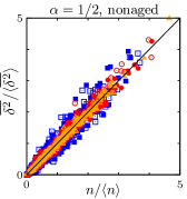
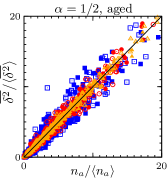
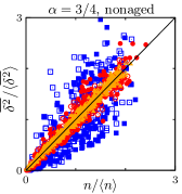
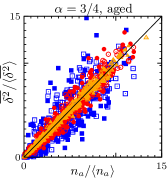
In contrast, the CTRW violates both ergodicity ( remains random for arbitrarily long measurement times) and stationarity ( depends on and ). In the context of aging, we can now ask two questions. First, does the distribution of the time average change qualitatively when evaluated after the onset of the particle dynamics, ? This issue is discussed extensively in Schulz2013 . In short, we find that the time averaged mean squared displacement is directly related to the number of steps made during the measurement via He2008 ; Burov2010 ; Jeon2010
| (25) |
Figure 5 provides a numerical validation of this relation in terms of explicit CTRW simulations for free and confined motion. Notice that Eq. (25) is not a distributional equality, but meant to be a stronger, per-trajectory equality which we validate here by means of simulations data. Hence, all random properties of the time average in this case are not only related to, but quite literally taken over from the underlying counting process. In particular, the distribution of the time average is a rescaled version of the renewal theory PDF as discussed in section II and plotted in Figs. 3 and 4. This implies that a statistical study of time averages reveals the aging population splitting: within an ensemble of independent particles, we may find some which do not exhibit any dynamic activity during observation, or , and thus apparently stand out as an individual subpopulation from the remaining continuum, or . Likewise, one can study Albers2013 the statistics of microscopic diffusivities along a single time series . These diffusivities are consistently found to have a discrete probability for . The latter implies that no steps are made during any -sized lag time interval along the time series, and the probability for this actually grows with measurement time .
The second aging-related question addresses the explicit lag time dependence. Albeit being different from one trajectory to the next, is generally characterized by a universal scaling with respect to lag time . The question now is: Is this scaling age-dependent? To this end, we consider the average (over many individual trajectories) of Eq. (24). By help of Eq. (23),
| (26a) | |||
| where | |||
| (26b) | |||
The approximation in the fourth line is for the relevant case of long measurement times, . A few points are remarkable when comparing the time dependence of the ensemble average, Eq. (23) to the scaling of the time average, Eq. (26a). The answer to the question on the lag time dependence is a simple one: We generally find a linear scaling , regardless of age . In this respect, the time average is a less complicated observable than the ensemble average. The latter has a comparatively complicated -dependence and is characterized by an age-dependent regime separation. Compare this to the time average, where nonstationarity enters in terms of the prefactors and . Only the amplitude of time averages depends on the measurement duration and age. More precisely, if either measurement time parameter tends to , the time average itself tends to zero. This is why we call an aging depression. It can be expressed in terms of the dimensionless ratio . In analogy to ensemble measurements we thus speak of a non-aged (), a slightly aged () and a highly aged () time average.
Aside from the differences, there is also an interesting parallel between ensemble and time averages: the linear scaling of the time average with respect to is reminiscent of the linear -dependence of the ensemble average at high ages. If, in addition to a very long measurement duration, we also assume an even longer preceding aging period, , the similarity even becomes an equivalence,
| (27) |
The time scalings of ensemble and time averages are hence identical at high ages. This is quite surprising considering that these quantities are fundamentally distinct in a process that exhibits weak ergodicity breaking. In what follows, we discuss whether or not these discrepancies and parallels of the two types of averages are specific to the mean squared displacement.
III.4 Aging ensemble and time averages
Consider a random walk and a stationary observable , meaning that
| (28) |
for any number of steps or . In other words, the above ensemble average should not depend on when we begin the observation. The example discussed in the previous section falls into this category. There, was Brownian motion, was the squared displacement, and we had . But condition (28) would also allow for general order moments or any other function of displacements . Moreover, we can replace by other processes with stationary increments, like fractional Brownian motion Mandelbrot1968 . If is even stationary itself (e.g. the stationary limit of confined motion), then any function is fine (allowing to calculate, e.g. correlation functions, ; CTRW multi-point correlation functions have been studied extensively in Baule2005 ; Sanda2005 ; Barkai2007 ; Burov2010 ).
Ensemble averages. — In any such case, we can ask the question of how the statistical properties of the random motion and the measured observable change when introducing heavy-tailed waiting times between steps. We define via subordination, assuming that and are stochastically independent processes. In general, the aging properties of the renewal process are inherited by the CTRW . The stationarity of the ensemble average is broken. To calculate the magnitude of the effect, we can use conditional averaging by virtue of the independency of the two stochastic processes at work. We denote by the average with respect to realizations and write
| (29a) | ||||
| The average on the last line is with respect to , so we can use our knowledge on ensemble averages of the aging renewal process. The latter are characterized by a distinct turnover behavior, see Eqs. (12) and (13b). For the slightly aged CTRW ensemble average, we have | ||||
| (29b) | ||||
| For CTRWs, the leading order corrections due to aging are of the order , just as for the underlying renewal process. Conversely, at high ages, we slightly rewrite the leading order terms as | ||||
| (29c) | ||||
introducing the constant and defining an auxiliary function , either relating it to the analog stationary average (third line) or to the corresponding non-aged CTRW average (second line). When the measurement of the observable is taken arbitrarily late, , we will ultimately measure the constant . For example, if the base random motion is a random walk with a characteristic scaling , , and we study moments of displacements, , , then ; in this case, , so we will get arbitrarily small moments at high ages. If is the stationary limit of a confined motion and we are interested in the correlation function (as studied in Burov2010 ; Schulz2013 ), then late measurements will be close to the thermal value of the squared position . The decay to this constant value is generally of the order , no matter which observable we are studying.
Time averages. — Now we turn to the analog time average, namely
| (30a) | |||||
| and calculate its expectation value | |||||
| (30b) | |||||
The approximation in the second line holds for sufficiently long trajectories, . Notice that from the full, possibly complicated time dependence of the ensemble average, only the late-age limiting behavior, Eq. (29c), entered this approximation. The reason is that with the integrand in the time average of Eq. (30b) decaying like , the integral itself is still an increasing function of , namely it grows like .
Thus, indeed aging effects for time averages in CTRW type of random motion are universally described in terms of the constant and simple prefactors and . The full lag time dependence is captured by the function , which is independent of the parameters defining the time window of observation, and . Conversely, the concrete choice for the model or the observable enter only and , but not the prefactors.
Furthermore, the -dependence of the time average is closely related to the -dependence of the ensemble average at high ages, . In particular, we find a universal asymptotic equivalence in the time scaling of time and ensemble averages, if both are taken during late measurements:
| (31) |
Thus indeed, averaging at late ages appears to happen under stationary conditions. Keep in mind however, that above identity refers to the expectation value of time averages, and thus to the time scaling behavior. Since CTRWs exhibit weak ergodicity breaking, the amplitude of the time average of a single trajectory can largely deviate from the expected value, especially at high ages, See for instance the discussion on the ergodicity breaking parameter for in Schulz2013 .
III.5 Interplay of aging and internal relaxation
To conclude the section on aging CTRWs, we study a process which extends the previous examples to a more elaborate model. On the one hand, this serves as exemplary application of the formulae and methods described in this paper. In particular, it gives a concrete meaning to the analytical discussion of time and ensemble averages and their relation to internal relaxation time scales. On the other hand, its complexity and versatility makes it more suitable for possibly describing real world physical phenomena (examples below). The definition of the model is as follows.
With our base random walk we depart from the simple Brownian motion and instead consider the fractional Langevin equation (FLE)
| (32) |
Here, the dot signals a first order derivative, is a generalized friction constant, gives the thermal energy of the environment, and quantifies the strength of an external, harmonic potential , centered around . Thus, this FLE describes the random motion of a point-like particle subject to the static external potential, a friction force, and a fluctuating force due to the interaction with the surrounding heat bath. We assume that dynamics are overdamped, meaning that the particle mass is so small that we can neglect particle inertia. Consequently, there is no term proportional to in Eq. (32). The random force is modeled in terms of the so called fractional Gaussian noise, i.e. a Gaussian process defined through Mandelbrot1968 ; Gripenberg1996
| (33a) | |||||
| and | |||||
| (33b) | |||||
where .
While the noise process itself can be defined, in principle, for any , the friction kernel in Eq. (32) diverges for values . Hence, we restrict ourselves to , implying that noise correlations are of the long-range, persistent type. They stand for the interaction with a complex environment, where relaxation dynamics are slow and cannot be characterized in terms of single relaxation rates. The latter anomalous diffusion phenomenon comes about when accounting for obstructed motion (e.g. single-file diffusion Sander2012 or other many-body systems Lizana2010 ; Kupferman2004 ) or an interaction with a viscoelastic network Goychuk2012 ; Weber2010 . Biological cells feature highly complex, crowded environments, crossed by filament networks. FLE dynamics have thus found wide application in biological physics, describing diffusive motion processes within the cell Weber2010 ; Burnecki2012 ; Szymanski2009 ; Jeon2012a , but also conformational dynamics of individual protein complexes Min2005 .
Such long-range correlations carry over to the particle motion in a two-fold way, as also the friction term in Eq. (32) incorporates long-range memory effects: its magnitude is defined by the complete velocity history starting from . The power-law memory kernel is chosen such that this FLE fulfills a Kubo-style fluctuation dissipation theorem Kubo1966 . This implies that deterministic friction and random noise forces do not originate from separate physical mechanisms, but are both generated by interactions with the environment. Moreover, it means we can model ‘equilibrated diffusion’: Eq. (32) admits a solution with a stationary velocity profile, so that the net energy exchange of the particle with the heat bath is zero. Such a solution is a Gaussian process defined by Pottier2003
| (34a) | |||
| and | |||
| (34b) | |||
in terms of a generalized Mittag-Leffler function (appendix A), introducing . (Note that the definition of a Gaussian process in terms of its correlation function is equivalent to the definition in terms of squared increments, since .) The nonequilibrium solutions to the FLE are discussed in Deng2009 ; Kursawe2013 , including an interesting discussion on their transient aging behavior Kursawe2013 . In the limit , Eq. (34b) defines a stationary Ornstein-Uhlenbeck process, implying exponential relaxation. Physically, the latter models overdamped motion in an harmonic potential where friction and noise forces are memoryless.
The stationary Gaussian process (34b) is the starting point for our discussion on aging induced by heavy-tailed waiting times. There are, of course, various ways to introduce an aging, nonergodic, CTRW-like model component, and the resulting stochastic processes differ largely. For instance, one can combine the Gaussian dynamics with an independent CTRW motion in a purely additive manner, as discussed in Jeon2013a . Moreover, for a nonoverdamped, inertial motion, the FLE velocity process can be modified by adding periods of constant velocity with heavy-tailed statistics Friedrich2006 . Here, we instead stick to the standard subordination approach as described in the preceding sections: we introduce stalling dynamics by defining , where the aging renewal process is assumed to be statistically independent from . Physically, this scenario implies that the particle under observation is governed by the FLE (32). Eventually, it becomes trapped for a random waiting time controlled by the probability density . After release from the trap we assume that the particle motion quickly thermalizes and the particle again follows the stationary Gaussian dynamics (34b) until the next trapping event.
We basically have three motivations to study this random motion. First, CTRWs provide one approach to model diffusive motion in biological cells, where waiting times represent multi-scale binding or caging dynamics. The sheer complexity of this kind of environment however brings the necessity to further introduce aspects of anomalous diffusion not contained in the renewal process cells ; Meroz2010 ; Akimoto2011 ; Weiss2013 ; Tabei2013 ; Hoefling2013 . While the overdamped FLE dynamics (34b) adds both friction and external binding forces, it also introduces the concept of long-time correlations within an equilibrated environment.
From the point of view of our theoretical discussion of aging CTRWs, our second motive to discuss this particular model is the stationarity of increments of . It allows us to exercise the methods we introduced in the previous section by calculating ensemble and time averages—mean squared displacements in particular—of the aging process .
Third, aside from its didactic purpose, the definition of the process also extends the ordinary Brownian motion by introduction of an intrinsic time scale , characterizing the competition between binding and friction forces. According to Eq. (34b), stationary Langevin dynamics exhibit a turnover
| (35) |
from subdiffusion on short time scales to the stationary Boltzmann-limit on long scales. Now for the aging process , we know that the age of a measurement itself can be conceived as a time scale separating the time dependence into early and late age behavior. It would be interesting to know how complex the process behaves with respect to both time scales. Are all conceivable time regimes clearly distinct? Are time and ensemble averages equally sensitive to transitions from one regime to the other?
A partial answer is given by Eqs. (29c), which focus on the calculation of ensemble averages. We discuss the mean squared displacement, and as defined through Eqs. (34b). Inserting the latter into Eq. (29b), we find an approximation for low ages, :
In order to obtain reasonable physical units, we reintroduced the parameter from Eq. (1) bearing the dimension of seconds. Moreover, the new constant has physical units .
For increasingly aged ensemble measurements, aging corrections of the order come into play. The detailed time behavior of the ensemble mean squared displacement is found by combining Eqs. (34b), (29a) and (13a). We here have , and thus we can write
| (37a) | |||
| The full time dependence of the ensemble average comes as a convolution of the forward recurrence time PDF (7c) with a generalized Mittag-Leffler function. We provide graphical examples below. | |||
The behavior at high ages, can be calculated analytically by use of Eqs. (34b) and (29b), yielding
| (37b) |
where in this case and
| (37c) | |||||
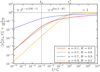
The time dependence of the mean squared displacement, Eq. (37a), is relatively complicated. In both the limits of slightly and highly aged measurements we observe a Mittag-Leffler behavior, but with different parameters. We can extract from Eqs. (III.5) and (37c) four time regimes where the diffusive behavior with respect to time is described in terms of single power-laws; regimes are separated by a time scale induced by aging and an intrinsic relaxation time scale ,
| (38a) | ||||
| with coefficients | ||||
| (38b) | ||||
Figure 6 gives several examples for the detailed turnover behavior of the mean squared displacement for various values of and . At infinite times , the ensemble mean squared displacement converges to the Boltzmann limit. At finite times, we generally observe subdiffusive behavior. The dynamics are slowest when is short as compared both intrinsic relaxation and aging time scales. Notice that the behavior at times is independent of the parameter defining the memory of friction and noise forces. This regime is fully dominated by the aging transition.
Again we stress that the full double turnover behavior of the ensemble average might not be visible to the observer of a real physical system due to limitations of the experimental setup. In addition, precise knowledge on the aging time , which preceded the actual ensemble measurement, might not be available. Maybe is even random, varying from one trajectory to the next. In any such case, the observer cannot know which of the power-law regimes of (38a) he is probing by means of mean squared displacement measurements.
The analog time average measurement is much less complex and thus easier to interpret. According to Eq. (30b) we have for ,
| (39) |
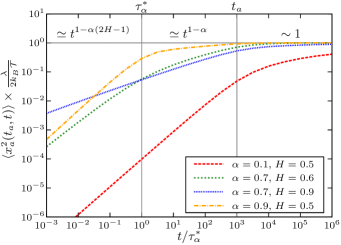
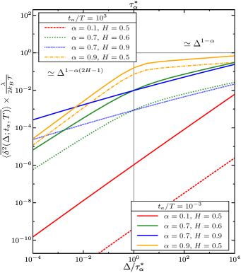
The dependence on age and measurement time parameters, and factorizes from the lag time dependence. The latter is captured by the function . Recall that for weakly nonergodic CTRW dynamics, the amplitude of a single-trajectory time average is random by nature, while its scaling with lag time is not. Thus, the -scaling of the time averaged mean squared displacement is age-independent. For combined CTRW-FLE dynamics, it is universally given by in terms of a Mittag-Leffler type single turnover, with (lag) time regimes being separated by the intrinsic time scale . In particular, a single, long trajectory measurement is in principle sufficient to read off the scaling exponents and , and the time scale .
Aging affects the amplitude of the time average only: as increases, we expect smaller values of . For exemplary plots, see Fig. 7. Notice that the late lag time behavior is generally , independently of , as reported previously Neusius2009 ; Burov2010 for confined, memoryless CTRWs (i.e. for ). Moreover, in the limit , aging becomes negligible, , and we recover the ergodic FLE result , with as in Eqs. (34b).
IV Conclusions
We investigated a renewal process in which the average waiting time between consecutive renewals is infinite. For such a process, randomness is relevant on even the longest of time scales. We worked out several nontrivial properties, and here we concentrated on the phenomenon of aging: the statistics of renewals counted within a finite observation time window strongly depends on the specific instant at which we start to count. The most remarkable aging effect is a growing, discrete probability to not count a single event during observation. Concurrently, also the continuous distribution of the nonzero number of renewals is transformed. We discussed analytical expressions for this distribution with respect to series expansions, tail behavior and monotonicity, see Eqs. (9) to (11) and Figs. 3 and 4. We deduced exact expressions for related ensemble averages, Eqs. (13b), such as arbitrary moments of the number of renewals in terms of incomplete Beta functions, Eq. (14d). We found that we count fewer renewals at increasingly late ages. However, this is mainly due to the high probability of counting zero renewals. Restricting the counting statistics to eventful measurements, see Eq. (17b), yields a finite distribution even at infinite age, characterized by the same time scaling as the non-aged process.
We applied this aging renewal theory to CTRW models: renewal events are identified with steps of the random walk. The aging effects translate from the renewal to the random walk process. Thus the increasing probability for the complete absence of dynamic activity is conceived as a population splitting effect. In an ensemble of identical particles, a certain fraction remains fully immobile during a finite time observation. The total size of the mobile population decreases with age, but also their detailed statistics change.
We discussed the implications for ensemble and time averaged observables in CTRW theory. Aging affects the distributions of time averages, and population splitting has to be considered in particular. Remarkably, we find that ensemble averages behave very differently with respect to aging effects than the analogous time averages. The age of a measurement modifies the complete time dependence of an ensemble average, mimicking an internal relaxation mechanism. We provide an analytical description in terms of Eqs. (29c). In contrast, aging enters the associate time average only as a distributional modification, while its scaling with respect to (lag) time remains indifferent. We calculated the respective scaling function [see Eqs. (29c) and (30b)]. In addition, we derived the precise aging modifications for the ensemble averaged time average. The latter in turn do not depend on details of the definition of the process or the observable. Instead they are captured by universal constants, and the age enters in particular through the aging depression , defined in Eq. (26b). Despite this fundamental conceptual difference between time and ensemble averages, we found that their time scalings are identical in highly aged measurements. This is a surprising result since CTRWs are notorious for weak ergodicity breaking, i.e. the general inequivalence of the two types of averages.
We bestowed a more specific meaning to these general considerations by discussing combined FLE-CTRW dynamics. The latter extend ordinary CTRW models by introduction of binding and friction forces and a correlated noise. We contrasted turnover behaviors of aging and internal relaxation, and gave a detailed discussion of associated limiting regimes.
The CTRW is a very natural application of aging renewal theory, yet it is far from unique. All aging effects such as population splitting and altered ergodic behavior have their analog phenomenon in any physical system where the mean sojourn time in microstates is infinite. Thus we expect a certain fraction of blinking quantum dots, or cool atoms, to be constantly stuck in one state during a delayed observation period. At the same time the statistics of the switching population are aging. Power spectral densities obtained from signals from such systems should display related aging properties, as discussed briefly in Niemann2013 . Aside from stochastic process studies, also weakly chaotic systems were shown to exhibit analogous aging behaviors Akimoto2013 . When it comes to diffusion dynamics, a study of alternative CTRW-like models might turn out worthwhile. Examples are the noisy CTRW Jeon2013a , aging renewals on a velocity level Friedrich2006 , Lévy walks Shlesinger1987 , non-renewal, correlated CTRW Tejedor2010 , and aging CTRW lomholt . Moreover, further studies of the aging renewal process, e. g. with respect to higher dimensional probability distributions, will reveal additional insight into aging mechanisms of such physical systems.
Acknowledgements.
Johannes Schulz was supported by the Elitenetzwerk Bayern in the framework of the doctorate program Material Science of Complex Interfaces. We acknowledge funding from the Academy of Finland (FiDiPro scheme), and the Israel Science Foundation.Appendix A Special functions
The asymptotics of the PDF of the aging renewal process , Eqs. (9h) and (11e), and the rescaled TAMSD distribution in Eq. (25) for highly aged processes contain the Fox -function, a very convenient special function Mathai . For the specific cases considered here the series expansion around is
| (40) |
The behavior for large values of is stretched exponential,
| (41) |
with the abbreviations
| (42) |
Logarithmic tail analysis thus yields
| (43) |
independently of . The expressions for as non-aged, slightly aged and strongly aged renewal PDF are obtained by substituting with , and , respectively. Note that for the relevant -functions simply become
| (46) | |||||
| (49) | |||||
| (52) |
in terms of exponential and complementary error functions.
The probability in Eq. (7a) and the th order moments of renewals (14d) are expressed in terms of an incomplete Beta function, defined through Abramowitz
| (55) | |||||
with the special value
| (56) |
Here and .
The Laplace transform of with respect to the number of events, Eqs. (15a) and (15b), and the mean squared displace for FLE motion, Eqs (34b), (III.5) and (37c) are expressed in terms of generalized Mittag-Leffler functions. The latter are characterized alternatively by series expansions around ,
| (57) |
asymptotic series for large arguments,
| (58) |
or by their Laplace pair
| (59) |
for any . The ordinary Mittag-Leffler functions are the special cases .
References
- (1) D. Cox, Renewal Theory (Methuen & Co., London, 1970).
- (2) F. Bardou, J.-P. Bouchaud, A. Aspect, and C. Cohen-Tannoudji, Lévy Statistics and Laser Cooling (Cambridge University Press, Cambridge, England, 2002); F. Bardou, J.-P. Bouchaud, O. Emile, A. Aspect, and C. Cohen-Tannoudji, Phys. Rev. Lett. 72, 203 (1994) .
- (3) E. Lutz, Phys. Rev. Lett. 793, 190602 (2004).
- (4) X. Brokmann, J.-P. Hermier, G. Messin, P. Desbiolles, J.-P. Bouchaud, and M. Dahan, Phys. Rev. Lett. 90, 120601 (2003) .
- (5) G. Margolin and E. Barkai, J. Chem. Phys. 121, 1566 (2004).
- (6) K. T. Shimizu, R. G. Neuhauser, C. A. Leatherdale, S. A. Empedocles, W. K. Woo, and M. G. Bawendi, Phys. Rev. B 63, 205316 (2001).
- (7) J.-P. Bouchaud, J. Phys. I (Paris) 2, 1705 (1992).
- (8) H. Scher and E. W. Montroll, Phys. Rev. B 12, 2455 (1975).
- (9) J.-H. Jeon, V. Tejedor, S. Burov, E. Barkai, C. Selhuber-Unkel, K. Berg-Sørensen, L. Oddershede, and R. Metzler, Phys. Rev. Lett. 106, 048103 (2011); A. V. Weigel, B. Simon, M. M. Tamkun, and D. Krapf, Proc. Nat. Acad. Sci. USA 108, 6438 (2011).
- (10) A. Rebenshtok and E. Barkai, J. Stat. Phys. 133, 565 (2008).
- (11) C. Godrèche and J.M. Luck, J. Stat. Phys. 104, 489 (2001).
- (12) E. Barkai, Phys. Rev. Lett. 90, 104101 (2003).
- (13) E. Barkai and Y.-C. Cheng, J. Chem. Phys. 118, 167 (2003).
- (14) B. D. Hughes, Random Walks and Random Environ- ments, Vol. I: Random Walks (Oxford University Press, Oxford, UK, 1995).
- (15) R. Metzler and J. Klafter, Phys. Rep. 339, 1 (2000); J. Phys. A 37, R161 (2004).110
- (16) C. Monthus, and J.-P. Bouchaud, J. Phys. A 29, 3847 (1996)
- (17) J. H. P. Schulz, E. Barkai, and R. Metzler, Phys. Rev. Lett. 110, 020602 (2013).
- (18) Y. He, S. Burov, R. Metzler, and E. Barkai, Phys. Rev. Lett. 101, 058101 (2008).
- (19) A. Lubelski, I. M. Sokolov, and J. Klafter, Phys. Rev. Lett. 100, 250602 (2008).
- (20) T. Neusius, I. M. Sokolov, and J. C. Smith, Phys. Rev. E 80, 011109 (2009).
- (21) W. Deng and E. Barkai, Phys. Rev. E 79, 011112 (2009); J.-H. Jeon and R. Metzler, ibid. 81, 021103 (2010); ibid. 85, 021147 (2012).
- (22) I.M. Sokolov, E. Heinsalu, P. Hänggi, and I. Goychuk, EPL 86, 30009 (2009).
- (23) M. A. Lomholt, I. M. Zaid, and R. Metzler, Phys. Rev. Lett. 98, 200603 (2007); I. M. Zaid, M. A. Lomholt, and R. Metzler, Biophys. J. 97, 710 (2009).
- (24) S. Burov, J.-H. Jeon, R. Metzler, and E. Barkai, Phys. Chem. Chem. Phys. 13, 1800 (2011); S. Burov, R. Metzler, and E. Barkai, Proc. Natl. Acad. Sci. USA 107, 13228 (2010).
- (25) N. N. Pottier, Physica A 317, 371 (2003).
- (26) B. V. Gnedenko and A. N. Kolmogorov, Limit Distributions for Sums of Independent Random Variables (Addison-Wesley, Cambridge, MA, 1954).
- (27) N. H. Bingham, Z. Wahrscheinlichkeitsth. 17, 1-22 (1971).
- (28) M. Meerschaert, and H.-P. Seffler, J. Appl. Prob. 41, 623-638 (2004).
- (29) Numerical tools for computing stable densities are available for common programs such as Mathematica or Matlab.
- (30) We express the Laplace transform of a function by explicit dependence on the Laplace variable . Likewise, and are Laplace pairs, and Laplace inversion is occasionally indicated explicitely as .
- (31) E. B. Dynkin, Selected Translations in Mathematical Statistics and Prob- ability American Mathematical Society, Providence, 1, 249 (1961).
- (32) W. Feller, An Introduction to Probability Theory and its Application, Vol. 2 (Wiley, New York, 1970); see Chaps. 13 & 14.
- (33) W. R. Schneider, in: S. Albeverio, G. Casati, and D. Merlini, Editors, Stochastic Processes in Classical and Quantum Systems, Lecture Notes in Physics, Vol. 262 (Springer, Berlin, 1986).
- (34) Y. Meroz, I. M. Sokolov, and J. Klafter, Phys. Rev. E 81, 010101(R) (2010).
- (35) H. C. Fogedby, Phys. Rev. E 50, 1657 (1994).
- (36) A. Baule and R. Friedrich, Phys. Rev. E 71, 026101 (2005).
- (37) M. Magdziarz, A. Weron, and K. Weron, Phys. Rev. E 75, 016708 (2007).
- (38) G. T. Schütz, H. Schneider, and T. Schmidt, Biophys. J. 73, 1073 (1997) and Refs. therein.
- (39) T. Kues, R. Peters, and U. Kubitschek, Biophys. J. 80, 2954 (2001).
- (40) P. H. M. Lommerse, B. E. Snaar-Jagalska, H. P. Spaink, and T. Schmidt, J. Cell Science 118, 1799 (2005).
- (41) S. Manley, J. M. Gillette, G. H. Patterson, H. Shroff, H. F. Hess, E. Betzig, and J. Lippincott-Schwartz, Nature Methods 5, 155 (2008).
- (42) J.-H. Jeon and R. Metzler, J. Phys. A 43, 252001 (2010).
- (43) T. Albers and G. Radons, Europhys. Lett. 102, 40006 (2013)
- (44) F. Šanda, and S. Mukamel, Phys. Rev. E 72, 031108 (2005).
- (45) E. Barkai and I. M. Sokolov, J. Stat. Mech. 2007, P08001.
- (46) M. Niemann, and H. Kantz, Phys. Rev. E 78, 051104 (2008).
- (47) B. B. Mandelbrot and J. W. van Ness, SIAM 10, 4 (1968).
- (48) G. Gripenberg and I. Norros, J. Appl. Prob. 33, 400 (1996).
- (49) L. P. Sanders and T. Ambjörnsson, J. Chem. Phys. 136, 175103 (2012).
- (50) L. Lizana, T. Ambjörnsson, A. Taloni, E. Barkai, and M. A. Lomholt, Phys. Rev. E 81, 051118 (2010).
- (51) R. Kupferman, J. Stat. Phys. 114, 291 (2004).
- (52) I. Goychuk, Phys. Rev. E 80, 046125 (2009); Adv. Chem. Phys. 150, 187 (2012).
- (53) S. C. Weber, A. J. Spakowitz, and J. A. Theriot, Phys. Rev. Lett. 104, 238102 (2010).
- (54) K. Burnecki, E. Kepten, J. Janczura, I. Bronshtein, Y. Garini, and A. Weron, Biophys. J. 103, 1839 (2012).
- (55) J. Szymanski and M. Weiss, Phys. Rev. Lett. 103, 038102 (2009).
- (56) J.-H. Jeon, H. Martinez-Seara Monne, M. Javanainen, and R. Metzler, Phys. Rev. Lett. 109, 188103 (2012); G. R. Kneller, K. Baczynski, and M. Pasenkiewicz-Gierula, J. Chem. Phys. 135, 141105 (2011).
- (57) W. Min, G. Luo, B. J. Cherayil, S. C. Kou, and X. S. Xie, Phys. Rev. Lett. 94, 198302 (2005).
- (58) R. Kubo, Rep. Prog. Phys. 29, 255 (1966).
- (59) W. Deng and E. Barkai, Phys. Rev. E 79, 011112 (2009).
- (60) J. Kursawe, J. H. P. Schulz, and R. Metzler, E-print arXiv:1307.6131.
- (61) J.-H. Jeon, E. Barkai, and R. Metzler, J. Chem. Phys. 139, 121916 (2013).
- (62) R. Friedrich, F. Jenko, A. Baule, and S. Eule, Phys. Rev. Lett. 96, 230601 (2006); S. Eule, R. Friedrich, F. Jenko, and D. Kleinhans, J. Phys. Chem. B 111, 11474 (2007)
- (63) T. Akimoto, E. Yamamoto, K. Yasuoka, Y. Hirano, and M. Yasui, Phys. Rev. Lett. 107, 178103 (2011).
- (64) M. Weiss, Phys. Rev. E 88, 010101(R) (2013).
- (65) S. M. A. Tabei, S. Burov, H. Y. Kim, A. Kuznetsov, T. Huynh, J. Jureller, L. H. Philipson, A. R. Dinner, and N. F. Scherer, Proc. Nat. Acad. Sci. USA 110, 4911 (2013).
- (66) F. Höfling and T. Franosch, Rep. Prog. Phys. 76, 046602 (2013).
- (67) J.-H. Jeon and R. Metzler, Phys. Rev. E 85, 021147 (2012); compare the interesting discussion in S. Burov and E. Barkai, Phys. Rev. Lett. 100, 070601 (2008); Phys. Rev. E 78, 031112 (2008).
- (68) M. Niemann, H. Kantz, and E. Barkai, Phys. Rev. Lett. 110, 140603 (2013).
- (69) T. Akimoto, and E. Barkai, Phys. Rev. E 87, 032915 (2013)
- (70) M. F. Shlesinger, J. Klafter, and Y. M. Wong, J. Stat. Phys. 27, 499 (1982).
- (71) V. Tejedor and R. Metzler, J. Phys. A: Math. Theor. 43 082002 (2010); M. Magdziarz, R. Metzler, W. Szczotka, and P. Zebrowski, Phys. Rev. E 85, 051103 (2012); J. H. P. Schulz, A. Chechkin, and R. Metzler (unpublished).
- (72) M. A. Lomholt, L. Lizana, R. Metzler, and T. Ambjörnsson, Phys. Rev. Lett. 110, 208301 (2013).
- (73) A. M. Mathai, R. K. Saxena, and H. J. Haubold, The -Function, Theory and Applications, (Springer 2009).
- (74) M. Abramowitz and I. Stegun, Handbook of Mathematical Functions (Dover, New York, 1971).