Critical properties of $3D$ $Z(N)$ lattice gauge theories at finite temperature

Abstract:

The phase structure of three-dimensional $Z(N>4)$ lattice gauge theories at finite temperature is investigated. Using the dual formulation of the models and a cluster algorithm we locate the critical points of the two transitions, determine various critical indices and compute average action and specific heat. Results are consistent with two transitions of infinite order, belonging to the universality class of two-dimensional $Z(N)$ vector spin models.

1 Introduction

$Z(N)$ lattice gauge theories (LGTs), at $T$ = 0 and $T>0$, in addition to being interesting on their own, can provide for useful insights into the universal properties of $SU(N)$ LGTs, being $Z(N)$ the center subgroup of $SU(N)$. The most general action for the $Z(N)$ LGT can be written as

$$S_{\rm gauge}\ =\ \sum_{x}\sum_{n<m}\ \sum_{k=1}^{N}\beta_{k}\cos\left(\frac{2\pi k}{N}\left(s_{n}(x)+s_{m}(x+e_{n})-s_{n}(x+e_{m})-s_{m}(x)\right)\right)\ .$$ (1)

Gauge fields are defined on links of the lattice and take on values $s_{n}(x)=0,1,\cdots,N-1$. $Z(N)$ gauge models, similarly to their spin cousins, can generally be divided into two classes - the standard Potts models and the vector models. The standard gauge Potts model corresponds to the choice when all $\beta_{k}$ are equal. Then, the sum over $k$ in (1) reduces to a delta-function on the $Z(N)$ group. The conventional vector model corresponds to $\beta_{k}=0$ for all $k>1$. For $N=2,3$ the Potts and vector models are equivalent.

While the phase structure at $T=0$ of the general model defined by (1) remains unknown, it is well established that the Potts models and vector models with only $\beta_{1}\neq 0$ have one phase transition from a confining phase to a phase with vanishing string tension [1, 2]. Via duality, $Z(N)$ gauge models can be exactly related to $3D$ $Z(N)$ spin models. In particular, a Potts gauge theory is mapped to a Potts spin model, and such a relation allows to establish the order of the phase transition. Hence, Potts LGTs with $N=2$ have a second order phase transition, with $N\geq 3$ a first order phase transition. Vector models have been studied numerically in [3] up to $N=20$; for $T=0$ they exhibit a single phase transition which disappears for $N\to\infty$; however, their critical behavior has never been studied in detail.

The deconfinement phase transition at $T>0$ is well understood and studied for $N=2,3$. An especially detailed study [4] was performed on the gauge Ising model, $N=2$. These models belong to the universality class of $2D$ $Z(N)$ spin models and exhibit a second order phase transition in agreement with the Svetitsky-Yaffe conjecture [5]. One should expect on general grounds that the gauge Potts models possess a first order phase transition for all $N>4$, similarly to $2D$ Potts models. The $Z(4)$ vector model has been simulated, e.g., in [6]. It also belongs to the universality class of the $2D$ $Z(4)$ spin model and exhibits a second order transition. Much less is known about the finite-temperature deconfinement transition for the vector $Z(N)$ LGTs when $N>4$.

In recent papers [7, 8] we considered the vector $Z(N)$ LGTs for $N>4$ on an anisotropic lattice in the limit where the spatial coupling vanishes. In this limit the spatial gauge fields can be exactly integrated out and one gets a $2D$ generalized $Z(N)$ model, with the Polyakov loops playing the role of $Z(N)$ spins. We found that (i) the model shows two Berezinskii-Kosterlitz-Thouless (BKT) [9] phase transitions , (ii) for $\beta<\beta_{\rm c}^{(1)}$, there is a low-temperature, confining phase, with non-zero string tension $\sigma$ and linear potential, (iii) for $\beta_{\rm c}^{(1)}<\beta<\beta_{\rm c}^{(2)}$, there is an intermediate phase, where the $Z(N)$ symmetry is enhanced to $U(1)$ symmetry, the string tension vanishes and the potential is logarithmic (confining), (iv) for $\beta_{\rm c}^{(2)}<\beta$, there is a high-temperature, deconfining phase, with spontaneous breaking of the $Z(N)$ symmetry, (v) critical indices are as in $2D$ vector spin $Z(N)$ models, i.e. $\eta(\beta^{(1)}_{\rm c})=1/4$ and $\nu=1/2$ at the first transition point, as in the $2D$ $XY$ model, while $\eta(\beta^{(2)}_{\rm c})=4/N^{2}$ and $\nu=1/2$ at the second transition point.

The aim of this work is to extend the analysis to $3D$ vector $Z(N>4)$ LGTs at $T>0$ on isotropic lattices with $\beta_{s}=\beta_{t}\equiv\beta$. If, as probable, spatial plaquettes have small influence on the dynamics of the Polyakov loop interaction, we expect the same scenario as in the model with $\beta_{s}=0$.

2 From the $3D$ $Z(N)$ LGT to a generalized $3D$ $Z(N)$ spin model

We work on a $3D$ lattice $\Lambda=L^{2}\times N_{t}$ with spatial extension $L$ and temporal extension $N_{t}$; $\vec{x}=(x_{0},x_{1},x_{2})$, where $x_{0}\in[0,N_{t}-1]$ and $x_{1},x_{2}\in[0,L-1]$ denote the sites of the lattice and $e_{n}$, $n=0,1,2$, denotes a unit vector in the $n$-th direction. Periodic boundary conditions on gauge fields are imposed in all directions. The notations $p_{t}$ ($p_{s}$) stand for the temporal (spatial) plaquettes, $l_{t}$ ($l_{s}$) for the temporal (spatial) links. We introduce conventional plaquette angles $s(p)$ as

$$s(p)\ =\ s_{n}(x)+s_{m}(x+e_{n})-s_{n}(x+e_{m})-s_{m}(x)\ .$$ (2)

The $3D$ $Z(N)$ gauge theory on an anisotropic lattice can generally be defined as

$$Z(\Lambda;\beta_{t},\beta_{s};N)\ =\ \prod_{l\in\Lambda}\left(\frac{1}{N}\sum_{s(l)=0}^{N-1}\right)\ \prod_{p_{s}}Q(s(p_{s}))\ \prod_{p_{t}}Q(s(p_{t}))\ .$$ (3)

The most general $Z(N)$-invariant Boltzmann weight with $N-1$ different couplings is

$$Q(s)\ =\ \exp\left[\sum_{k=1}^{N-1}\beta_{p}(k)\cos\frac{2\pi k}{N}s\right]\ .$$ (4)

The Wilson action corresponds to the choice $\beta_{p}(1)=\beta_{p}$, $\beta_{p}(k)=0,k=2,...,N-1$. By standard duality transformation (see, e.g., [2]), one gets a generalized $3D$ spin $Z(N)$ model, with action

$$S\ =\ \sum_{x}\ \sum_{n=1}^{3}\sum_{k=1}^{N-1}\ \beta_{k}\ \cos\left(\frac{2\pi k}{N}\left(s(x)-s(x+e_{n})\right)\right)\;,\;\;\;\beta_{k}\ =\ \frac{1}{N}\sum_{p=0}^{N-1}\ln\left[\frac{Q_{d}(p)}{Q_{d}(0)}\right]\ \cos\left(\frac{2\pi pk}{N}\right)\ .$$

It can be shown that the dual model is ferromagnetic and that, generally, $|\beta_{1}|\gg|\beta_{2}|$. Thus, one expects that the $3D$ vector spin model with only $\beta_{1}\neq 0$ gives a reasonable approximation to the gauge model (in our simulations we use all $\beta_{k}$). Next important fact, is that the weak and the strong coupling regimes are interchanged: when $\beta\to\infty$ the effective couplings $\beta_{k}\to 0$ and, therefore, the ordered symmetry-broken phase is mapped to a symmetric phase with vanishing magnetization of dual spins. The symmetric phase at small $\beta$ becomes an ordered phase where the dual magnetization is non-zero (see [11] for details).

3 Numerical results

The BKT transition, being of infinite order, is hard to study by analytical methods, such as renormalization group technique of Ref. [12]. Numerical simulations are plagued by the very slow, logarithmic convergence to the thermodynamic limit in the vicinity of the BKT transition, thus calling for large-scale simulations in combination with finite-size scaling methods.

The standard approach would consist in the using Binder cumulants to locate the position of critical points and susceptibilities in order to determine the critical indices. Both Binder cumulants and susceptibilities should be constructed from Polyakov loops, but the expression of a single Polyakov loop is non-trivial in the dual formulation.

Here we follow a different strategy, consisting in the use of Binder cumulants and susceptibilities constructed from the dual $Z(N)$ spins. Interestingly, the critical behavior of dual spins is reversed with respect to the critical behavior of Polyakov loops: (i) the spontaneously-broken ordered phase is mapped to the symmetric phase and vice versa and the critical indices $\eta$ are also interchanged, (ii) the index $\nu$ which governs the exponential divergence of the correlation length is expected to be the same at both transitions and takes on the value $\nu=1/2$ (see [11] for details).

We simulate the $3D$ $Z(N)$ dual model by a cluster algorithm, with all the couplings $\beta_{k}$, for $N=5,\ 8,\ 13,\ 20$, on an $N_{t}\times L^{2}$ lattice with periodic boundaries, with $N_{t}=2,\ 4,\ 6,\ 8,\ 12$  . The typical statistics is $10^{6}$ (equilibration after $10^{5}$ configurations, measurements taken every 10 updating steps; error analysis by jackknife combined with binning). The adopted observables are

• complex magnetization $M_{L}=|M_{L}|e^{i\psi}$,  $M_{L}\ =\ \sum_{x\in\Lambda}\exp\left(\frac{2\pi i}{N}s(x)\right)$

• population  $S_{L}\ =\ \frac{N}{N-1}\left(\frac{\max_{i=0,N-1}n_{i}}{L^{2}N_{t}}-\frac{1}{N}\right)$, where $n_{i}$ is number of $s(x)$ equal to $i$

• real part of the rotated magnetization $M_{R}=|M_{L}|\cos(N\psi)$ and normalized rotated magnetization $m_{\psi}=\cos(N\psi)$

• susceptibilities of $M_{L}$, $S_{L}$ and $M_{R}$: $\chi_{L}^{(M)}$, $\chi_{L}^{(S)}$, $\chi_{L}^{(M_{R})}$, where $\chi_{L}^{(\mathbf{\cdot})}\ =\ L^{2}N_{t}\left(\left<{\mathbf{\cdot}}^{2}\right>-\left<\mathbf{\cdot}\right>^{2}\right)$

• Binder cumulants $U_{L}^{(M)}\ =\ 1-\frac{\left\langle\left|M_{L}\right|^{4}\right\rangle}{3\left\langle\left|M_{L}\right|^{2}\right\rangle^{2}}$ and $B_{4}^{(M_{R})}\ =\ \frac{\left\langle\left|M_{R}-\left\langle M_{R}\right\rangle\right|^{4}\right\rangle}{\left\langle\left|M_{R}-\left\langle M_{R}\right\rangle\right|^{2}\right\rangle^{2}}\;$.

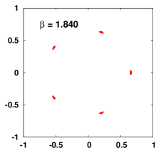
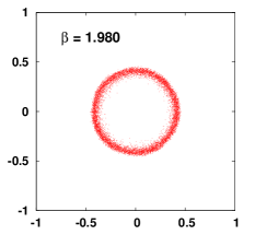
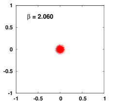
Figure 1: Scatter plot of $M_{L}$ at $\beta$=1.84, 1.98 and 2.06 in $Z(5)$ on a $512^{2}\times 4$ lattice.

A clear indication of the three-phase structure emerges from the inspection of the scatter plot of the complex magnetization $M_{L}$ at different values of $\beta$: as we move from low to high $\beta$, we observe the transition from an ordered phase ($N$ isolated spots) through an intermediate phase (ring distribution) up to the disordered phase (uniform distribution around zero) – see Fig. 1.

The first step is to determine the two critical couplings in the thermodynamic limit, $\beta_{\rm c}^{(1)}$ and $\beta_{\rm c}^{(2)}$, that separate the three phases. To this aim we find the value of $\beta_{c}$ which provides the best overlap of universal observables, plotted for different values of $L$ against $(\beta-\beta_{\rm c}^{(1)})(\ln L)^{1/\nu}$, with $\nu$ fixed at 1/2. As universal observables we used the Binder cumulant $B_{4}^{(M_{R})}$ and the order parameter $m_{\psi}$ for the first phase transition and the Binder cumulant $U_{L}^{(M)}$ for the second phase transition. In Fig. 2 we show as an example the plots of one of these universal observables against $\beta$ and against $(\beta-\beta_{\rm c}^{(1)})(\ln L)^{1/\nu}$, with $\nu$ fixed at 1/2. In Table 1 we report the determinations of the critical couplings $\beta_{\rm c}^{(1)}$ and $\beta_{\rm c}^{(2)}$, in $Z(N)$ with $N$=5, 8, 13 and 20, for $N_{t}$=2, 4, 8 and 12.

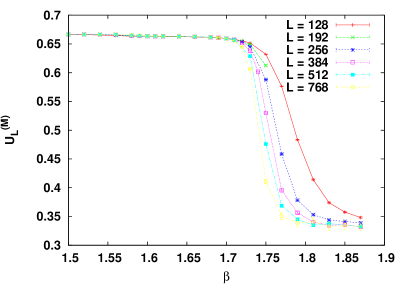
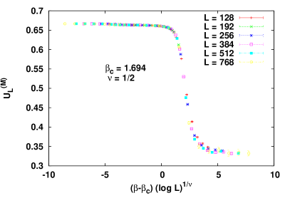
Figure 2: $U_{L}^{(M)}$ as function of $\beta$ (left) and of $(\beta-\beta_{c})(\ln L)^{1/\nu}$ (right) in $Z(5)$ $N_{t}=2$ model.

Table 1: Values of $\beta_{\rm c}^{(1)}$ and $\beta_{\rm c}^{(2)}$ obtained for various $N_{t}$ in $Z(N)$ with $N=5,\ 8,\ 13$ and 20.

$N$	$N_{t}$	$\beta_{\rm c}^{(1)}$	$\beta_{\rm c}^{(2)}$
5	2	1.617(2)	1.694(2)
5	4	1.943(2)	1.990(2)
5	6	2.05(1)	2.08(1)
5	8	2.085(2)	2.117(2)
5	12	2.14(1)	2.16(1)
8	4	2.544(8)	4.688(5)
8	8	3.422(9)	4.973(3)

$N$	$N_{t}$	$\beta_{\rm c}^{(1)}$	$\beta_{\rm c}^{(2)}$
13	2	1.795(4)	9.699(6)
13	4	2.74(5)	11.966(7)
13	8	3.358(7)	12.710(2)
20	4	2.57(1)	28.15(2)
20	8	3.42(5)	29.731(4)

Now, we are able to extract some critical indices and check the hyperscaling relation. Since we are using the observables in the dual model, the transitions change places: the first transition is governed by the behavior of $M_{R}$, the second one by the behavior of $M_{L}$.

We start the discussion from the second transition. According to the standard finite-size scaling (FSS) theory, the equilibrium magnetization $|M_{L}|$ at criticality should obey the relation $|M_{L}|\sim L^{-\beta/\nu}$, if the spatial extension $L$ of the lattice is large enough. Therefore, we fit data of $|M_{L}|$ at $\beta^{(2)}_{\rm c}$, on all lattices with size $L$ not smaller than a given $L_{\rm min}$, with the scaling law $|M_{L}|=AL^{-\beta/\nu}$. The FSS behavior of the susceptibility $\chi^{(M)}_{L}$ is given by $\chi^{(M)}_{L}\sim L^{\gamma/\nu}$, where $\gamma/\nu=2-\eta$ and $\eta$ is the magnetic critical index. Therefore we fit data of $\chi^{(M)}_{L}$ at $\beta^{(2)}_{\rm c}$, on all lattices with size $L$ not smaller than a given $L_{\rm min}$, according to the scaling law $\chi^{(M)}_{L}=AL^{\gamma/\nu}$.

The reference value for the index $\eta$ at this transition is 1/4, whereas the the hyperscaling relation to be fulfilled is $\gamma/\nu+2\beta/\nu=d=2$. We find (see [11, 13] for details) that in most cases the values of $\eta$ and $d$ are close to those predicted by universality. The small discrepancy from the exact values $\eta=0.25$ and $d=2$ may be caused by the asymptotically vanishing parts of the scaling behavior of the observables $|M_{L}|$ and $\chi^{(M)}_{L}$, that we are not taking into account, but may be significant for smaller lattice sizes.

The procedure for the determination of the critical indices at the first transition is similar to the one for the second transition, with the difference that the scaling laws given above are to be applied to the rotated magnetization, $M_{R}$, and to its susceptibility, $\chi_{L}^{(M_{R})}$, respectively.

The reference value for the index $\eta$ at this transition is $4/N^{2}$, i.e. $\eta=0.16$ for $N=5$ and $\eta\approx 0.0237$ for $N=13$, whereas the hyperscaling relation to be fulfilled is $\gamma/\nu+2\beta/\nu=d=2$. Also here we have found (see [11, 13] for details) a general agreement between the $\eta$ and $d$ values obtained and those predicted by universality. However, the expected value of $\beta/\nu$ is very small, ($2/N^{2}$), so other, asymptotically vanishing, terms can have a great impact on its determination on finite-sized lattices. This is especially evident for $Z(13)$ with $N_{t}=4$, where $\beta/\nu$ turned out to be negative indicating that the magnetization $M_{R}$ grows with lattice size.

There is an independent method to determine the critical exponent $\eta$, which does not rely on the prior knowledge of the critical coupling, but is based on the construction of a suitable universal quantity [14, 15]. The idea is to plot $\chi_{L}^{(M_{R})}L^{\eta-2}$ versus $B_{4}^{(M_{R})}$ and to look for the value of $\eta$ which optimizes the overlap of curves from different volumes. This method is illustrated in Fig 3. for $Z(13)$ model with $N_{t}=4$.

Concerning the value of the critical index $\nu$, the methods used in this work do not allow for the direct determination of its value. When locating critical points we have fixed $\nu$ at 1/2. This value appears to be well in agreement with all numerical data.

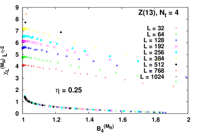
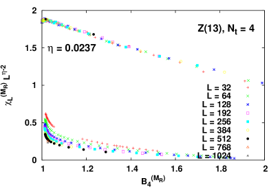
Figure 3: Correlation between $\chi_{L}^{(M_{R})}L^{\eta-2}$ and the Binder cumulant $B_{4}^{(M_{R})}$ in $Z(13)$ with $N_{t}=4$ for $\eta=0.25$ (left) and for $\eta=0.0237$ (right) on lattices with different size.

To provide further evidence on the nature of the phase transitions we have performed Monte Carlo simulation of the original gauge model, in particular we considered the $Z(5)$ LGT with $N_{t}=2,4$ and spatial extent $L\in[64-512]$. The typical statistics was $10^{5}$. In general, error bars are larger and results for critical indices are not so precise as in dual model simulations. Nevertheless, we can state that (i) the critical index $\eta$ is compatible with its $2D$ value; (ii) the values of the indices at two transitions are indeed interchanged as explained before (see [11] for details).

Finally, we have calculated the average action and the specific heat around the transitions in $Z(5)$ LGT with $N_{t}$=2 and $N_{t}=4$. In all cases the dependence of these quantities on $\beta$ turned out to be continuous, thus ruling out first and second order transitions and being compatible with a transition of infinite order (see [11] for details).

4 Conclusions

We have studied $3D$ $Z(N>4)$ vector LGTs at the finite temperature, using the exact dual transformation to generalized $3D$ $Z(N)$ spin models and determined the two critical couplings of $Z(N=5,8,13,20)$ vector LGTs and given estimates of the critical indices $\eta$ at both transitions. We have observed, for the first time in these models, a scenario with three phases: disordered phase at small $\beta$, massless or BKT phase at intermediate values of $\beta$, ordered phase at larger and larger values of $\beta$ as $N$ increases. This matches perfectly with the $N\to\infty$ limit, i.e. the $3D$ $U(1)$ LGT, where the ordered phase is absent.

We have found that the values of the critical index $\eta$ at the two transitions are compatible with the theoretical expectations. The index $\nu$ also appears to be compatible with the value $1/2$, in agreement with universality predictions. We conclude that finite-temperature $3D$ $Z(N>4)$ vector LGTs undergo two phase transitions of the BKT type and belong to the universality class of the $2D$ $Z(N)$ vector models.

References

- [1] D. Horn, M. Weinstein and S. Yankielowicz, Phys. Rev. D 19 (1979) 3715; M.B. Einhorn, R. Savit, and E. Rabinovici, Nucl. Phys. B 170 (1980) 16.
- [2] A. Ukawa, P. Windey, A.H. Guth, Phys. Rev. D 21 (1980) 1013.
- [3] G. Bhanot and M. Creutz, Phys. Rev. D 21 (1980) 2892.
- [4] M. Caselle, M. Hasenbusch, Nucl. Phys. B 470 (1996) 435.
- [5] B. Svetitsky, L. Yaffe, Nucl. Phys. B 210 (1982) 423.
- [6] M. Caselle et al., PoS LAT 2007 (2007) 306 [arXiv:0710.0488 [hep-lat]].
- [7] O. Borisenko et al., Phys. Rev. E 86 (2012) 051131.
- [8] O. Borisenko et al., PoS LATTICE 2012 270 [arXiv:1212.1051 [hep-lat]].
- [9] V.L. Berezinskii, Sov. Phys. JETP 32 (1971) 493; J. Kosterlitz, D. Thouless, J. Phys. C 6 (1973) 1181; J. Kosterlitz, J. Phys. 7 (1974) 1046.
- [10] O. Borisenko, PoS LAT 2007, 170 (2007); O. Borisenko, M. Gravina, A. Papa, J. Stat. Mech. 0808 (2008) P08009; O. Borisenko et al., J. Stat. Mech. 1004 (2010) P04015; O. Borisenko et al., PoS LATTICE 2010 (2010) 274 [arXiv:1101.0512 [hep-lat]]; O. Borisenko et al., PoS LATTICE 2011 (2011) 304 [arXiv:1110.6385 [hep-lat]]; O. Borisenko et al., Phys. Rev. E 85 (2012) 021114.
- [11] O. Borisenko et al., Nucl. Phys. Rev. B 870 (2013) 159.
- [12] S. Elitzur, R.B. Pearson, J. Shigemitsu, Phys. Rev. D 19 (1979) 3698.
- [13] O. Borisenko et al., in preparation.
- [14] D. Loison, J. Phys.: Condens. Matter 11 (1999) L401.
- [15] O. Borisenko et al., Phys. Rev. E 83 (2011) 041120.