Computing Exact Clustering Posteriors
with Subset Convolution

Abstract

An exponential-time exact algorithm is provided for the task of clustering $n$ items of data into $k$ clusters. Instead of seeking one partition, posterior probabilities are computed for summary statistics: the number of clusters, and pairwise co-occurrence. The method is based on subset convolution, and yields the posterior distribution for the number of clusters in $O(n3^{n})$ operations, or $O(n^{3}2^{n})$ using fast subset convolution. Pairwise co-occurrence probabilities are then obtained in $O(n^{3}2^{n})$ operations. This is considerably faster than exhaustive enumeration of all partitions.

1 Introduction

The vast majority of clustering literature is dedicated to finding one particularly good partition, i.e. a definite clustering of the data. In a probabilistic setting, a good partition may be defined as one that has high likelihood, or high posterior probability compared to other partitions that have been considered. However, posterior probabilities are usually known only up to an unknown normalizing constant over the clustering space. Thus, one may deduce that one partition is, say, $10^{20}$ times more probable than another partition, while having no idea whether the posterior probability itself is on the order of $0.5$, or perhaps $10^{-10}$. Clearly, from the perspective of Bayesian inference, this is an unfortunate situation, and it is in general unknown how well standard Monte Carlo sampling strategies (e.g., ?, ?, ?, ?) can approximate the true partition posterior.

Furthermore, even the optimal partition may have a vanishingly tiny posterior probability. For instance, if the clusters are not very clearly distinguishable in the data, the posterior mass may be spread over a large number of partitions. Suppose that the optimal partition has $k=4$ clusters and the posterior probability $10^{-10}$. It appears reasonable to claim that posterior inferences should also be concerned with the remaining posterior mass $1-10^{-10}\approx 1$, and in particular how the probability mass is spread over different values of $k$. In addition, it remains in practice unknown how the posterior distribution over possible data partitions is affected by the dimensionality of observed features, as well as by the choice of a model and prior distribution for model parameters and partitions, due to the rapidly increasing size of the clustering space, which makes full enumeration infeasible in practice.

Since posterior probabilities would be highly desirable for meaningful collections of partitions, we introduce here an approach to their efficient calculation based on subset convolution. In particular, we are interested in posterior probabilities for the following two kinds of propositions: (1) “The data are appropriately represented by $k$ distinct clusters.” (2) “The two items $i$ and $j$ belong to the same cluster” (for each pair $i,j$). We shall show how these probabilities can be exactly evaluated with subset convolution without actually enumerating all partitions. The pairwise co-occurrence probabilities in the latter proposition are also directly useful for deriving a model-averaged estimate of the partition under specific loss-functions and have been considered by multiple authors (e.g., ?, ?, ?, ?, ?).

To demonstrate the use of a subset convolution, we consider a variant of the product partition model, which has been studied, e.g., by ? (?, ?, ?, ?, ?, ?).

A dynamic programming method to find the optimal partition was first suggested by ? (?), and implemented by ? (?). ? (?) proposed various speedups to the original method, but in general the dynamic programming approach has time requirement $O(3^{n})$. In a line of different work, ? (?) showed how dynamic programming can be used to efficiently find the posterior mode partition even for very large sets of items, however, the method is restricted only to the case where sufficient statistics from data are univariate for each cluster. While the goal of searching for optimum is very different from computing the posterior, computationally they involve highly similar steps.

Applications of subset convolution to various combinatorial problems, including partitioning, are described by ? (?) and ? (?). To the best of our knowledge, use of subset convolution to computing posteriors of $k$ and pairwise co-occurrence has not been considered previously.

The remainder of the paper is structured as follows. The main results are derived in the three subsequent sections and some numerical illustrations are given in the penultimate section.The final section concludes with some remarks and discussion about potential generalizations and wider application of the presented ideas.

2 Definitions and preliminaries

Let $U$ denote a set of $n$ elements, or items, labeled by integers $\{1,\ldots,n\}$. Each data item $i$ is associated with some $D$-dimensional feature vector $y_{i}=(y_{i1},\ldots,y_{iD})$, and the whole data set will be denoted by $y$.

A cluster is a subset of $U$. An unordered partition of $U$ is a set of disjoint, nonempty clusters whose union is $U$. An ordered partition is a tuple of disjoint, nonempty clusters whose union is $U$. A partition of cardinality $k$ is called a $k$-partition. In a singleton partition each item forms its own cluster ($k=n$). In a trivial partition all items are clustered together ($k=1$).

The distinction between ordered and unordered partitions is crucial when counting partitions, computing sums, or defining probability distributions over them. The distinction is also at the roots of the so-called label switching problem, discussed e.g. by ? (?). The number of unordered $k$-partitions of $n$ items is the Stirling number of the second kind, denoted $S(n,k)$, while the number of ordered $k$-partitions is $k!\times S(n,k)$. Consider the intuitive notion of “the” singleton partition: it is either unique (unordered) or there are $n!$ of them (ordered). The trivial partition, in contrast, is unique in both cases. In the following, a partition is assumed to be unordered unless otherwise noted.

The task of clustering in general is to characterize particularly good or plausible data partitions in some statistical sense. We adopt here the Bayesian perspective, where the (prior) predictive probability of the data (also termed as evidence) is conditioned on the partition, and seek to characterize posterior probability within the space of possible partitions. This is in general a daunting task since the partition space grows quickly with respect to $n$. For instance, suppose $n=20$, then, the number of 4-partitions alone is $S(20,4)\approx 4.5\times 10^{10}$, and the number of all partitions (for $k=1,\ldots,20$) is the 20th Bell number, about $5.2\times 10^{13}$. A brute force search or summation over them would be a considerable computing task and similarly, any practically obtainable Monte Carlo sample from the posterior will only cover a small fraction of the space.

3 Partition posterior and subset convolution

Our method targets posterior distribution under a product partition model (?, ?, ?, ?, ?), extended to accommodate an arbitrary prior for $k$, the number of clusters. We assume that the prior probability for an ordered $k$-partition $S=(S_{1},\ldots,S_{k})$ factorizes as

$$p(S)=w_{k}\cdot\prod_{j=1}^{k}f_{\text{prior}}(S_{j}),$$

where $f_{\text{prior}}$ is an arbitrary function defined for the nonempty subsets of $U$, and the factors $w_{1},\ldots,w_{n}$ control the marginal prior probability for $k$. Likewise, we assume that partition marginal likelihood (evidence) factorizes as

$$p(y\;|\;S)=\prod_{j=1}^{k}p(y_{(j)}\;|\;S_{j})=\prod_{j=1}^{k}f_{\text{lik}}(S_{j}),$$

where $f_{\text{lik}}$ expresses the marginal likelihood of data $y_{(j)}$ observed in cluster $S_{j}$, and is also an arbitrary function over subsets. We shall later show examples of standard models satisfying these desiderata. However, our approach could also be applied in the case where marginal likelihoods are not analytically available but are replaced with approximations, such as those based on the Laplace method.

For simplicity $f_{\text{prior}}$ and $f_{\text{lik}}$ are combined as a single function $f(X)=f_{\text{prior}}(X)f_{\text{lik}}(X)$. For completeness we define $f(\varnothing)=0$, which rules out empty clusters. This function $f$ and the factors $w_{1},\ldots,w_{n}$ are the input to our clustering model.

The posterior probability of an ordered $k$-partition is now

$$p(S\;|\;y)=\frac{p(S)p(y\;|\;S)}{p(y)}=Z\cdot w_{k}\cdot\prod_{j=1}^{k}f(S_{j}),$$

where $Z=1/p(y)$ is the normalizing constant.

Note that we define the model for ordered partitions for computational convenience. In practice each unordered $k$-partition is represented as $k!$ ordered $k$-partitions due to permutation.

This model accommodates various partition priors. A widely used prior, where all unordered partitions are equiprobable (uniform on partitions), is obtained by setting $f_{\text{prior}}(X)=1$ for all $X\neq\varnothing$, and $w_{k}=1/(k!\cdot B_{n})$, where $B_{n}$ is the $n$th Bell number. Under this prior, the marginal distribution for $k$ is highly nonuniform.

Another prior is uniform on k, where $p(k)=1/n$ for $k=1,\ldots,n$, and partitions of the same cardinality are equiprobable. This prior, obtained by setting $f_{\text{prior}}(X)=1$ and $w_{k}=1/(k!\cdot n\cdot S(n,k))$, is a convenient way of expressing no strong prior belief about $k$. It does not seem widely used, but occurs as a special case of a larger prior family introduced by ? (?). ? (?) prove that this prior cannot be expressed as an ordinary product partition model.

Yet another prior is based on a Dirichlet process (DP) with weight parameter $\theta$ (?, ?, ?). This is obtained by $f_{\text{prior}}(S_{j})=\Gamma(|S_{j}|)$ and $w_{k}=\Gamma(\theta)/(\Gamma(\theta+n)\cdot k!)$.

3.1 Computing posterior of $k$

The posterior probability of $k$ clusters equals under the above formulation

$$p(k\;|\;y)=Z\cdot w_{k}\cdot\sum_{\begin{subarray}{c}S\in{\cal S}\\ |S|=k\end{subarray}}{\prod_{j=1}^{k}}f(S_{j}),$$ (1)

where ${\cal S}$ is the space of ordered partitions. This sum of products is conveniently expressed by means of subset convolution. Given two real-valued functions $f$ and $g$ defined on the subsets of $U$, their subset convolution, or convolution for short, is the function

$$(f*g)(X)=\sum_{A\subseteq X}f(A)\cdot g(X\setminus A),\quad\text{for all $X\subseteq U$},$$ (2)

or equivalently in a more symmetric form,

$$(f*g)(X)=\sum_{\begin{subarray}{c}A,B\subseteq X\\ A+B=X\end{subarray}}f(A)\cdot g(B),$$

where $A+B=X$ represents disjoint union. Convolution is associative, and iterative application yields

$$(f_{1}*\ldots*f_{k})(X)=\sum_{\begin{subarray}{c}A_{1},\ldots,A_{k}\subseteq X\\ A_{1}+\ldots+A_{k}=X\end{subarray}}\prod_{j=1}^{k}f_{j}(A_{j}).$$

In other words, $k$-fold convolution expresses summation over ordered $k$-partitions of a set $X$. Writing (1) in terms of iterated convolution, we arrive at the following proposition.

Proposition 1 (Posterior of $k$)

The posterior probability for the number of clusters being $k$ is

$$p(k\;|\;y)=Z\cdot w_{k}\cdot f^{(k)}(U),$$ (3)

where $f^{(k)}=(f*\ldots*f)$ denotes the convolution of $k$ copies of $f$.

The normalizing constant $Z$ is obtained from the constraint $\sum_{k=1}^{n}p(k\;|\;y)=1$.

For a single set $X$, a direct evaluation of the sum (2) yields the convolution $(f*g)(X)$ in $O(2^{|X|})$ arithmetic operations. Repeating for all $X\subseteq U$ yields the full convolution table for $f*g$ in $O(3^{n})$ operations; we shall call this method the direct subset convolution. Assuming that $f$ has been tabulated for all $2^{n}$ subsets of $U$ (all possible clusters), the tables for $f^{(2)},\ldots,f^{(n)}$ can be computed iteratively with $n-1$ convolutions. Since the exact posterior distribution for $k$ can be computed from the quantities $f(U),f^{(2)}(U),\ldots,f^{(n)}(U)$ using (3), we obtain the following.

Corollary 1

If $f$ has been computed for all $X\subseteq U$, the full posterior distribution for $k$ can be computed in $O(n3^{n})$ arithmetic operations.

For example, for $n=20$ items, the number of operations needed is on the order of $n3^{n}\approx 7\times 10^{10}$, much less than if the $5.2\times 10^{13}$ possible (unordered) partitions were actually enumerated and their posterior probabilities computed one by one.

A further speedup for large $n$ can be achieved by using fast subset convolution, invented by ? (?), which requires $O(n^{2}2^{n})$ operations instead of $O(3^{n})$. However, for moderate values of $n$, such as 20, the savings are not extensive. An additional complication is that fast subset convolution involves both addition and subtraction, potentially leading to large rounding errors in floating point arithmetic. In our experiments, already for $n=18$ rounding errors caused the result from fast subset convolution to be completely erroneous. This can be avoided, with some extra computational cost, by using exact arithmetic with arbitrary-precision integers with a software library such as GMP (?, ?). In comparison, direct subset convolution does not involve subtraction, and in our experiments floating point arithmetic has been sufficiently accurate.

3.2 Computing posterior pairwise co-occurrence

The main goal of clustering is to identify which items belong together and which don’t. By asking this question for all items simultaneously, one is led to seeking a single partition as the candidate for how items should be merged or separated from each other. But in numerous situations the data do not clearly distinguish one partition as the correct one, and many alternative partitions may have considerable posterior mass. For meaningful posterior conclusions the partition probabilities need to be summarized in a sensible manner to provide model-averaged inference.

A natural approach is to consider each pair $i,j$ of items at a time and evaluate the posterior probability of the event $C_{ij}$ that they belong to the same cluster. We shall call this the posterior pairwise co-occurrence (probability). If posterior pairwise co-occurrence is computed for all item pairs, the results can be summarized as a co-occurrence matrix, as suggested by ? (?) and also considered more in detail by ? (?, ?, ?, ?). In particular, it can be shown that an optimal partition estimate can be derived from the co-occurrence matrix under a more natural loss function than the zero-one loss leading to the choice of mode partition (?, ?). In (?, ?), a partition is sought that minimizes expected loss, where loss is defined by the numbers of misassigned item pairs. The expected loss, over the space of partitions, can be directly computed from the co-occurrence matrix, if that is available.

Consider first the joint posterior for $(k,C_{ij})$, i.e. the probability that the data comes from exactly $k$ clusters such that items $i$ and $j$ are in the same cluster. This is obtained by summing the posterior (1) over all ordered $k$-partitions where $C_{ij}$ holds. Now, since under our assumptions likelihood and partition prior are symmetric with respect to cluster indexing, all permutations of an ordered partition have the same probability; in particular, the probability that items $i$ and $j$ are in the same cluster (one of $S_{1},\ldots,S_{k}$) equals $k$ times the probability that they are in the first cluster $S_{1}$. Since $U\setminus S_{1}$ must be covered by the other clusters $S_{2},\ldots,S_{n}$, we have

$$p(k,C_{ij}\;|\;y)=Z\cdot k\cdot w_{k}\cdot\sum_{\begin{subarray}{c}S_{1}\subseteq U\\ i,j\in S_{1}\end{subarray}}f(S_{1})\cdot(f^{(k-1)})(U\setminus S_{1}).$$

Summing over partition cardinalities we obtain the following proposition.

Proposition 2 (Posterior pairwise probability)

The posterior probability for items $i$ and $j$ being in the same cluster equals

$$p(C_{ij}\;|\;y)=Z\cdot\sum_{k=1}^{n}\left(k\cdot w_{k}\cdot\sum_{\begin{subarray}{c}S_{1}\subseteq U\\ i,j\in S_{1}\end{subarray}}f(S_{1})\cdot(f^{(k-1)})(U\setminus S_{1})\right).$$ (4)

The inner sum in (4) has $2^{n-2}$ terms. Repeating for all pairs $i,j$ we have the following:

Corollary 2

If the iterated convolutions $f^{(2)},\ldots,f^{(n-1)}$ have been computed, the full posterior co-occurrence matrix can be computed in $O(n^{3}2^{n})$ arithmetic operations.

3.3 Finding the mode partition

Although our emphasis lies in posterior summary statistics over partitions, it is worth noting that a slight variant of subset convolution can be used for finding the mode partition. If the summation in (1) is replaced with maximization, one obtains the maximum posterior probability among $k$-partitions. Now this can be computed using a variant of subset convolution, where the summation is replaced with maximization (i.e., the subset convolution is performed over the max-product semiring, instead of the usual sum-product ring). This yields an $O(n3^{n})$ algorithm for finding the maximum-probability $k$-partitions for $k=1,\ldots,n$. The maximum among those is of course the global mode partition. In fact, this method is equivalent to Jensen’s dynamic programming algorithm (?, ?), now expressed in terms of subset convolution.

4 Examples of data models

Our method takes as its input a table of the function $f(X)$ for all $2^{n}-1$ nonempty subsets of $U$. Thus no restrictions are placed on the form of the likelihood function, as long as it can be feasibly computed for $2^{n}-1$ sets. We have experimented with two models where the marginal likelihood is analytically available. It should be noted that the general method of subset convolution is not limited to these two models. For example, for discrete data the beta-binomial model generalizes in a straightforward fashion to a Dirichlet-multinomial or gamma-Poisson family of distributions.

4.1 Beta-binomial model for binary data

For binary data we assume a Bernoulli distribution with a beta prior (?, ?, pp. 157, 160). For each cluster $S_{j}$ and feature $d$, independently from other clusters and features, we assume an unknown parameter $m_{jd}$ (cluster mean) such that

$$m_{jd} \sim\operatorname{Beta}(\alpha,\beta)$$

$$(y_{id}\;|\;m_{jd}) \sim\operatorname{Bernoulli}(m_{jd}),\quad\text{for items $i\in S_{j}$},$$

where $\alpha,\beta$ are prior hyperparameters. This implies that within a cluster and a variable, the counts of zeros and ones are binomially distributed, conditional on $m_{jd}$. The marginal likelihood for the data $y_{(j)d}$ observed in cluster $S_{j}$ for feature $d$ can be expressed in terms of the sufficient statistics $(c,s)$, where $c=|S_{j}|$ is cluster size (number of items), and $s=\sum_{i\in S_{j}}y_{ji}$ is the number of observed ones. Integrating out the binomial parameters, we obtain the marginal likelihood

$$p(y_{(j)d})=\frac{\Gamma(\alpha+s)\Gamma(\beta+c-s)\Gamma(\alpha+\beta)}{\Gamma(\alpha+\beta+c)\Gamma(\alpha)\Gamma(\beta)}.$$

4.2 Gamma-normal model for continuous data

For continuous data we assume normal distribution with a normal-gamma prior, as described by, e.g., ? (?, pp. 168–171) and ? (?, p. 440). For each cluster $S_{j}$ and feature $d$, we assume two unknown parameters $m_{jd}$ (cluster mean) and $r_{jd}$ (cluster precision) such that

$$r_{jd} \sim\operatorname{Gamma}(\alpha,\beta)$$

$$(m_{jd}\;|\;r_{jd}) \sim N(\mu,1/(\tau r_{jd}))$$

$$(y_{id}\;|\;m_{jd},r_{jd}) \sim N(m_{jd},1/r_{jd}),\quad\text{for items $i\in S_{j}$},$$

where $\alpha,\beta,\mu,\tau$ are prior hyperparameters. The marginal likelihood can be expressed in terms of the sufficient statistics $(c,s,q)$, where $c=|S_{j}|$ is cluster size, $s=\sum_{i\in S_{j}}y_{ji}$ is the sum of data, and $q=\sum_{i\in S_{j}}y_{ji}^{2}$ is the sum of squared data. The marginal likelihood is derived e.g. by ? (?), and in our notation it becomes

$$p(y_{(j)d})=\frac{\Gamma(\alpha_{c})}{\Gamma(\alpha)}\frac{\beta^{\alpha}}{\beta_{c}^{\alpha_{c}}}\left(\frac{\tau}{\tau_{c}}\right)^{1/2}(2\pi)^{-c/2},$$

where

$$\alpha_{c} =\alpha+c/2,$$

$$\beta_{c} =\beta+\frac{q-s^{2}/c}{2}+\frac{\tau(s-c\mu)^{2}/c}{2(\tau+c)},$$

$$\tau_{c} =\tau+c.$$

5 Experiments

5.1 Clustering posteriors with a continuous model

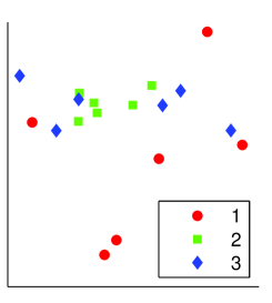
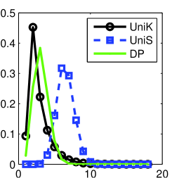
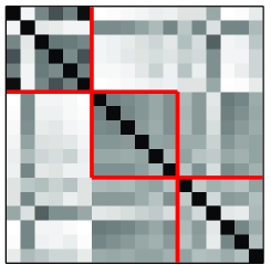
Figure 1: Simulated normal data, $k=3$, $n=18$, $D=2$. Left: original data. Center: Posterior distribution for $k$ with three priors (uniform on $k$, uniform on partitions, and DP with $\theta=1$). Right: Posterior pairwise co-occurrence matrix (dark indicates high probability; red lines highlight the generating clusters).

For a simple illustration, let us consider $18$ items generated from $3$ clusters of 6 items each, with bivariate normal data, where the cluster parameters $(m_{jd},r_{jd})$ were randomly generated with hyperparameters $\alpha=1$, $\beta=1$, $\mu=0$, $\tau=1$. The data are shown in Figure 1 (left), colored by the true (generating) partition.

Assuming the hyperparameters known, but partition unknown, the posteriors for $k$ and pairwise co-occurrence were computed using subset convolution. Assuming uniform prior on $k$, the posterior (Figure 1 center, black line) is peaked at $k=2$, which seems reasonable by visual inspection of the data, as the clusters 2 and 3 overlap considerably. The posterior distribution shows the inherent uncertainty over $k$; computing just the mode partition would not provide such information.

With a DP prior ($\theta=1$), the posterior is similar, but peaked at $k=3$; note that the prior is itself peaked at $k=3$, and in general favors partitions of small cardinality.

If all unordered partitions are assumed a priori equiprobable, the posterior (Figure 1 center, blue line) is peaked at $k=6$. This undesirable behavior is due to the strong prior preference for large partitions, simply because there are so many of them. For example, there are $S(18,3)\approx 6.4\times 10^{7}$ unordered $3$-partitions, but $S(18,6)\approx 1.1\times 10^{11}$ unordered $6$-partitions. Assuming them equiprobable implies a prior belief that $k=6$ is about $1700$ times more probable than $k=3$.

The matrix of posterior pairwise co-occurrence probabilities (assuming uniform prior on $k$) is shown in Figure 1 (right). The items are ordered according to the generating partition for visual inspection. The first cluster stands clearly apart (with the exception of the second item, which is the red dot on the far left).

We also computed the optimal partitions for $k=1,\ldots,n$ using the method described in subsection 3.3, again assuming uniform prior on $k$. The global mode turns out to be the trivial partition with posterior probability $0.094$. For $k=2,3$ the optimal partitions have much lower posterior probabilities $0.014$ and $0.001$, respectively. It is apparent that the mode partition in itself is not well representative of the full posterior distribution.

The computation of the full posterior for $k$ and pairwise co-occurrence takes about 7 minutes of CPU time on a 2.4 GHz AMD Opteron, using a C implementation of direct subset convolution. We estimate that full enumeration of all unordered partitions would have taken about 64 hours.

5.2 Clustering posteriors with a binary model

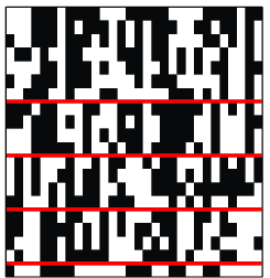
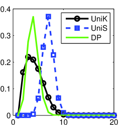
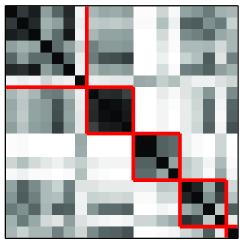
Figure 2: Simulated binary data, $k=5$, $n=20$, $D=30$. Left: original data (red lines indicate cluster boundaries). Center: Posterior distribution for $k$ with three priors (uniform on $k$, uniform on partitions, and DP with $\theta=1$). Right: Posterior pairwise co-occurrence matrix (dark indicates high probability; red lines highlight the generating clusters.

Figure 2 illustrates an experiment with simulated data from five clusters, with 20 items and 30 binary features. The generating partition is a randomly chosen 5-partition and the data were generated with hyperparameters $\alpha=\beta=1$.

The posterior distributions for $k$ (Figure 2 center) and for pairwise co-occurrence (Figure 2 right) show the inherent uncertainty over the correct partition. Yet they also indicate summary statistics that can be reasonably estimated. For example, the pairwise matrix indicates that the four items 8–11 probably belong together (which is correct according to the generating model); likewise for items 12–15.

The mode partition has $k=2$ and posterior probability $0.0267$. For $k=3,4,5$ the optimal partitions have probabilities $0.0050$, $0.0026$ and $0.0005$, respectively. Judging from these posterior probabilities alone — especially if they were unnormalized, and only their ratios could be seen — one might deduce that $k=2$ is an overwhelmingly good model for the data, and that $k=5$ is quite unlikely. Yet the summary statistics lend considerable support to the possibility that $k=5$ (which corresponds to the generating model). Again we must note that posterior probabilities of single partitions do not well represent the full posterior distribution.

The shown posterior distributions are exact, and all uncertainty is due to the data and the probability model assumed; not due to any computational approximation. If the data were more informative, the posterior distributions would correspondingly be more peaked. Here computing the posteriors for $n=20$ took about 3 hours of CPU time whereas a full enumeration of the partitions would take approximately 200 days.

6 Discussion

The convolution approach introduced here has potential for multiple purposes in cluster analysis. For instance, by enabling an exact evaluation of the posterior over the number of clusters and pairwise co-occurrence probabilities, one can investigate how the dimensionality of the feature space and choices of prior hyperparameters affect the power to detect clusters in a particular modeling scenario. Another application is to use the exact posterior in a proposal operator for an Markov chain Monte Carlo sampling algorithm. Obviously, the exponential time requirement limits the applicability of the method to fairly modest instances, on the order of 20–25 items. Even so, we think that having an exact posterior at least in such cases can serve as a useful “gold standard” when evaluating the performance and the characteristics of other, more practical methods. Furthermore, the exact posteriors could be used for larger data sets by segmenting the data into several small subsets and evaluating the posteriors separately for each of them. It appears as an attractive target for further research to investigate intelligent strategies for combining posterior information from the different segments and then proceeding towards global partition inferences.

Acknowledgments

This research was funded by the ERC grant no. 239784 and AoF grant no. 251170.

References

- Barry HartiganBarry Hartigan Barry, D., Hartigan, J. (1992). Product partition models for change point problems. The Annals of Statistics, 20(1), 260–279.
- Bernardo SmithBernardo Smith Bernardo, J. M., Smith, A. F. M. (1994). Bayesian theory. John Wiley and Sons.
- Björklund, Husfeldt, Kaski, KoivistoBjörklund et al. Björklund, A., Husfeldt, T., Kaski, P., Koivisto, M. (2007). Fourier meets Möbius: fast subset convolution. In Proceedings of the thirty-ninth annual ACM symposium on Theory of computing (STOC 07) (pp. 67–74).
- Corander, Gyllenberg, KoskiCorander et al. Corander, J., Gyllenberg, M., Koski, T. (2009). Bayesian unsupervised classification framework based on stochastic partitions of data and a parallel search strategy. Advances in Data Analysis and Classification, 3(1), 3–24.
- DahlDahl Dahl, D. (2009). Modal clustering in a class of product partition models. Bayesian Analysis, 4(2), 243–264.
- Dawson BelkhirDawson Belkhir Dawson, K. J., Belkhir, K. (2001). A Bayesian approach to the identification of panmictic populations and the assignment of individuals. Genetics Research, 78(1), 59–77.
- DeGrootDeGroot DeGroot, M. H. (1970). Optimal statistical decisions. McGraw-Hill.
- Fomin KratschFomin Kratsch Fomin, F., Kratsch, D. (2010). Exact exponential algorithms. Springer-Verlag.
- GMPGMP GMP – The GNU multiple precision arithmetic library. (n.d.). http://gmplib.org/.
- HartiganHartigan Hartigan, J. (1990). Partition models. Communications in Statistics – Theory and Methods, 19(8), 2745–2756.
- Hubert, Arabie, MeulmanHubert et al. Hubert, L. J., Arabie, P., Meulman, J. J. (2001). Combinatorial data analysis: Optimization by dynamic programming. SIAM.
- Huelsenbeck AndolfattoHuelsenbeck Andolfatto Huelsenbeck, J. P., Andolfatto, P. (2007). Inference of population structure under a Dirichlet process model. Genetics, 175(4), 1787–1802.
- Jain NealJain Neal Jain, S., Neal, R. (2004). A split-merge Markov chain Monte Carlo procedure for the Dirichlet process mixture model. Journal of Computational and Graphical Statistics, 13(1), 158–182.
- JensenJensen Jensen, R. E. (1969). A dynamic programming algorithm for cluster analysis. Journal of the Operations Research Society of America, 17(6), 1034–1057.
- Knorr-Held RaßerKnorr-Held Raßer Knorr-Held, L., Raßer, G. (2000). Bayesian detection of clusters and discontinuities in disease maps. Biometrics, 56(1), 13–21.
- Lau GreenLau Green Lau, J. W., Green, P. J. (2007). Bayesian model-based clustering procedures. Journal of Computational and Graphical Statistics, 16, 526–558.
- MurphyMurphy Murphy, K. P. (2007). Conjugate Bayesian analysis of the Gaussian distribution (Tech. Rep.). (Available at http://www.cs.ubc.ca/~murphyk/Papers/bayesGauss.pdf)
- NealNeal Neal, R. (2000). Markov chain sampling methods for Dirichlet process mixture models. Journal of Computational and Graphical Statistics, 9(2), 249–265.
- O’HaganO’Hagan O’Hagan, A. (1997). Contribution to discussion of ’On Bayesian analysis of mixtures with an unknown number of components’ by S. Richardson and P. J. Green. Journal of the Royal Statistical Society B, 59(4), 772.
- Quintana IglesiasQuintana Iglesias Quintana, F. A., Iglesias, P. L. (2003). Bayesian clustering and product partition models. Journal of the Royal Statistical Society B, 65(2), 557–574.
- StephensStephens Stephens, M. (2000). Dealing with label switching in mixture models. Journal of the Royal Statistical Society B, 62(4), 795–809.
- van Os Meulmanvan Os Meulman van Os, B. J., Meulman, J. J. (2004). Improving dynamic programming strategies for partitioning. Journal of Classification, 21(2), 207–230.