Universal features of dynamic heterogeneity in supercooled liquids

Abstract

A few years ago it was showed that some systems that have very similar local structure, as quantified by the pair correlation function, exhibit vastly different slowing down upon supercooling [L. Berthier and G. Tarjus, Phys. Rev. Lett. 103, 170601 (2009); U.R. Pedersen, T.B. Schrøder and J.C. Dyre, Phys. Rev. Lett. 105, 157801 (2010)]. Recently, a more subtle structural quantity, the so-called “point-to-set” length, was found to reliably correlate with the average dynamics [G.M. Hocky, T.E. Markland and D.R. Reichman, Phys. Rev. Lett. 108, 225506 (2012)]. Here we use computer simulations to examine the behavior of fluctuations around the average dynamics, i.e., dynamic heterogeneity. We study five model glass-forming liquids: three model liquids used in previous works and two additional model liquids with finite range interactions. Some of these systems have very similar local structure but vastly different dynamics. We show that for all these systems the spatial extent and the anisotropy of dynamic heterogeneity correlate very well with the average dynamics.

Upon supercooling, universal phenomena are observed in seemingly unrelated glass-forming systems. Similarly, glass transition theories predict universal relationships between different static and dynamic quantities. Some of the relationships predicted by the theories are difficult to verify experimentally but they can be tested in computer simulations. These tests can help to differentiate between different theories. Due to the large computational resources required, simulations often examine one relatively simple model system. However, this does not establish that the relationships between different static or dynamic quantities are truly universal. Here, we examine universal features of dynamic heterogeneity, i.e., fluctuations around the average dynamics.

Our study is inspired by a re-evaluation of the standard van der Waals picture CWA1983 of the liquid state in the context of supercooled liquids’ dynamics. Within the standard picture, the liquid’s local structure, as quantified by the pair correlation function, is primarily determined by the repulsive part of the interparticle potential. Importantly, it was believed (admittedly, with somewhat limited simulational KushickBerne1973 ; YoungAndersen2005 and theoretical Bembenek2000 support) that the local structure, and thus the repulsive part of the potential, also determines the liquid’s dynamics. Therefore, it was surprising when Berthier and Tarjus Berthier2009 showed that two standard model liquids, which differ only by the presence of the attractive part of the potential and have very similar local structure, exhibit vastly different viscous slowing down upon approaching the glass transition. Shortly after this work, Pedersen et al.  Pedersen2010 complicated the picture by finding a system with a purely repulsive potential, the same local structure, and the same dynamics as the model liquid with both repulsive and attractive interactions.

More recently, Hocky et al. Hocky2012 investigated a different, more subtle, static quantity, the so-called “point-to-set” length scale BouchaudBiroli2004 in the systems considered by Berthier and Tarjus, and Pedersen et al. Hocky et al. found that the point-to-set length can have different values for systems with very similar local structure, but it correlates very well with the average dynamics and shows universal features for all the systems studied.

We present results of an extensive computer simulation study that tests the universality of fluctuations around the average dynamics, i.e., dynamic heterogeneity. First, we investigate two standard quantities used to characterize dynamic heterogeneity, the four-point susceptibility, which measures the overall strength of the heterogeneity, and the dynamic correlation length, which measures the spatial extent of the heterogeneity. In addition, we calculate quantities that are sensitive to the anisotropy of dynamic heterogeneity. Investigation of the latter quantities has been prompted by recent experiments of Zhang et al. Zhang2011 , who studied two glassy colloidal systems that differed by the presence of an attractive part of the effective colloid-colloid potential. They found profound dependence of the shape of the clusters of fast particles on the presence of the attractions.

For large enough supercooling, we find that all quantitative characteristics of dynamic heterogeneity for all systems investigated have the same dependence on the relaxation time that characterizes the average dynamics.

We divide the systems we studied into two groups. The systems in the first group (which were also studied by Hocky et al.) are derived from the Kob-Andersen binary Lennard-Jones mixture Kob1994 ; Kob1995a ; Kob1995b . We simulated the standard Kob-Andersen mixture (KA), the Weeks-Chandler-Andersen (WCA) truncation Weeks1971 ; Chandler1983 of the standard mixture, and a system with an inverse power law (IPL) potential that was designed by Pedersen et al. Pedersen2010 . All three systems have similar pair-correlation functions at the same temperature. However, only the KA and IPL mixtures exhibit the same temperature dependence of the relaxation time Berthier2009 ; Pedersen2010 . We studied dynamic properties of these systems as a function of temperature at a fixed volume using Newtonian dynamics.

The second group consists of two 50:50 mixtures of spherical particles with the same size ratio. The first system is a hard sphere (HARD) system, where the particle positions are updated using Monte-Carlo dynamics with local moves Flenner2011 ; Berthier2007 . The second system is a repulsive harmonic sphere (HARM) system BerthierWitten2009 . The HARM system was studied using Newtonian and Brownian dynamics. The control parameter for the hard sphere system is the volume fraction, while it is the temperature for the harmonic spheres.

The details of the simulations and the reduced units which we use to present our results are given in the Supplemental Material supplement .

To find a correlation between dynamic heterogeneity and the average dynamics in systems with different potentials, different control parameters and different underlying microscopic dynamics we need to define a rescaled relaxation time. To this end we use a hallmark property of supercooled liquids: violation of the Stokes-Einstein relation. In the normal liquid state the Stokes-Einstein relation holds and the self-diffusion coefficient is inversely proportional to the relaxation time, $D\sim\tau_{\alpha}^{-1}$. The violation of this relation in supercooled liquids is frequently associated with the appearance of dynamic heterogeneity BerthierDH ; Ediger2000 . We define a rescaled relaxation time in such a way that all systems we study deviate from the Stokes-Einstein relation at the same rescaled relaxation time.

We calculate the self-diffusion coefficient $D$ from the mean-square-displacement, $D=\lim_{t\rightarrow\infty}(6tN)^{-1}\left<\sum_{n}|\mathbf{r}_{n}(t)-\mathbf{r}_{n}(0)|^{2}\right>$. We define the alpha relaxation time $\tau_{\alpha}$ in terms of the self-intermediate scattering function $F_{s}(k;t)$ using the standard relation $F_{s}(k_{0};\tau_{\alpha})=e^{-1}$, where $k_{0}$ is chosen to be around the first peak of the static structure factor $S(k)$. For the KA, WCA, and IPL systems $k_{0}=7.2$, and for the HARM and HARD systems $k_{0}=6.1$.

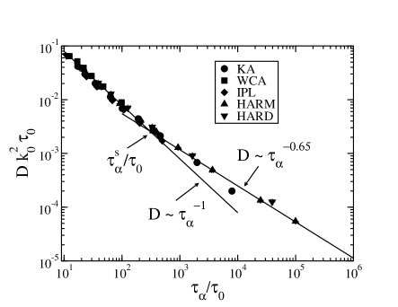
Figure 1: Rescaled self-diffusion coefficient $Dk_{0}^{2}\tau_{0}$ plotted versus rescaled relaxation time $\tau_{\alpha}/\tau_{0}$ for all the systems investigated. The lines are fits of the HARM data to $D\sim\tau_{\alpha}^{-1}$ for $T\geq 12$ and to a fractional Stokes Einstein relation $D\sim\tau_{\alpha}^{-\lambda}$ for $T\leq 7$. The rescaled relaxation time $\tau_{\alpha}^{s}/\tau_{0}$ is when these two fits are equal.

To find the rescaling of the relaxation time, we used the HARM system as a reference. For the remaining systems, we rescaled the relaxation time $\tau_{\alpha}$ by a constant $\tau_{0}$ so that these systems deviate from the Stokes-Einstein relation at the same $\tau_{\alpha}/\tau_{0}$. This procedure results in $\tau_{0}\approx 1/15$ for the KA, WCA, and IPL systems, and $\tau_{0}\approx 70$ for the hard-sphere system. Somewhat unexpectedly, we found that by plotting $Dk_{0}^{2}\tau_{0}$ as a function of $\tau_{\alpha}/\tau_{0}$ we obtain a reasonable collapse of all the data, see Fig. 1.

We note that a crossover time scale (defined by crossing point of two power-law relations showed in Fig. 1) is equal to $\tau_{\alpha}^{s}=303\tau_{0}$. This time scale corresponds to a temperature $T_{s}$ (or volume fraction $\phi_{s}$) located between the onset of glassy dynamics and the mode-coupling transition temperature (see Supplemental Material supplement for more details).

To obtain the four-point susceptibility and the dynamic correlation length we start with an often studied four-point structure factor defined in terms of overlap functions pertaining to individual particles,

$$S_{4}^{\mathrm{ov}}(q;t)=\frac{1}{N}\left<\sum_{n,m}w_{n}(a;t)w_{m}(a;t)e^{i\mathbf{q}\cdot[\mathbf{r}_{n}(0)-\mathbf{r}_{m}(0)]}\right>.$$ (1)

Here $w_{n}(a;t)$ is the overlap function, $w_{n}(a;t)=\Theta[a-|\mathbf{r}_{n}(t)-\mathbf{r}_{n}(0)|]$, where $\Theta(x)$ is Heaviside’s step function. $S_{4}^{\mathrm{ov}}(q;t)$ is the structure factor of the particles that move less than a distance $a$ over a time $t$, and it is used to characterize the size of clusters of slow particles. We calculate this structure factor at time $\tau_{\alpha}^{\mathrm{ov}}$, which is defined in terms of the average overlap function $F_{s}^{\mathrm{ov}}(\tau_{\alpha}^{\mathrm{ov}})=N^{-1}\left<\sum_{N}w_{n}(a;\tau_{\alpha}^{\mathrm{ov}})\right>=e^{-1}$. We choose $a$ such that $\tau_{\alpha}^{\mathrm{ov}}$ is close to the relaxation time $\tau_{\alpha}$ defined in terms of the self-intermediate scattering function. For the KA, WCA, and IPL systems $a=0.25$ and for the HARM and HARD systems $a=0.3$ (note that these choices make the product $k_{0}a$ approximately the same for all systems investigated). We use the previously described procedure Flenner2010 ; Flenner2011 to calculate the four-point susceptibility $\chi^{\mathrm{ov}}_{4}$ and the dynamic correlation length $\xi_{4}^{\mathrm{ov}}$.

First, we investigate the relationship between these two quantities. In Fig. 2 we show $\chi_{4}^{\mathrm{ov}}/K$ plotted versus $\xi_{4}^{\mathrm{ov}}$. Here $K$ is a system dependent scaling constant. We found that $K$ is the same for the KA, WCA, and IPL systems. For $\xi_{4}^{\mathrm{ov}}>2.6$ we find that $\chi_{4}^{\mathrm{ov}}$ grows as $(\xi_{4}^{\mathrm{ov}})^{3}$ for all systems investigated. We note that $\xi_{4}^{\mathrm{ov}}=2.6$ when the system’s relaxation time is $\tau_{\alpha}^{s}$, Fig. 3. We recall that the Random-First-Order Theory (RFOT) approach predicts compact dynamically correlated regions for temperatures below the mode-coupling transition temperature Stevenson2006 . We find $\chi_{4}^{\mathrm{ov}}\propto(\xi_{4}^{\mathrm{ov}})^{3}$, which indicates compact clusters of slow particles, starting from the crossover temperature $T_{s}$ (or volume fraction $\phi_{s}$).

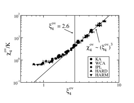
Figure 2: A rescaled dynamic susceptibility $\chi_{4}^{\mathrm{ov}}/K$ versus $\xi_{4}^{\mathrm{ov}}$. Here $K$ is a system dependent scaling constant. $K$ is the same for the KA, WCA, and IPL systems.

We now examine the correlation between the dynamic correlation length $\xi_{4}^{\mathrm{ov}}$ calculated at $\tau_{\alpha}^{\mathrm{ov}}$ and $\tau_{\alpha}^{\mathrm{ov}}/\tau_{0}$. Note that to define a rescaled time scale we use the values of $\tau_{0}$ which were determined before by analyzing the relation between $D$ and $\tau_{\alpha}$. This is justified since the temperature (or volume fraction) dependence of $\tau_{\alpha}^{\mathrm{ov}}$ and $\tau_{\alpha}$ is very similar. We note that the results for all systems investigated collapse onto the same curve when plotted as $\xi_{4}^{\mathrm{ov}}$ versus $\tau_{\alpha}^{\mathrm{ov}}/\tau_{0}$, Fig. 3. While we anticipated having to rescale $\xi_{4}^{\mathrm{ov}}$, this does not seem necessary for the systems studied. We conclude that the spatial extent of dynamic heterogeneity correlates very well with the average dynamics when the average dynamics is rescaled relative to the point at which the Stokes-Einstein relation is violated.

We compare our results to three theoretical scenarios. The relationships between the dynamic correlation length and the relaxation time obtained from these scenarios are showed as lines in Fig. 3. We find that a power law relationship between $\xi_{4}^{\mathrm{ov}}$ and $\tau_{\alpha}^{\mathrm{ov}}$ (dash-dotted line) obtained from a mode-coupling-like approach Biroli2004 ; Biroli2006 ; Szamel2008 is a poor description of the data for more than about a decade of slowing down. Next, we find that a logarithmic relationship $\xi_{4}^{\mathrm{ov}}\sim\ln(\tau_{\alpha}^{\mathrm{ov}})^{1/\zeta}$, inspired by an Adam-Gibbs like Adam1965 or a Random-First-Order Transition (RFOT) theory Kirkpatrick1989 ; Lubchenko2007 , describes well the initial slowing down with $\zeta=1$ (dotted line) but at longer relaxation times $\zeta=2/3$ (dashed line) provides a better fit. Finally, the relation inspired by the facilitation picture, $\ln(\xi_{4})=A\sqrt{\ln(B\tau_{\alpha}^{\mathrm{ov}}/\tau_{0})}+C$ (solid line) Keys2011 , is also compatible with the data. In principle, a more detailed analysis of the existing data (including independent estimates of various theoretical parameters) may be able to distinguish between the latter two approaches. We note, however, that the theoretical scenarios are nearly indistinguishable over a large range of $\xi_{4}$ versus $\tau_{\alpha}^{\mathrm{ov}}/\tau_{0}$. The most direct comparison would be enabled by extending the range of the available (rescaled) relaxation times by some two orders of magnitude.

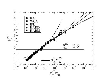
Figure 3: The four-point correlation length $\xi_{4}^{\mathrm{ov}}$ versus the rescaled relaxation time $\tau_{\alpha}^{\mathrm{ov}}/\tau_{0}$. The lines are fits to different theoretical functions. The dash-dotted line is a mode-coupling-like fit $\xi_{4}^{\mathrm{ov}}\sim(\tau_{\alpha}^{\mathrm{ov}})^{1/z}$ where $z=4.8$. The next two fits are inspired by RFOT theory. The dotted line is a fit to $\xi_{4}^{\mathrm{ov}}\sim\ln(\tau_{\alpha}^{\mathrm{ov}})$. For longer relaxation times the data are better described by $\xi_{4}^{\mathrm{ov}}\sim\ln(\tau_{\alpha}^{\mathrm{ov}})^{3/2}$ which is showed as the dashed line. The solid line is a fit to the facilitation prediction of $\ln(\xi_{4}^{\mathrm{ov}})=A\sqrt{\ln(B\tau_{\alpha}^{\mathrm{ov}})}+C$. We also indicated the relaxation time where Stokes-Einstein violation begins (solid vertical line), $\tau_{\alpha}^{s}$, and the correlation length where the relationship $\chi_{4}^{\mathrm{ov}}\sim(\xi_{4}^{\mathrm{ov}})^{3}$ begins (solid horizontal line).

Fig. 2 indicates a change in the spatial organization of dynamic heterogeneity. This fact, together with experimental finding of Zhang et al. Zhang2011 , prompted us to examine in some detail the shape of dynamic heterogeneity. To this end we study a four-point structure factor defined in terms of microscopic self-intermediate scattering functions pertaining to different particles,

$$S_{4}(\mathbf{k},\mathbf{q};t)=\frac{1}{N}\left<\sum_{n,m}\hat{F}_{n}(\mathbf{k};t)\hat{F}_{m}(\mathbf{k};t)e^{i\mathbf{q}\cdot[\mathbf{r}_{n}(0)-\mathbf{r}_{m}(0)]}\right>.$$ (2)

Here $\hat{F}_{n}(\mathbf{k},t)$ is the microscopic self-intermediate scattering function, $\hat{F}_{n}(\mathbf{k},t)=\cos[\mathbf{k}\cdot(\mathbf{r}_{n}(t)-\mathbf{r}_{n}(0))]$. Its ensemble average is the self-intermediate scattering function $F_{s}(k;t)$. A similar four-point structure factor was examined in Ref. Flenner2007 .

The four-point structure factor $S_{4}(\mathbf{k},\mathbf{q};t)$ is sensitive to dynamics along the wave-vector $\mathbf{k}$. A slow spatial decay of correlations of the dynamics along $\mathbf{k}$ would be revealed in the small $q$ values of $S_{4}(\mathbf{k},\mathbf{q};t)$. The spatial decay of correlations of the dynamics along the direction of the initial separation vector $\Delta\mathbf{r}_{nm}(0)=\mathbf{r}_{n}(0)-\mathbf{r}_{m}(0)$ are measured by examination of $S_{4}(\mathbf{k},\mathbf{q};t)$ where $\mathbf{k}$ and $\mathbf{q}$ are parallel, and correlations of the dynamics along a direction perpendicular to $\Delta\mathbf{r}_{nm}(0)$ are measured by examination of $S_{4}(\mathbf{k},\mathbf{q};t)$ when $\mathbf{k}$ and $\mathbf{q}$ are perpendicular. We calculate $S_{4}(\mathbf{k},\mathbf{q};t)$ at a fixed angle $\theta$ between $\mathbf{k}$ and $\mathbf{q}$. We determine $\xi_{4}^{\theta}$ by fitting $S_{4}(\mathbf{k},\mathbf{q};t)$ using the same procedure described in Refs. Flenner2010 ; Flenner2011 ; Flenner2013 .

Shown in Fig. 4 is $\xi_{4}^{\theta}$ for $\theta=0$ and $\theta=\pi/2$ as a function of $\tau_{\alpha}/\tau_{0}$ comment2 . The results for all the systems follow the same trend. For the first 1.5 decades of slowing down correlations along the particles separation vector grows faster than correlations perpendicular to the separation vector, and there is a small dynamics dependence in the growth of $\xi_{4}^{\theta}$, but there is no dependence on the specifics of the interactions for this set of binary glass-formers. The similarity between the KA, WCA, and IPL systems indicates that there is no change in the shape of dynamically heterogeneous regions due to the presence of attractive interactions for this range of relaxation times. This is qualitatively different from the results of Zhang et al. Zhang2011 . We note that in the latter study clusters of fast particles were monitored whereas we examine correlations of slow particles. In addition, Zhang et al. examined dynamics in colloidal glasses whereas we study equilibrium liquids approaching the glass transition.

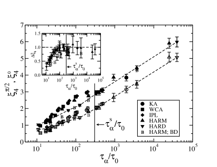
Figure 4: The dynamic correlation length $\xi_{4}^{0}$ and $\xi_{4}^{\pi/2}$ as a function of the rescaled relaxation time $\tau_{\alpha}/\tau_{0}$. The dashed lines connect the data for the hard-sphere system. The points for the HARM system with Brownian dynamics are marked with a $B$, and the error bars, which are about the size of the points, are omitted for clarity. The inset shows the difference $\Delta\xi_{4}=\xi_{4}^{0}-\xi_{4}^{\pi/2}$ as a function of the rescaled relaxation time $\tau_{\alpha}/\tau_{0}$. The horizontal dashed line is $\Delta\xi_{4}=1.0$.

We observe that for all systems the initial growth of $\xi_{4}^{0}$ is faster than the initial growth of $\xi_{4}^{\pi/2}$, see inset to Fig. 4 where we show $\Delta\xi_{4}=\xi_{4}^{0}-\xi_{4}^{\pi/2}$. The correlation length $\xi_{4}^{0}$ grows faster than $\xi_{4}^{\pi/2}$ until the difference between the two is around one particle diameter, then they grow at statistically the same rate as a function of the rescaled relaxation time. The initial growth of $\Delta\xi_{4}$ depends slightly on the microscopic dynamics, but is independent of system. For times exceeding $\tau_{\alpha}^{s}$, $\Delta\xi_{4}$ is around one particle diameter and it is independent of the dynamics or the details of the interactions.

Having a larger $\xi_{4}^{0}$ than $\xi_{4}^{\pi/2}$ is suggestive of the string-like motion reported in previous work Donati1998 ; Kim2000 . However, our work examines the slow particles, while the string-like motion is observed for the fast particles. We leave a more detailed study of the connection between our results and the string-like motion for future work.

In summary, we demonstrated universal behavior of the size and shape of dynamic heterogeneity for temperatures below $T_{s}$ (or volume fractions above $\phi_{s}$), i.e., below the temperature (above the volume fraction) where Stokes-Einstein violation begins. We note that $T_{s}$ is below the the onset temperature of supercooling, $T_{o}$, thus below the temperature where dynamic heterogeneity emerges. Thus, there is an intermediate temperature (volume fraction) regime where the spatial extent of the dynamic heterogeneity is universal but its shape is dynamics-dependent. We compared our results to predictions of different theories of glassy dynamics. In order to clearly differentiate between the RFOT theory and the facilitation approach we would need to extend the range of relaxation times by approximately two decades. This would also require simulating larger systems and it is not feasible with our current computer resources.

We note that our universal correlation between the dynamic correlation length and the relaxation time parallels the correlation between the static point-to-set length and the relaxation time found by Hocky et al. Combining our results and those of Ref. Hocky2012 we could claim a correlation between the dynamic correlation length and the static point-to-set length. However, there are two cautionary notes regarding this possible relationship. First, we examined a significantly bigger range of slowing down whereas Hocky et al. were restricted by the well-known difficulty of equilibrating systems in confinement. Second, Hocky et al.’s lengths were determined using the so-called spherical geometry BerthierKob2012 . Charbonneau and Tarjus Charbonneau2013 used an alternative way to obtain the point-to-set lengths, the so-called random pinning geometry, and obtained static lengths that seem to be uncorrelated with dynamic correlation lengths. It is unclear whether the fundamental difference between Refs. Hocky2012 and Charbonneau2013 , originates from different geometry and/or different systems used in these two studies.

We gratefully acknowledge the support of NSF grant CHE 1213401. This research utilized the CSU ISTeC Cray HPC System supported by NSF Grant CNS-0923386.

References

- (1) D. Chandler, J. D. Weeks, and H. C. Andersen, Science 220, 787 (1983).
- (2) J. Kushick and B. J. Berne, J. Chem. Phys. 59, 3732 (1973).
- (3) T. Young and H. C. Andersen, J. Phys. Chem. B 109, 2985 (2005).
- (4) S. D. Bembenek and G. Szamel, J. Phys. Chem. B 104, 10647 (2000).
- (5) L. Berthier and G. Tarjus, Phys. Rev. Lett. 103, 170601 (2009).
- (6) U. Pedersen, T.B. Schrøder, and J.C. Dyre, Phys. Rev. Lett. 105, 157801 (2010).
- (7) G.M. Hocky, T.E. Markland, and D.R. Reichman, Phys. Rev. Lett. 108, 225506 (2012).
- (8) J. Bouchaud and G. Biroli, J. Chem. Phys. 121, 7347 (2004).
- (9) Z. Zhang, P.J. Yunker, P. Habdas, and A.G. Yodh, Phys. Rev. Lett. 107, 208303 (2011).
- (10) W. Kob and H.C. Andersen, Phys. Rev. Lett. 73, 1376 (1994).
- (11) W. Kob and H.C. Andersen, Phys. Rev. E. 51, 4636 (1995).
- (12) W. Kob and H.C. Andersen, Phys. Rev. E. 52, 4134 (1995).
- (13) J.D. Weeks, D. Chandler, and H.C. Andersen, J. Chem. Phys. 54, 5237 (1971).
- (14) D. Chandler, J.D. Weeks, and H.C. Andersen, Science 220, 787 (1983).
- (15) E. Flenner, M. Zhang, and G. Szamel, Phys. Rev. E 83, 051501 (2011).
- (16) L. Berthier and W. Kob, J. Phys.: Condens. Matter 19, 205130 (2007).
- (17) L. Berthier and T. Witten, EPL 86 10001 (2009).
- (18) See the Supplemental Material for information about the simulations, the reduced units, and more details on the location of () relative to the onset of glassy dynamics () and the mode-coupling temperature (volume fraction ).
- (19) Dynamical Heterogeneities in Glasses, Colloids, and Granular Media, L. Berthier, G. Biroli, J.-P. Bouchaud, L. Cipelletti, and W. van Saarloos eds. (Oxford University Press, 2011).
- (20) M. D. Ediger, Annu. Rev. Phys. Chem. 51, 99 (2000).
- (21) E. Flenner and G. Szamel, Phys. Rev. Lett. 105, 217801 (2010).
- (22) J.D. Stevenson, J. Schmatian, and P.G. Wolynes, Nature Phys. 2, 268 (2006).
- (23) G. Biroli and J.-P. Bouchaud, Eurphys. Lett. 67, 21 (2004).
- (24) G. Biroli, J.-P. Bouchard, K. Miyazaki, and D.R. Reichman, Phys. Rev. Lett. 97, 195701 (2006).
- (25) G. Szamel, Phys. Rev. Lett. 101, 205701 (2008).
- (26) G. Adam and J.H. Gibbs, J. Chem. Phys. 43, 139 (1965).
- (27) T.R. Kirkpatrick, D. Thirumalai, and P.G. Wolynes, Phys. Rev. A 40, 1045 (1989).
- (28) V. Lubchencko and P.G. Wolynes, Annu. Rev. Phys. Chem. 58, 235 (2007).
- (29) A.S. Keys, L.C. Hedges, J.P. Garrahan, S.C. Glotzer, and D. Chandler, Phys. Rev. X 1, 021013 (2011).
- (30) E. Flenner and G. Szamel, J. Phys.: Condens. Matter 19, 205125 (2007).
- (31) E. Flenner and G. Szamel, J. Chem. Phys. 138, 12A523 (2013).
- (32) In previous work, Ref. Flenner2007 , we reported that was smaller than . This seems to have been an artifact due to using too small of a system.
- (33) C. Donati, J.F. Douglas, W. Kob, S.J. Plimpton, P.H. Poole, and S.C. Glotzer, Phys. Rev. Lett. 80, 2338 (1998).
- (34) K. Kim and R. Yamamoto, Phys. Rev. E 61, R41 (2000).
- (35) L. Berthier and W. Kob, Phys. Rev. E 85, 011102 (2012).
- (36) P. Charbonneau and G. Tarjus, Phys. Rev. E 87, 042305 (2013).