Integrated density of states for Poisson-Schrödinger perturbations of subordinate Brownian motions on the Sierpiński Gasket

Abstract.

We prove the existence of the integrated density of states for subordinate Brownian motions in presence of the Poissonian random potentials on the Sierpiński gasket.

Key-words: Subordinate Brownian motion, Sierpiński gasket, reflected process, random Feynman-Kac semigroup, Schrödinger operator, random potential, Kato class, eigenvalues, integrated density of states

2010 MS Classification: Primary 60J75, 60H25, 60J35; Secondary 47D08, 28A80

1. Introduction

The integrated density of states is one of the most important object in large-scale quantum mechanics. In random physical models with unbounded state-space it is usually difficult to describe possible energy levels of the system (i.e. the eigenvalues of the Hamiltonian). Such a situation arises e.g. when the Hamiltonian is a random Schrödinger operator

$$H=-\Delta+V,$$

where $\Delta$ is the usual Laplacian in $\mathbb{R}^{d}$ and $V=V(x,\omega)\geq 0$ is a sufficiently regular random field. The spectrum of such an operator is typically not discrete and therefore hard to investigate, but some of its properties are captured by the properties of the integrated density of states (IDS) of the system (see [11, Chapter VI]).

To define this object, one considers the operator $H$ constrained to a smooth bounded region $\Omega$ (a box, for example), with either Dirichlet or Neumann boundary conditions on $\partial\Omega.$ This operator, $H^{\Omega},$ gives rise to a Hilbert-Schmidt semigroup of operators, $P_{t}^{\Omega}={\rm e}^{-tH^{\Omega}},$ and the spectrum of $H^{\Omega}$ is discrete. Its eigenvalues can be ordered:

$$0\leq\lambda_{1}^{\Omega}\leq\lambda_{2}^{\Omega}\leq...\to\infty$$

One then builds random empirical measures based on these spectra and normalizes them by dividing by the volume of $\Omega$:

$$\ell^{\Omega}(\cdot)\stackrel{{\scriptstyle def}}{{=}}\frac{1}{|\Omega|}\sum_{k=1}^{\infty}\delta_{\lambda_{k}^{\Omega}}(\cdot).$$

If these measures have a vague limit when $\Omega\nearrow\mathbb{R}^{d},$ then this limit is called the integrated density of states for the system.

When $V$ exhibits some additional ergodic properties, then the limit $\ell$ is a nonrandom Radon measure on $\mathbb{R}_{+}:=[0,\infty).$ Its properties near zero are of special interest – in many cases, one sees the so-called Lifschitz singularity: the quantity $\ell[0,\lambda)$ decays faster, when $\lambda\to 0^{+},$ than its counterpart with no potential: the decay rate is roughly $\exp{[-(const/\lambda^{\kappa})]}$, with a positive parameter $\kappa.$ This behaviour was first discovered by Lifschitz [24] on physical grounds and proven rigorously in [26, 29]. We also refer to [39] for an alternate proof of the Lifschitz singularity in presence of the killing obstacles. This situation can be understood as a limiting case of the interaction with potential.

Nonrandom IDS arise e.g. in the particular case of Poisson random fields

$$V(x,\omega)=\int_{\mathbb{R}^{d}}W(x-y)\,\mu^{\omega}({\rm d}y),$$

where $\mu^{\omega}$ is the counting measure on $\mathbb{R}^{d}$ of a realization of a Poisson point process over $(\Omega,\mathcal{M},\mathbb{Q})$ and $W$ is a sufficiently regular profile function. In this case, one can just write down the formula for the Laplace transform of the IDS:

(1.1) $$L(t)=\frac{1}{(2\pi t)^{d/2}}\mathbf{E}^{t}_{0,0}\mathbb{E_{Q}}{\rm e}^{-\int_{0}^{t}V(B_{s},\omega)\,{\rm d}s},$$

where $B_{s}$ is the Brownian motion on $\mathbb{R}^{d}$, and $\mathbf{E}^{t}_{x,x}$ and $\mathbb{E_{Q}}$ are expectations with respect to the corresponding Brownian bridge measure and the probability measure $\mathbb{Q}$, respectively. The formula (1.1) is a direct consequence of the Feynman-Kac formula, stationarity of the potential $V$ and the translation invariance of the Brownian motion.

A remarkable feature of the limit is that it is the same for both Dirichlet and Neumann boundary conditions. For spaces other than the Euclidean space, this is not always the case: for example, in the hyperbolic space, these two limits are distinct [37, 38].

For more information on IDS in the classical (i.e. the Brownian motion) case we refer e.g. to the book [11].

Similar existence result and similar representation formula for the Laplace transform of IDS can be also derived for generalized Schrödinger operators of the form

$$H=-\mathcal{L}+V,$$

where $\mathcal{L}$ is the generator of a symmetric jump Lévy process and $V$ is a sufficiently regular Poissonian potential. This was done in [27] by extending the method of [26]. A very important example to this class of operators are fractional Schrödinger operators $(-\Delta)^{\alpha/2}+V$, $\alpha\in(0,2)$, and relativistic Schrödinger operators $(-\Delta+\mu^{2/\alpha})^{\alpha/2}-\mu+V$, $\alpha\in(0,2)$, $\mu>0$, which correspond respectively to the jump rotation invariant $\alpha$-stable and relativistic $\alpha$-stable processes perturbed by the random potential $V$ in $\mathbb{R}^{d}$.

The theory for generalized Schrödinger operators underwent rapid development, stimulated by problems of relativistic quantum physics, at the end of the 20th century. There is a wide literature concerning the spectral and analytic properties of nonlocal Schrödinger operators (see, e.g., [12, 41, 18] and references therein). Most of it has been strongly influenced by Lieb’s investigations on the stability of (relativistic) matter [23].

Random perturbations of stochastic processes in irregular spaces, such as fractals, have been considered as well. The Laplacian should be replaced there by the generator of the Brownian motion: by the Brownian motion one understands a Feller diffusion which remains invariant under local symmetries of the state-space. Such a process has been constructed on nested fractals or on the Sierpiński carpet [2, 4, 22, 25] and proven to be unique [3, 32]. The existence of IDS on the Sierpiński gasket with killing Poissonian obstacles, and its Lifschitz singularity have been established in [30]. The proof of existence from this paper directly extends to other nested fractals. Later, the existence and the Lifschitz singularity of Brownian IDS for Poissonian obstacles and Poissonian potentials with profiles of finite range on nested fractals was also proven in [33]. The argument in that paper is based on the locality and scaling properties of the corresponding Dirichlet forms and cannot be adapted to the nonlocal case (i.e. for jump Markov processes) and Poissonian potentials with profiles of infinite range.

Subordinate Brownian motion on fractals can be defined as well, by means of the classical subordination method [34]. However, it is usually difficult to establish properties of such processes: lack of translation invariance and lack of continuous scaling for the Brownian motion on fractals come as a main difficulty here. Properties of the subordinate $\alpha-$stable processes on $d-$sets, including nested fractals, have been investigated in [9] (cf. [14]). The boundary Harnack principle for functions harmonic with respect to such processes in natural cells of Sierpiński gasket and carpet was studied in [9, 36] and for arbitrary open subsets of Sierpiński gasket in [19]. Very recently, in [8], it was established for more general Markov processes on measure metric spaces, including some subordinate processes on simple nested fractals and Sierpiński carpets. Basic spectral properties for subordinate processes on measure metric spaces, including a wide range of fractals, were studied in [15].

In the present paper, we prove the existence of the integrated density of states for the subordinate Brownian motions in presence of the random Poissonian potential on the Sierpiński gasket. Again, lack of the homogeneity of the state space and lack of the traslation invariance for the Brownian motion (and, consequently, for the subordinate Brownian motions) form a major obstacle here.

To establish the existence of the IDS, we investigate the Laplace transforms of empirical measures $\ell^{\Omega}(\cdot)$ arising from the problem for Feynman-Kac semigroups of both the killed and the ’reflected’ processes in ’big boxes’ and then we follow the scenario, previously used e.g. in [37, 30] for the Brownian motion with killing obstacles:

1. to prove that the averages of the Laplace transforms, with respect to the Possonian measure, do converge,

2. to prove that their variances converge fast enough to permit a Borel-Cantelli lemma argument to get the desired convergence.

While for the Brownian motion killed by the Poissonian obstacles part (1) was easy and proof of part (2) was longer, now this is part (1) which gets harder and its proof is the major step in obtaining the existence of IDS (recall that also in the case of Lévy processes in the Poissonian potentials in Euclidean spaces, the convergence described in (1) is a direct consequence of the homogeneity of the space and the translation invariance of the process). We have to take into account specific geometric properties of the Sierpiński gasket, and, therefore, we propose a new regularity condition on the (two argument, possibly with infinite range) profile functions $W$, under which the Poissonian potential $V$ has the desired stationarity property. It seems to be natural for the gasket. An essential feature of our method is that in fact we prove the convergence as in (1) for a ’periodization’ of the Poissonian potential $V$ instead of its initial shape. Even in the Brownian case the potentials with profiles of infinite range on the Sierpiński gasket were not studied so far.

Along the way, we also get that the limit is the same for both the Dirichlet and the ‘Neumann’ approach. We use the term ‘Neumann’ in analogy to the Brownian motion case: the process we are using in this case is a counterpart of the ‘reflected Brownian motion’ on the gasket from [30], and in the Euclidean case, the reflected Brownian motion has the Neumann Laplacian as its generator.

In the forthcoming paper [20] we study the Lifschitz singularity of IDS for a class of subordinate Brownian motions subject to Poisson interaction on the Sierpiński gasket. Our proofs, both in the present and in the forthcoming paper, hinge on the construction of the ‘reflected’ subordinate Brownian motions, which in turn rely on the exact labeling of the vertices on the gasket. It would be interesting to establish the existence and other properties of the IDS for such a problem in fractals more general than the Sierpiński gasket, in particular on those fractals on which such labeling does not work.

The paper is organized as follows. In Section 2 we collect essentials on the constructions Sierpiński gasket, properties of Brownian motion and subordinate processes on the gasket. We also construct the ‘reflected subordinate process’ and prove its basic properties. Then we recall basic facts concerning Feynman-Kac semigroups, with both deterministic and random potentials. In Section 3 we prove the main result of this article – the existence of the IDS for the subordinate Brownian motion on the Sierpiński gasket influenced by a Poissonian potential (Theorem 3.2). Along the way we establish that the IDS for the Dirichlet and the Neumann approach coincide. In Section 4 we conclude the paper with examples of admissible profile functions, with both finite and infinite range.

2. Basic definitions and preliminary results

2.1. Sierpiński Gasket

The infinite Sierpiński Gasket we will be working with is defined as a blowup of the unit gasket, which in turn is defined as the fixed point of the iterated function system in $\mathbb{R}^{2},$ consisting of three maps:

$$\phantom{}\ \ \ \ \ \ \phi_{1}(x)=\frac{x}{2},\ \ \ \ \ \phi_{2}(x)=\frac{x}{2}+\left(\frac{1}{2},0\right)\ \ \ \ \ \ \phi_{3}(x)=\frac{x}{2}+\left(\frac{1}{2},\frac{\sqrt{3}}{2}\right).\hfill$$

The unit gasket, $\mathcal{G}_{0},$ is the unique compact subset of $\mathbb{R}^{2}$ such that

$$\mathcal{G}_{0}=\phi_{1}(\mathcal{G}_{0})\cup\phi_{2}(\mathcal{G}_{0})\cup\phi_{3}(\mathcal{G}_{0}).$$

Denote by $\mathcal{V}^{(0)}=\{a_{1},a_{2},a_{3}\}=\{(0,0),(1,0),(\frac{1}{2},\frac{\sqrt{3}}{2})\}$ the set of its vertices. Then we set:

$$\mathcal{G}_{n}=2^{n}\mathcal{G}_{0}=((\phi_{1}^{-1}))^{n}(\mathcal{G}_{0}),$$

$$\mathcal{G}=\bigcup_{n=1}^{\infty}\mathcal{G}_{n},$$

and inductively, for $n=1,2,...$:

$$\mathcal{V}^{(n+1)}=\mathcal{V}^{(n)}\cup\{2^{n}a_{2}+\mathcal{V}^{(n)}\}\cup\{2^{n}a_{3}+\mathcal{V}^{(n)}\},$$

$$\mathcal{V}_{0}=\bigcup_{n=0}^{\infty}\mathcal{V}^{(n)},\;\;\;\mathcal{V}_{M+1}=2^{M}\mathcal{V}_{0}.$$

Elements of $\mathcal{V}_{M}$ are exactly the vertices of all triangles of size $2^{M}$ that build up the infinite gasket.

We equip the gasket with the shortest path distance $d(\cdot,\cdot)$: for $x,y\in\mathcal{V}_{0},$ $d(x,y)$ is the infimum of Euclidean lengths of all paths, joining $x$ and $y$ in the gasket. For general $x,y\in\mathcal{G},$ $d(x,y)$ is obtained by a limit procedure. This metric is equivalent to the usual Euclidean metric inherited from the plane,

$$|x-y|\leq d(x,y)\leq 2|x-y|.$$

Observe that $\mathcal{G}_{M}=B(0,2^{M}),$ where the ball is taken in either the Euclidean or the shortest path metric.

By $m$ we denote the Hausdorff measure on $\mathcal{G}$ in dimension $d_{f}=\frac{\log 3}{\log 2}.$ It is normalized to have $m(\mathcal{G}_{0})=1.$ The number $d_{f},$ being the Hausdorff dimension of the gasket $\mathcal{G},$ is sometimes called its fractal dimension. Another characteristic number of $\mathcal{G},$ namely $d_{w}=\frac{\log 5}{\log 2}$ is called the walk dimension of $\mathcal{G}.$ The spectral dimension of $\mathcal{G}$ is $d_{s}=\frac{2d_{f}}{d_{w}}.$

We will need the following estimate.

Lemma 2.1.

Let $M\in\mathbb{Z}$ and $0<r<2^{M}.$ Then there exists a constant $c\geq 1$ ($c=1$ if $r$ is binary) such that

(2.1) $$\frac{1}{c}2^{M}r^{d_{f}-1}\leq m\left(B(0,2^{M})\setminus B(0,2^{M}-r)\right)\leq c2^{M}r^{d_{f}-1},$$

where the balls are taken in the geodesic metric.

Proof.

When $r$ is binary, i.e. $r=2^{k},$ $k\in\mathbb{Z},$ then the set $B(0,2^{M})\setminus B(0,2^{M}-r)$ consists of $2^{M}/r$ triangles of size $r=2^{k}$ each, and so $m\left(B(0,2^{M})\setminus B(0,2^{M}-r)\right)=\frac{2^{M}}{r}\cdot r^{d_{f}}=2^{M}r^{d_{f}-1}.$

When $r$ is not binary, then let $r_{0}$ be the biggest binary number not exceeding $r,$ i.e. $r_{0}=2^{k}$, with $k$ determined uniquely by $2^{k}\leq r<2^{k+1}.$ As $r_{0}\leq r<2r_{0}$ and

$$B(0,2^{M})\setminus B(0,2^{M}-r_{0})\subseteq B(0,2^{M})\setminus B(0,2^{M}-r)\subseteq B(0,2^{M})\setminus B(0,(2^{M}-2r_{0})_{+}),$$

the statement follows from the above. ∎

In the sequel, we will use a projection from $\mathcal{G}$ onto $\mathcal{G}_{M},$ $M=0,1,2,...$ To define it properly, we first put labels on the set $\mathcal{V}_{0}$ (see [30]).

Observe that $\mathcal{V}_{0}\subset(\mathbb{Z}_{+})a_{2}+(\mathbb{Z}_{+})a_{3}$ (recall that $a_{2}=(1,0)$ and $a_{3}=\left(\frac{1}{2},\frac{\sqrt{3}}{2}\right))$. Next, consider the commutative three-element group $\mathbb{A}_{3}$ of even permutations of 3 elements, $\{a,b,c\},$ i.e. $\mathbb{A}_{3}=\{id,{(a\mapsto b\mapsto c),(a\mapsto c\mapsto b)}\},$ and we denote $p_{1}=(a\mapsto b\mapsto c),$ $p_{2}=(a\mapsto c\mapsto b)$. The mapping

$$\mathcal{V}_{0}\ni x=na_{2}+ma_{3}\mapsto p_{1}^{n}\circ p_{2}^{m}\in\mathbb{A}_{3}$$

is well defined, and for $x\in\mathcal{V}_{0}$ we put $l(x)=(p_{1}^{n}\circ p_{2}^{m})(a).$ The vertices of any triangle of size 1 are of the form $\{na_{2}+ma_{3},(n+1)a_{2}+ma_{3},na_{2}+(m+1)a_{3}\}$ with certain $m,n$, and so its labels are $p_{1}^{n}\circ p_{2}^{m}(a)=:l_{0},$ $p_{1}^{n+1}\circ p^{m}(a)=p_{1}(l_{0}),$ $p_{1}^{n}\circ p_{2}^{m+1}(a)=p_{2}(l_{0}).$ We check by inspection that for any $l_{0}\in\{a,b,c\}$ these three labels are distinct. Consequently, every triangle of size 1 has its vertices labeled ‘$a,b,c$’ (see Fig. 1). Note that this property extends to every triangle of size $2^{M},$ which corresponds to putting labels on the elements of $\mathcal{V}_{M}:$ every triangle of size $2^{M}$ has three distinct labels on its vertices. This is so because the vertices of any gasket triangle of size $2^{M}$ are of the form $n2^{M}a_{2}+m2^{N}a_{3},(n+1)2^{M}a_{2}+m2^{M}a_{3},n2^{M}a_{2}+(m+1)2^{N}a_{3},$ and so its labels are $\{l:=p_{1}^{n\cdot 2^{M}}\circ p_{2}^{m\cdot 2^{M}}(a),$ $p_{1}^{2^{M}}(l),$ $p_{2}^{2^{M}}(l)\}.$ As $p_{1}^{2^{M}}=p_{2},p_{2}^{2^{M}}=p_{1}$ for $M$ odd and $p_{1}^{2^{M}}=p_{1},p_{2}^{2^{M}}=p_{2}$ for $M$ even, in either case the vertices of such a triangle have three distinct labels assigned: $l,p_{1}(l),p_{2}(l).$

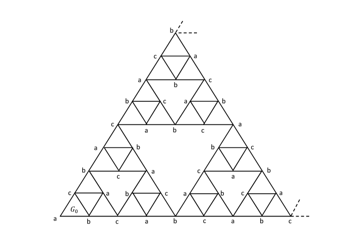
Figure 1. Labels on $\mathcal{V}_{0}.$

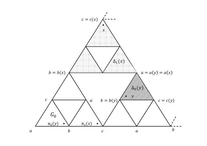
Figure 2. Illustration of the action of $\pi_{0}$ and $\pi_{1}$.

Let $M\geq 0$ be fixed. For $x\in\mathcal{G}\setminus\mathcal{V}_{M},$ there is a unique triangle of size $2^{M}$ that contains $x,$ $\Delta_{M}(x),$ and so $x$ can be written as $x=x_{a}a(x)+x_{b}b(x)+x_{c}c(x),$ where $a(x),$ $b(x),$ $c(x)$ are the vertices of $\Delta_{M}(x)$ with labels $a,b,c$ and $x_{a},x_{b},x_{c}\in(0,1),$ $x_{a}+x_{b}+x_{c}=1.$ Then we define the projection:

$$\mathcal{G}\setminus\mathcal{V}_{M}\ni x\mapsto\pi_{M}(x)=x_{a}\cdot a(M)+x_{b}\cdot b(M)+x_{c}\cdot c(M)\in\mathcal{G}_{M},$$

where $a(M),$ $b(M),$ $c(M)$ are the vertices of the triangle $\mathcal{G}_{M}$ with corresponding labels $a,b,c$ (see Fig. 2). When $x\in\mathcal{V}_{M},$ then $x$ itself has a label assigned and it then mapped onto the corresponding vertex of $\mathcal{G}_{M}.$

For every $M=0,1,2,...,$ the gasket $\mathcal{G}_{M+1}$ consists of $3$ isometric copies of $\mathcal{G}_{M}.$ These copies are denoted by $\mathcal{G}_{M}^{(i)},$ $i=1,2,3.$ For $i\neq j$ one has $m\left(\mathcal{G}_{M}^{(i)}\cap\mathcal{G}_{M}^{(j)}\right)=0$. Also, denote by $\pi_{M,i}$ the restriction of $\pi_{M}$ to $\mathcal{G}^{(i)}_{M}$.

2.2. The Brownian motion and subordinate processes on gaskets

2.2.1. Brownian motion

The Brownian motion on the two-sided infinite gasket (by the two-sided gasket we mean the set $\mathcal{G}^{*}=\mathcal{G}\cup i(\mathcal{G}),$ where $i$ is the reflection of $\mathbb{R}^{2}$ with respect to the $y-$axis) was first defined in [4]. It is a strong Markov and Feller process $\tilde{Z}=(\tilde{Z}_{t},\mathbf{P}_{x})_{t\geq 0,x\in\mathcal{G}^{*}}$, whose transition density with respect to the Hausdorff measure is symmetric in its space variables, continuous, and fulfils the following subgaussian estimates:

(2.2) $$c_{1}t^{-d_{s}/2}{\rm e}^{-c_{2}\left(\frac{d(x,y)}{t^{1/d_{w}}}\right)^{d_{w}/(d_{w}-1)}}\leq\tilde{g}(t,x,y)\leq c_{3}t^{-d_{s}/2}{\rm e}^{-c_{4}\left(\frac{d(x,y)}{t^{1/d_{w}}}\right)^{d_{w}/(d_{w}-1)}}\hskip-28.45274pt,$$

$$\phantom{}\hskip 199.16928pt\quad x,y\in\mathcal{G}^{*},\quad t>0,$$

with positive constants $c_{1},...,c_{4}.$ It is not hard to see that the Brownian motion $Z$ on the one-sided Sierpiński gasket $\mathcal{G}$ obtained from $\tilde{Z}$ by the projection $\mathcal{G}^{*}\to\mathcal{G}$, whose transition density is equal to $g(t,x,y)=\tilde{g}(t,x,y)+\tilde{g}(t,x,i(y))$ for $x\neq 0$ and twice this quantity when $x=0,$ shares all these properties, the subgaussian estimates included (with possibly worse constants $c_{i}$). We stick to the estimate (2.2) for $g(t,x,y)$ as well.

2.2.2. Subordinate Brownian motion

Let $S=(S_{t},\mathbf{P})_{t\geq 0}$ be a subordinator, i.e. an increasing Lévy process taking values in $[0,\infty]$ with $S_{0}=0$. The law of $S$, which will be denoted by $\eta_{t}({\rm d}u)$, is determined by the Laplace transform $\int_{0}^{\infty}{\rm e}^{-\lambda s}\eta_{t}({\rm d}s)={\rm e}^{-t\phi(\lambda)},$ $\lambda>0.$ The function $\phi:(0,\infty)\to[0,\infty)$ is called the Laplace exponent of $S$ and it has the representation

(2.3) $$\phi(\lambda)=b\lambda+\int_{0}^{\infty}(1-{\rm e}^{-\lambda s})\nu({\rm d}s),$$

where $b\geq 0$ is called the drift term and $\nu$, called the Lévy measure of $S$, is a $\sigma$-finite measure on $(0,\infty)$ satisfying $\int_{0}^{\infty}(s\wedge 1)\nu({\rm d}s)<\infty$. It is well known that when a function $\phi:(0,\infty)\to\mathbb{R}$ satisfies $\lim_{\lambda\to 0^{+}}\phi(\lambda)=0$ then it has can be represented by (2.3) if and only if it is a Bernstein function [34]. If the measure $\eta_{t}({\rm d}u)$ is absolutely continuous with respect to the Lebesgue measure, then the corresponding density is denoted by $\eta_{t}(u)$. For more properties of subordinators and Bernstein functions we refer to [5, 6, 34].

We always assume that $Z$ and $S$ are independent. The process $X=(X_{t},\mathbf{P}_{x})_{t\geq 0,x\in\mathcal{G}}$ given by

$$X_{t}:=Z_{S_{t}},\quad t\geq 0,$$

is called the subordinate Brownian motion on $\mathcal{G}$ (via subordinator $S$). It is also a symmetric Markov process with respect to its natural filtration (assumed to fulfil the usual conditions), with càdlàg paths. Its transition probabilities are given by

$$p(t,x,A)=\int_{0}^{\infty}\int_{A}g(u,x,y)m({\rm d}y)\eta_{t}({\rm d}u),\quad t>0,\quad x\in\mathcal{G},\quad A\in\mathcal{B}(\mathcal{G}).$$

Throughout the paper we impose some assumptions on the subordinator $S$ which provide sufficient regularity of the process $X$.

Assumption 2.1.

For every $t>0$ the following holds.

• (2.4) $$\eta_{t}(\left\{0\right\})=0\quad\text{and}\quad\int_{0^{+}}^{\infty}\frac{1}{u^{d_{s}/2}}\,\mathbb{\eta}_{t}({\rm d}u)=:c_{0}(t)<\infty.$$

• (2.5) $${\int_{1}^{\infty}\eta_{t}(u,\infty)\frac{{\rm d}u}{u}<\infty.}$$

It is clear that when $S_{t}=t$ and $X_{t}=Z_{t}$ (in this case, $\eta_{t}({\rm d}u)=\delta_{t}({\rm d}u)$ and $\phi(\lambda)=\lambda$), then both conditions (2.4) and (2.5) are satisfied.

Remark 2.1.

• The condition (2.5) is tantamount to $\sum_{M=1}^{\infty}\eta_{t}(a^{M},\infty)<\infty$, for every $a>1$. This summation property will be often explicitly used below. Moreover, one can verify that (2.5) holds when $\int_{1}^{\infty}\log u\ \eta_{t}({\rm d}u)<\infty$ for all $t>0$.

• In most cases, the measure $\eta_{t}(\cdot)$ is not explicitly given, but the corresponding Laplace exponent $\phi$ is known. In this case, very often, the integral condition in (2.4) can be verified by using Tauberian theorems of exponential type (see, e.g., [17, 21]). For example, when $\phi(\lambda)\geq c\lambda^{\gamma}$ for all $\lambda>\lambda_{0}$ with some $c,\lambda_{0}>0$ and $\gamma\in(0,1)$, then by [17, Theorem 2.1 (ii)] for every $t>0$ there is $\tilde{c}>0$ such that $\eta_{t}(0,u]\leq e^{-\tilde{c}u^{-\gamma/(1-\gamma)}}$ for sufficiently small $u>0$, and the integral condition in (2.4) holds. Furthermore, when $\phi$ is unbounded (in this case $S$ is not a compound Poisson process, see [5]), then for every $t>0$ the distribution of $S$ does not charge $\left\{0\right\}$, which is exactly the first part of (2.4). Also, in Lemma 2.2 below, we give a simple estimate which may be used in verification of (2.5) when $\phi$ is known.

Lemma 2.2.

Let $S$ be a subordinator with Laplace exponent $\phi$ and law $\eta_{t}(du)$ such that $\eta_{t}(\left\{0\right\})=0$ for every $t>0$. Then we have

$$\int_{1}^{\infty}\eta_{t}(u,\infty)\frac{{\rm d}u}{u}\leq t\int_{0}^{1}\frac{\phi(\lambda)}{\lambda}\,{\rm d}\lambda+e^{-1},\quad t>0.$$

Proof.

Fix $t>0$. Direct integration by parts gives for every $\lambda>0$ that

$$e^{-t\phi(\lambda)}=\int_{0}^{\infty}e^{-\lambda u}\eta_{t}({\rm d}u)=\lambda\int_{0}^{\infty}e^{-\lambda u}\eta_{t}(0,u]\,{\rm d}u\leq 1-\lambda\int_{1}^{\infty}e^{-\lambda u}\eta_{t}(u,\infty)\rm{d}u,$$

and, consequently,

$$\int_{1}^{\infty}e^{-\lambda u}\eta_{t}(u,\infty){\rm d}u\leq\frac{1-e^{-t\phi(\lambda)}}{\lambda}\leq\frac{t\phi(\lambda)}{\lambda}.$$

By integrating this inequality in $\lambda$ over the interval $(0,1)$ and changing the order of integrals on the left hand side, we finally get

$$\int_{1}^{\infty}\eta_{t}(u,\infty)\frac{{\rm d}u}{u}\leq t\int_{0}^{1}\frac{\phi(\lambda)}{\lambda}\,{\rm d}\lambda+e^{-1},$$

which completes the proof. ∎

Our Assumption 2.1 is satisfied by a wide class of subordinators. Below we discuss only several examples which are of special interest. For further examples we refer the reader to [7, 34].

Example 2.1.

In some cases, the densities of measures $\eta_{t}$ exist and precise bounds for them are known. However, for all examples listed here the Laplace exponent $\phi$ is explicitly given and Assumption 2.1 can be verified by using Lemma 2.2 and Tauberian theorems.

• $\alpha/d_{w}$-stable subordinators. Let $\phi(\lambda)=\lambda^{\alpha/d_{w}}$, $\alpha\in(0,d_{w}]$. It is well known that in this case the measure $\eta_{t}({\rm d}u)$ is absolutely continuous with respect to Lebesgue measure, the scaling property $\eta_{t}(u)=t^{-d_{w}/\alpha}\eta_{1}(t^{-d_{w}/\alpha}u)$ holds, and $\eta_{1}(u)\approx c(\alpha)u^{-1-\alpha/d_{w}}$, when $u\to\infty$. When $\alpha\in(0,d_{w})$, then the subordination via such subordinator leads to the purely jump process $X$ which is called $\alpha$-stable process on $\mathcal{G}$. The case $\alpha=d_{w}$ is different. As mentioned just after Assumption 2.1, in this case the process $Z$ remains unchanged. For properties of the subordinate $\alpha$-stable processes we refer to [9, 19] (cf. also [14]).

• Mixture of several purely jump stable subordinators. Let $\phi(\lambda)=\sum_{i=1}^{n}\lambda^{\alpha_{i}/d_{w}}$, $\alpha_{i}\in(0,d_{w})$, $n\in\mathbb{N}$. Many of basic properties of the process subordinated via this subordinator can be established in a similar way as in [9].

• $\alpha/d_{w}$-stable subordinator with drift. Let $\phi(\lambda)=b\lambda+\lambda^{\alpha/d_{w}}$, $\alpha\in(0,d_{w})$, $b>0$. Then the corresponding subordinator is a sum of a pure drift subordinator $bt$ and the purely jump $\alpha/d_{w}$-stable subordinator. In this case, $\phi(\lambda)\approx\lambda$ for $\lambda\to 0^{+}$, and $\phi(\lambda)\approx\lambda^{\alpha/d_{w}}$ for $\lambda\to\infty$.

• Relativistic $\alpha/d_{w}$-stable subordinator. Let $\phi(\lambda)=(\lambda+\mu^{d_{w}/\alpha})^{\alpha/d_{w}}-\mu$, $\alpha\in(0,d_{w})$, $\mu>0$. The subordination via such a subordinator leads to the so-called relativistic $\alpha$-stable process on $\mathcal{G}$. Since $\phi(\lambda)\approx\lambda$ for $\lambda\to 0^{+}$, and $\phi(\lambda)\approx\lambda^{\alpha/d_{w}}$ for $\lambda\to\infty$, similarly as before, Assumption 2.1 is satisfied.

• If $S$ is a subordinator with Laplace exponent $\phi(\lambda)=\lambda^{\alpha/d_{w}}[\log(1+\lambda)]^{\beta/d_{w}}$, $\alpha\in(0,d_{w})$, $\beta\in(-\alpha,0)$ or $\beta\in(0,d_{w}-\alpha)$, then Assumption 2.1 also holds.

An important consequence of the first part of assumption (2.4) is that the process $X$ has symmetric and strictly positive transition densities given by

(2.6) $$p(t,x,y)=\int_{0}^{\infty}g(u,x,y)\eta_{t}({\rm d}u),\quad t>0,\quad x,y\in\mathcal{G}.$$

The second part of this condition guarantees that

(2.7) $$\sup_{x,y\in\mathcal{G}}p(t,x,y)\leq c_{3}c_{0}(t)<\infty,$$

that for each fixed $t>0$, $p(t,\cdot,\cdot)$ is a continuous function on $\mathcal{G}\times\mathcal{G}$, and for each fixed $x,y\in\mathcal{G}$, $p(\cdot,x,y)$ is a continuous function on $(0,\infty)$.

By general theory of subordination (see, e.g., [34, Chapter 12]) the process $X$ is a Feller process and, in consequence, a strong Markov process. It is also easy to check that by (2.4) it has the strong Feller property.

Under the assumption (2.5) we obtain the following regularity for suprema of the subordinate process. It will be pivotal for our further investigations.

Lemma 2.3.

Let the condition (2.5) of Assumption 2.1 hold. Then for every $t>0$ and $a>1$ we have

(2.8) $$\sum_{M=1}^{\infty}\sup_{x\in\mathcal{G}}\mathbf{P}_{x}[\sup_{s\leq t}d(X_{s},x)>a^{M}]<\infty.$$

Proof.

Observe that for every $x\in\mathcal{G}$, $r>0$ and $t>0$ we have, since $S_{0}(w)=0$ a.s.,

$$\left\{w:\sup_{s\leq t}d(Z_{S_{s}(w)}(w),Z_{S_{0}(w)}(w))>r\right\}\subseteq\left\{w:\sup_{s\leq S_{t}(w)}d(Z_{s}(w),Z_{0}(w))>r\right\}.$$

This and [1, formula (3.21)] thus yield that for every $x\in\mathcal{G}$

$$\mathbf{P}_{x}[\sup_{s\leq t}d(X_{s},x)>r] \leq\mathbf{P}_{x}[\sup_{s\leq S_{t}}d(Z_{s},x)>r]\leq c_{1}\int_{0}^{\infty}{\rm e}^{-c_{2}\left(ru^{-1/d_{w}}\right)^{d_{w}/(d_{w}-1)}}\eta_{t}({\rm d}u)$$

$$=c_{1}\int_{0}^{r^{d_{w}/2}}+c_{1}\int_{r^{d_{w}/2}}^{\infty}\leq c_{1}{\rm e}^{-c_{2}r^{d_{w}/(2(d_{w}-1))}}+c_{1}\eta_{t}(r^{d_{w}/2},\infty).$$

By (2.5), the latter sum for $r=a^{M}$ is a term of a convergent series. ∎

For an open bounded set $D\subset\mathcal{G}$ by $\tau_{D}:=\inf\left\{t\geq 0:X_{t}\notin D\right\}$ we denote the first exit time of the process $X$ from $D$. We will need the following fact on the mean exit time for balls.

Lemma 2.4.

We have $\lim_{r\to 0^{+}}\sup_{x\in\mathcal{G}}\mathbf{E}_{x}\tau_{B(x,r)}=0$.

Proof.

As in [1, Lemma 3.9(c)] or [9, Prop. 2.14] we write, for any $t>0,$ $x\in\mathcal{G}$

$$\mathbf{P}_{x}[{\tau_{B(x,r)}}>t] \leq \mathbf{P}_{x}[X_{t}\in B(x,r)]=\int_{B(x,r)}p(t,x,y)\,{\rm d}y$$

$$\leq m(B(x,r))\sup_{y\in\mathcal{G}}p(t,x,y)\leq c_{3}r^{d_{f}}c_{0}(t)=:a(r,t_{0}).$$

From Markov property we get, for $k=1,2,...$

$$\mathbf{P}_{x}[\tau_{B(x,r)}>kt_{0}]\leq a(r,t_{0})^{k},$$

and, as long as $a(r,t_{0})<1,$

$$\mathbf{E}_{x}[\tau_{B(x,r)}] = \int_{0}^{\infty}\mathbf{P}_{x}[\tau_{B(x,r)}>t]{\rm d}t=\int_{0}^{t_{0}}\mathbf{P}_{x}[\tau_{B(x,r)}>t]{\rm d}t+t_{0}\sum_{k=1}^{\infty}\mathbf{P}_{x}[\tau_{B(x,r)}>kt_{0}]$$

$$\leq \frac{t_{0}}{1-a(r,t_{0})}.$$

Fix $\epsilon>0$ and $t_{0}={\epsilon}.$ For $r<r_{0}(\epsilon)=(2c_{3}c_{0}(\epsilon))^{-1/d_{f}})$ we get $\frac{1}{1-a(r,t_{0})}<2,$ and thus for any $x\in\mathcal{G}$ $\mathbf{E}_{x}[\tau_{B(x,r)}]\leq 2\epsilon,$ which completes the proof. ∎

By $\mathbf{P}^{t}_{x,y}$ we denote the bridge measure with respect to process $X$ on $D([0,t],\mathcal{G})$, i.e. the measure concentrated on càdlàg paths of $X$ which start from $x\in\mathcal{G}$ at time $0$ and end at $y\in\mathcal{G}$ at time $t>0$. Subordinate process $X$ is a Feller process with sufficiently regular transition densities, and therefore in our case such a measure always exists (see [13] and references therein). Formally, for every $x,y\in\mathcal{G}$ and $t>0$ the measure $\mathbf{P}^{t}_{x,y}$ is the conditional law of the process $(X_{s})_{0\leq s\leq t}$ given $X_{t}=y$ under $\mathbf{P}_{x},$ such that for every $0\leq s<t$ and $A\in\sigma(X_{s}:0\leq u\leq s)$ we have

(2.9) $$p(t,x,y)\mathbf{P}^{t}_{x,y}(A)=\mathbf{E}_{x}\left[\mathbf{1}_{A}p(t-s,X_{s},y)\right].$$

Moreover, an essential consequence of the Feller property of $X$ is that after performing the integration with respect to $m({\rm d}y)$, (2.9) extends to $s=t$. Indeed, for every bounded Borel function $f$ and $A\in\sigma(X_{s}:0\leq u\leq t)$ we have

(2.10) $$\mathbf{E}_{x}\left[\mathbf{1}_{A}f(X_{t})\right]=\int_{\mathcal{G}}\mathbf{E}^{t}_{x,y}\left[\mathbf{1}_{A}\right]f(y)p(t,x,y)m({\rm d}y),\quad x\in\mathcal{G}.$$

For justification of (2.10) we refer to [13, Section 3]. Since $p(t,x,y)=p(t,y,x)$ for $x,y\in\mathcal{G}$ and $t>0$, the processes $\left((X_{s})_{0\leq s\leq t},\mathbf{P}^{t}_{x,y}\right)$ and $\left((X_{t-s})_{0\leq s\leq t},\mathbf{P}^{t}_{y,x}\right)$ are indentical in law. Below we will refer to this property as the symmetry of the brigde measure.

2.2.3. The reflected process

The processes we will be mostly working with are the reflected subordinate Brownian motions on $\mathcal{G}_{M},$ defined by

$$X_{t}^{M}=\pi_{M}(X_{t}),$$

where $\pi_{M}$ is the projection $\mathcal{G}\to\mathcal{G}_{M},$ described in Section 2.1. Similar process based on the ordinary Brownian motion on $\mathcal{G}^{*}$ was studied in [30]. Only $M=0$ was considered there, but for arbitrary $M$ the properties of the reflected Brownian motion are similar. Also, the construction of the reflected Brownian motion from the Brownian motion on $\mathcal{G}$ instead of $\mathcal{G}^{*}$ leads to the same process. The process $Z_{t}^{M}=\pi_{M}(Z_{t})$ has strictly positive and symmetric transition densities with respect to $m,$ which are given by the formula

$$g^{M}(t,x,y)=\left\{\begin{array}[]{ll}\sum_{y^{\prime}\in\pi_{M}^{-1}(y)}g(t,x,y^{\prime}),&\mbox{when }x,y\in\mathcal{G}_{M},\,y\notin\mathcal{V}_{M}\setminus\{0\},\\[5.69054pt] 2\sum_{y^{\prime}\in\pi_{M}^{-1}(y)}g(t,x,y^{\prime}),&\mbox{when }x\in\mathcal{G}_{M},\,y\in\mathcal{V}_{M}\backslash\left\{0\right\}.\end{array}\right.$$

For each fixed $M\in\mathbb{Z}_{+}$ the function $g^{M}(t,x,y)$ is jointly continuous in $(t,x,y)$ and symmetric in its space variables. This was proved in [30, Lemma 4 and Lemma 7] for $M=0$, but the same arguments directly extend to any $M\in\mathbb{Z}_{+}$. Similarly, we put

$$p^{M}(t,x,y)=\left\{\begin{array}[]{ll}\sum_{y^{\prime}\in\pi_{M}^{-1}(y)}p(t,x,y^{\prime}),&\mbox{when }x,y\in\mathcal{G}_{M},\,y\notin\mathcal{V}_{M}\setminus\{0\},\\[5.69054pt] 2\sum_{y^{\prime}\in\pi_{M}^{-1}(y)}p(t,x,y^{\prime}),&\mbox{when }x\in\mathcal{G}_{M},\,y\in\mathcal{V}_{M}\backslash\left\{0\right\}.\end{array}\right.$$

It is an easy observation that the projection commutes with subordination, i.e. the formula

(2.11) $$p^{M}(t,x,y)=\int_{0}^{\infty}g^{M}(u,x,y)\eta_{t}({\rm d}u),\;\;\;x,y\in\mathcal{G}_{M},\;t>0,$$

defines the transition densities of the symmetric Markov process $X^{M}$. To discuss further properties of the reflected process $X^{M}$ we need the following lemma.

Lemma 2.5.

For each fixed $t>0$ one has:

• (2.12) $$\sup_{x,y\in\mathcal{G}_{M}}\sum_{\stackrel{{\scriptstyle y^{{}^{\prime}}\in\pi^{-1}_{M}(y)}}{{y^{\prime}\notin\mathcal{G}_{M+1}}}}g(t,x,y^{\prime})\leq C{2^{-Md_{f}}}\left(\frac{2^{M}}{t^{1/d_{w}}}\vee 1\right)^{d_{f}-\frac{d_{w}}{d_{w}-1}}{\rm e}^{-\tilde{c}_{4}\left(\frac{2^{M}}{t^{1/d_{w}}}\vee 1\right)^{\frac{d_{w}}{d_{w}-1}}},\quad M\in\mathbb{Z_{+}},$$

  with certain numerical constant $C>0$ and $\tilde{c}_{4}=\frac{c_{4}}{2^{d_{w}/(d_{w}-1)}}.$ In particular, there is a universal constant $c_{5}>0$ such that

  (2.13) $$g^{M}(t,x,y)\leq c_{5}{(t^{-d_{s}/2}\vee 2^{-Md_{f}})},\quad x,y\in\mathcal{G}_{M},\quad t>0,\quad M\in\mathbb{Z_{+}}.$$

• For

  (2.14) $$C(M,t):=\sup_{x,y\in\mathcal{G}_{M}}\sum_{\stackrel{{\scriptstyle y^{{}^{\prime}}\in\pi^{-1}_{M}(y)}}{{y^{\prime}\notin\mathcal{G}_{M+1}}}}p(t,x,y^{\prime}),\quad t>0,\quad M\in\mathbb{Z_{+}},$$

  one has

  $$\sum_{M=1}^{\infty}C(M,t)<\infty.$$

  In particular, $C(M,t)\to 0$ as $M\to\infty$.

Proof.

Let $x,y\in\mathcal{G}_{M}$. All the points $y^{\prime}$ from the sums below are taken from the fiber of $y.$

(a) One can write

$$\sum_{y^{\prime}\notin\mathcal{G}_{M+1}}g(t,x,y^{\prime})=\sum_{k\geq 1}\;\sum_{y^{\prime}\in\mathcal{G}_{M+k+1}\setminus\mathcal{G}_{M+k}}p(t,x,y^{\prime}).$$

When $y^{\prime}\in\mathcal{G}_{M+k+1}\setminus\mathcal{G}_{M+k},$ then $d(y^{\prime},0)\geq 2^{M+k},$ and since $d(x,0)\leq 2^{M},$ we have $d(y^{\prime},x)\geq\frac{1}{2}2^{M+k}.$ The number of such points $y^{\prime}$ is not bigger than the number of $M-$triangles in $\mathcal{G}_{M+k+1}\setminus\mathcal{G}_{M+k},$ i.e. $2\cdot{3^{k}}.$ Therefore from the subgaussian estimate on $g$ we get:

$$\sum_{y^{\prime}\notin\mathcal{G}_{M+1}}g(t,x,y^{\prime})\leq\frac{2c_{3}}{{2^{Md_{f}}}t^{d_{s}/2}}\sum_{k\geq 1}3^{M+k}{\rm e}^{-c_{4}\left(\frac{2^{M+k}}{2t^{1/d_{w}}}\right)^{\frac{d_{w}}{d_{w}-1}}}=(*).$$

Since for any $C,\gamma>0$ the function $x\mapsto{\rm e}^{-Cx^{\gamma}}$ is monotone decreasing, we can estimate the series above by an appropriate integral, getting that

$$(*)\leq\frac{\tilde{c}_{3}}{{2^{Md_{f}}}t^{d_{s}/2}}\int_{3^{M}}^{\infty}{\rm e}^{-\tilde{c}_{4}\left(\frac{x^{1/d_{f}}}{t^{1/d_{w}}}\right)^{\frac{d_{w}}{d_{w}-1}}}\,{\rm d}x=\frac{\tilde{c}_{3}d_{f}}{{2^{Md_{f}}}}\int_{2^{M}t^{-\frac{1}{d_{w}}}}^{\infty}y^{d_{f}-1}{\rm e}^{-\tilde{c}_{4}y^{\frac{d_{w}}{d_{w}-1}}}{\rm d}y,$$

where we have denoted $\tilde{c}_{4}=\frac{c_{4}}{2^{\frac{d_{w}}{d_{w}-1}}}.$ Using an elementary estimate

$$\int_{a}^{\infty}y^{\beta}{\rm e}^{-\eta y^{\gamma}}{\rm d}y\leq C(a\vee 1)^{\beta-\gamma+1}{\rm e}^{-\eta(a\vee 1)^{\gamma}},\quad\eta,\beta,\gamma>0,$$

we can write

$$\sum_{y^{\prime}\notin\mathcal{G}_{M+1}}g(t,x,y^{\prime})\leq C{2^{-Md_{f}}}\left(\frac{2^{M}}{t^{1/d_{w}}}\vee 1\right)^{d_{f}-\frac{d_{w}}{d_{w}-1}}{\rm e}^{-\tilde{c}_{4}\left(\frac{2^{M}}{t^{1/d_{w}}}\vee 1\right)^{\frac{d_{w}}{d_{w}-1}}},$$

with certain numerical constant $C>0,$ getting (2.12).

To see (2.13), first observe that, given $y\in\mathcal{G}_{M},$ there are at most 3 points in $\pi^{-1}_{M}(y)\cap\mathcal{G}_{M+1},$ so that, using (2.2) and (2.12) we get

$$\sup_{x,y\in\mathcal{G}_{M}}g^{M}(t,x,y)\leq\frac{4c_{3}}{t^{d_{s}/2}}+C{2^{-Md_{f}}}\left(\frac{2^{M}}{t^{1/d_{w}}}\vee 1\right)^{d_{f}-\frac{d_{w}}{d_{w}-1}}{\rm e}^{-\tilde{c}_{4}\left(\frac{2^{M}}{t^{1/d_{w}}}\vee 1\right)^{\frac{d_{w}}{d_{w}-1}}}.$$

When $t\geq 5^{M},$ then this is bounded by $\frac{4c_{3}}{2^{Md_{f}}}+\frac{C{\rm e}^{-\tilde{c}_{4}}}{2^{Md_{f}}}=:\frac{c}{2^{Md_{f}}}$. On the other hand, for $t\leq 5^{M},$ denoting $a=\frac{2^{M}}{t^{1/d_{w}}}\geq 1$ we observe

$$a^{d_{f}-\frac{d_{w}}{d_{w}-1}}{\rm e}^{-\tilde{c}_{t}a^{\frac{d_{w}}{d_{w}-1}}}\leq a^{d_{f}}{\rm e}^{-\tilde{c}_{4}}={\rm e}^{-\tilde{c}_{4}}\,\frac{{2^{Md_{f}}}}{t^{d_{f}/d_{w}}}.$$

Once we note that $d_{f}/d_{w}=d_{s}/2,$ this is exactly what is needed to get (2.13).

(b) We now integrate the bound (2.12) against the distribution of $S_{t},$ getting

$$\sum_{y^{\prime}\notin\mathcal{G}_{M+1}}p(t,x,y^{\prime}) \leq C\int_{0}^{5^{M}}\left(\frac{2^{M}}{u^{1/d_{w}}}\right)^{d_{f}-\frac{d_{w}}{d_{w}-1}}{\rm e}^{-\tilde{c}_{4}\left(\frac{2^{M}}{u^{1/d_{w}}}\right)^{\frac{d_{w}}{d_{w}-1}}}\eta_{t}({\rm d}u)$$

$$+C\int_{5^{M}}^{\infty}{\rm e}^{-\tilde{c}_{4}}\eta_{t}({\rm d}u)$$

$$=: A(M,t)+C\ {\eta_{t}(5^{M},\infty)}=:C(M,t).$$

In view of (2.5) (see Remark 2.1 (1)), to get $\sum_{M}C(M,t)<\infty,$ it is enough to check that $\sum_{M}A(M,t)<\infty.$ To shorten the notation, write $\gamma=d_{f}-\frac{d_{w}}{d_{w}-1}.$ We have

$$\sum_{M=1}^{\infty}A_{M}(t) \leq \sum_{M=1}^{\infty}\int_{0}^{5^{M}}\left(\frac{2^{M}}{u^{1/d_{w}}}\right)^{\gamma}{\rm e}^{-\tilde{c}_{4}\left(\frac{2^{M}}{u^{1/d_{w}}}\right)^{\frac{d_{w}}{d_{w}-1}}}\eta_{t}({\rm d}u)$$

$$= \sum_{M=1}^{\infty}\sum_{n=1}^{\infty}\int_{5^{M-n-1}}^{5^{M-n}}\left(\frac{2^{M}}{u^{1/d_{w}}}\right)^{\gamma}{\rm e}^{-\tilde{c}_{4}\left(\frac{2^{M}}{u^{1/d_{w}}}\right)^{\frac{d_{w}}{d_{w}-1}}}\eta_{t}({\rm d}u)$$

$$\leq C\sum_{M}\sum_{n}2^{n\gamma}{\rm e}^{-\tilde{c}_{4}2^{\frac{nd_{w}}{d_{w}-1}}}{\eta_{t}(5^{M-n-1},5^{M-n}]}$$

$$= \sum_{n}2^{n\gamma}{\rm e}^{-\tilde{c}_{4}2^{\frac{nd_{w}}{d_{w}-1}}}{\eta_{t}(5^{-n},\infty)}<\infty,$$

which completes the proof.

∎

Thanks to the second part of the assumption (2.4), (2.11) and (2.13), the kernel $p^{M}(t,x,y)$ has the same continuity properties as $p(t,x,y)$. Also,

$$\sup_{x,y\in\mathcal{G}}p^{M}(t,x,y)\leq c(M,t)<\infty.$$

Furthermore, it is easy to see that for each fixed $M\in\mathbb{Z}_{+}$ the process $X^{M}$ is Feller and strong Feller, and, therefore, again, we may and do consider the corresponding bridge process (see [13]). Similarly as before, by $\mathbf{P}^{M,t}_{x,y}$, $M\in\mathbb{Z}_{+}$, $t>0$, $x,y\in\mathcal{G}_{M}$, we denote the bridge measure of the process $(X^{M}_{s})_{0\leq s\leq t}$ on $D([0,t],\mathcal{G}_{M})$, satisfying the usual bridge property: for every $0\leq s<t$ and $A\in\sigma(X^{M}_{s}:0\leq u\leq s)$ we have

(2.16) $$p^{M}(t,x,y)\mathbf{P}^{M,t}_{x,y}(A)=\mathbf{E}_{x}\left[\mathbf{1}_{A}p^{M}(t-s,X_{s},y)\right].$$

Similarly as for the process $X$ (see (2.10)), thanks to the Feller property of $X^{M}$, (2.16) extends to $s=t$ after performing the integration with respect to $m({\rm d}y)$. Moreover, the bridge measures for the reflected and the ordinary subordinate process are related through the following identity.

Lemma 2.6.

(a) For every $t>0$, $x,y\in\mathcal{G}\setminus\mathcal{V}_{M}$, $M\in\mathbb{Z_{+}}$ and the set $A\in\mathcal{B}(D[0,t],\mathcal{G}_{M})$ we have

(2.17) $$p^{M}(t,\pi_{M}(x),\pi_{M}(y))\mathbf{P}^{M,t}_{\pi_{M}(x),\pi_{M}(y)}[A]=\sum_{y^{\prime}\in\pi_{M}^{-1}(\pi_{M}(y))}p(t,x,y^{\prime})\mathbf{P}^{t}_{x,y^{\prime}}[\pi_{M}^{-1}(A)]$$

(b) Consequently, for any $i=1,2,3$ and $x\in\mathcal{G}_{M},$

$$\sum_{x^{{}^{\prime}}\in\pi^{-1}_{M}(x)}p(t,\pi^{-1}_{M,i}(x),x^{\prime})\mathbf{E}^{t}_{\pi^{-1}_{M,i}(x),x^{{}^{\prime}}}\left[\pi^{-1}_{M}(A)\right]=\sum_{x^{{}^{\prime}}\in\pi^{-1}_{M}(x)}p(t,x,x^{\prime})\mathbf{E}^{t}_{x,x^{{}^{\prime}}}\left[\pi^{-1}_{M}(A)\right].$$

Proof.

(a) This is a consequence of Theorem 3 in [30]. For the Brownian density one has

(2.18) $$\sum_{z^{\prime}\in\pi_{M}^{-1}(z)}g(t,x,z^{\prime})=\sum_{z^{\prime}\in\pi_{M}^{-1}(z)}g(t,y,z^{\prime}),$$

whenever $z\in\mathcal{G}_{M}$ and $x,y\in\mathcal{G}$ are such points that $\pi_{M}(x)=\pi_{M}(y)$ (the proof in [30] is carried for $M=0$ only; the general case is similar). Integrating this against $\eta_{t}$ we get identical property for $p(\cdot,\cdot,\cdot).$ Now, as it was done in [30, Lemma 8], it is enough to check the relation (2.17) for cylindrical sets only. This is straightforward using property (2.18) for $p.$ To get (b) just observe that $\pi_{M}(\pi_{M,i}^{-1}(x))=x$ and then use (2.17). ∎

In the sequel, we will need the following trace type property.

Lemma 2.7.

For every $t>0$,

(2.19) $$\sum_{M=1}^{\infty}\frac{1}{m(\mathcal{G}_{M})}\int_{\mathcal{G}_{M}}\left|p(t,x,x)-p^{M}(t,x,x)\right|m({\rm d}x)<\infty.$$

In particular,

(2.20) $$\frac{1}{m(\mathcal{G}_{M})}\int_{\mathcal{G}_{M}}\left|p(t,x,x)-p^{M}(t,x,x)\right|m({\rm d}x)\to 0,\quad\text{as}\quad M\to\infty.$$

Proof.

We can write, with all the points $x^{\prime}$ taken from the fiber of $x,$

$$\frac{1}{m(\mathcal{G}_{M})}\int_{\mathcal{G}_{M}}|p^{M}(t,x,x)-p(t,x,x)|\,m({\rm d}x) \leq \frac{2}{m(\mathcal{G}_{M})}\int_{\mathcal{G}_{M}}\sup_{x^{\prime}\in\mathcal{G}_{M+1}\setminus\mathcal{G}_{M}}p(t,x,x^{\prime})\,m({\rm d}x)$$

$$+\frac{1}{m(\mathcal{G}_{M})}\int_{\mathcal{G}_{M}}\sum_{x^{\prime}\notin\mathcal{G}_{M+1}}p(t,x,x^{\prime})\,m({\rm d}x)$$

$$=: \mathcal{A}_{M}+\mathcal{B}_{M}.$$

We have $\mathcal{B}_{M}\leq C(M,t)$ (recall $C(M,t)$ is defined in (2.14)), which is a term of a convergent series. Therefore it remains to prove that $\sum\mathcal{A}_{M}<\infty.$ We split the integral in $\mathcal{A}_{M}$ into two integrals: over $E_{M}^{1}=B(0,{2^{M}}\left(1-\frac{1}{M^{2}}\right))$ and over $E_{M}^{2}=\mathcal{G}_{M}\setminus E_{M}^{1}.$ Using (2.1), we can write

$$\frac{m(E_{M}^{2})}{m(\mathcal{G}_{M})}\leq\frac{c}{M^{2(d_{f}-1)}},$$

and since $p(t,x,x^{\prime})\leq c_{0}(t),$ and $2(d_{f}-1)>1,$ the part of the expression corresponding to the integral over $E^{2}_{M}$ is a term of a convergent series.

When $x\in E_{1}^{M},$ then for all $x^{\prime}\notin\mathcal{G}_{M}$ one has $d(x,x^{\prime})>\frac{2^{M}}{M^{2}}.$ From the subgaussian estimates and the subordination formula one gets

$$p(t,x,x^{\prime}) = \int_{0}^{\infty}g(u,x,x^{\prime})\eta_{t}({\rm d}u)\leq c_{3}\int_{0}^{\infty}\frac{1}{u^{d_{s}/2}}\,{\rm e}^{-c_{4}\left(\frac{2^{M}}{M^{2}\cdot u^{1/d_{w}}}\right)^{\frac{d_{w}}{d_{w}-1}}}\eta_{t}({\rm d}u)$$

It follows

$$\frac{1}{m(\mathcal{G}_{M})}\int_{E^{1}_{M}}\sup_{x^{\prime}\in\mathcal{G}_{M+1}\setminus\mathcal{G}_{M}}p(t,x,x^{\prime})\,m({\rm d}x)\leq c_{3}\int_{0}^{\infty}\frac{1}{u^{d_{s}/2}}\,{\rm e}^{-c_{4}\left(\frac{2^{M}}{M^{2}\cdot u^{1/d_{w}}}\right)^{\frac{d_{w}}{d_{w}-1}}}\eta_{t}({\rm d}u).$$

Summing these integrals up, we obtain that

$$\sum_{M\geq 1}\mathcal{A}_{M}\leq\sum_{M\geq 1}\frac{c}{M^{2}}+c_{3}\int_{0}^{\infty}\frac{1}{u^{d_{s}/2}}\sum_{M\geq 0}{\rm e}^{-c_{4}\left(\frac{2^{M+1}}{(M+1)^{2}u^{1/d_{w}}}\right)^{\frac{d_{w}}{d_{w}-1}}}\eta_{t}({\rm d}u).$$

We now take care of the sum under the integral sign. Again, we compare it with appropriate integrals. Observe that for $M\geq 3$

$$\int_{2^{M}/M^{2}}^{2^{(M+1)}/(M+1)^{2}}\frac{1}{x}\,{\rm e}^{-c_{4}\left(\frac{x}{u^{1/d_{w}}}\right)^{\frac{d_{w}}{d_{w}-1}}}{\rm d}x \geq \left(\frac{2^{M+1}}{(M+1)^{2}}-\frac{2^{M}}{M^{2}}\right)\frac{(M+1)^{2}}{2^{M+1}}\,{\rm e}^{-c_{4}\left(\frac{2^{M+1}}{(M+1)^{2}\cdot u^{1/d_{w}}}\right)^{\frac{d_{w}}{d_{w}-1}}}$$

$$\geq c\,{\rm e}^{-c_{4}\left(\frac{2^{M+1}}{(M+1)^{2}\cdot u^{1/d_{w}}}\right)^{\frac{d_{w}}{d_{w}-1}}}.$$

It follows that

$$\sum_{M\geq 0}\,{\rm e}^{-c_{4}\left(\frac{2^{M+1}}{(M+1)^{2}\cdot u^{1/d_{w}}}\right)^{\frac{d_{w}}{d_{w}-1}}} \leq 3+c\int_{8/9}^{\infty}{\rm e}^{-c_{4}\left(\frac{x}{u^{1/d_{w}}}\right)^{\frac{d_{w}}{d_{w}-1}}}\frac{{\rm d}x}{x},$$

and, consequently,

$$\sum_{M\geq 1}\mathcal{A}_{M}\leq c\left(1+\int_{0}^{\infty}\frac{\eta_{t}({\rm d}u)}{u^{d_{s}/2}}+\int_{0}^{\infty}\left[\int_{8/9}^{\infty}{\rm e}^{-c_{4}\left(\frac{x}{u^{1/d_{w}}}\right)^{\frac{d_{w}}{d_{w}-1}}}\frac{{\rm d}x}{x}\right]\frac{\eta_{t}({\rm d}u)}{u^{d_{s}/2}}\right).$$

According to Assumption 2.1 (see (2.4)), it suffices to show that the last double integral is convergent. By Fubini, we see that it is equal to

$$\int_{8/9}^{\infty}\left[\left(\int_{0}^{x}+\int_{x}^{\infty}\right){\rm e}^{-c_{4}\left(\frac{x}{u^{1/d_{w}}}\right)^{\frac{d_{w}}{d_{w}-1}}}\frac{\eta_{t}({\rm d}u)}{u^{d_{s}/2}}\right]\frac{{\rm d}x}{x}\leq\int_{8/9}^{\infty}{\rm e}^{-c_{4}x}\frac{{\rm d}x}{x}\ \cdot\ \int_{0}^{\infty}\frac{\eta_{t}({\rm d}u)}{u^{d_{s}/2}}+c\int_{8/9}^{\infty}\eta_{t}(x,\infty)\frac{{\rm d}x}{x}.$$

Again, by Assumption 2.1, the last two integrals above are convergent. We are done.

∎

2.3. Processes perturbed by Schrödinger potentials

2.3.1. Nonrandom Feynman-Kac semigroups

We say that a Borel function $V$ is in Kato class $\mathcal{K}^{X}$ related to the process $X$ if

(2.21) $$\lim_{t\searrow 0}\sup_{x\in\mathcal{G}}\int_{0}^{t}\mathbf{E}_{x}|V(X_{s})|\,{\rm d}s=0.$$

Also, $V\in\mathcal{K}^{X}_{\operatorname{loc}}$ (local Kato class), when $\mathbf{1}_{B}V\in\mathcal{K}^{X}$ for every ball $B\subset\mathcal{G}$. Obviously, $L^{\infty}_{\operatorname{loc}}(\mathcal{G})\subset\mathcal{K}^{X}_{\operatorname{loc}}$. Furthermore, it is a general fact that $\mathcal{K}_{\operatorname{loc}}^{X}\subset L^{1}_{\operatorname{loc}}(\mathcal{G},m)$. It is also useful to note that under the condition $\int_{0}^{1}c_{0}(t){\rm d}t<\infty$ (recall that the constant $c_{0}(t)$ was defined in $\eqref{eq:assum1}$), in fact one has $\mathcal{K}_{\operatorname{loc}}^{X}=L^{1}_{\operatorname{loc}}(\mathcal{G},m)$. Indeed, for $V\in L^{1}_{\operatorname{loc}}(\mathcal{G},m)$ and an arbitrary bounded Borel set $B\subset\mathcal{G}$ we get, using the subordination formula (2.6), estimate (2.2), and the assumption on $c_{0}$:

$$\sup_{x\in\mathcal{G}}\int_{0}^{t}\mathbf{E}_{x}|V(X_{s})\mathbf{1}_{B}(X_{s})|{\rm d}s\leq c\int_{0}^{t}\int_{0}^{\infty}u^{-d_{s}/2}\eta_{s}({\rm d}u){\rm d}s\cdot\int_{B}|V(y)|m({\rm d}y)\leq c_{1}\int_{0}^{t}c_{0}(s){\rm d}s\to 0$$

as $t\to 0^{+}$. Hence $V\in\mathcal{K}^{X}_{\operatorname{loc}}$.

Under our conditions on the process $X$, formula (2.21) can be rewritten as (see [41, Theorem 1])

(2.22) $$\lim_{\varepsilon\searrow 0}\sup_{x\in\mathcal{G}}\mathbf{E}_{x}\int_{0}^{\tau_{B(x,\varepsilon)}}|V(X_{s})|{\rm d}s=0.$$

The condition (2.22) is always very useful. For instance, when $V\in\mathcal{K}^{X}_{\operatorname{loc}}$ then by using (2.22) one can easily show that for every $M\in\mathbb{Z_{+}}$ we also have $V_{M}\in{\mathcal{K}^{X}}$, where $V_{M}$ is the usual periodization of $V$, i.e. $V_{M}(x):=V(\pi_{M}(x))$, $x\in\mathcal{G}$.

Under the condition $V\in\mathcal{K}^{X}_{\operatorname{loc}}$, we may define the Feynman-Kac semigroups related to the killed and the reflected process in $\mathcal{G}_{M}$, $M\in\mathbb{Z_{+}}$. Let

(2.23) $$T_{t}^{D,M}f(x)=\mathbf{E}_{x}\left[{\rm e}^{-\int_{0}^{t}V(X_{s}){\rm d}s}f(X_{t});t<\tau_{\mathcal{G}_{M}}\right],\quad f\in L^{2}(\mathcal{G}_{M},m),\quad M\in\mathbb{Z_{+}},\quad t>0,$$

and

(2.24) $$T_{t}^{N,M}f(x)=\mathbf{E}^{M}_{x}\left[{\rm e}^{-\int_{0}^{t}V(X^{M}_{s}){\rm d}s}f(X^{M}_{t})\right],\quad f\in L^{2}(\mathcal{G}_{M},m),\quad M\in\mathbb{Z_{+}},\quad t>0.$$

It is not very difficult to check that both semigroups $(T_{t}^{D,M})$ and $(T_{t}^{N,M})$ are ultracontractive. Since for every $t>0$, both operators $T_{t}^{D,M}$ and $T_{t}^{N,M}$ are also symmetric and bounded on $L^{2}(\mathcal{G}_{M})$, they admit measurable, symmetric and bounded kernels (see [35, Theorem A.1.1 and Corollary A.1.2]), i.e.

(2.25) $$T_{t}^{D,M}f(x)=\int_{\mathcal{G}_{M}}u^{M}_{D}(t,x,y)f(y)m({\rm d}y),\quad f\in L^{2}(\mathcal{G}_{M},m),\quad M\in\mathbb{Z_{+}},\quad t>0,$$

(2.26) $$T_{t}^{N,M}f(x)=\int_{\mathcal{G}_{M}}u^{M}_{N}(t,x,y)f(y)m({\rm d}y),\quad f\in L^{2}(\mathcal{G}_{M},m),\quad M\in\mathbb{Z_{+}},\quad t>0.$$

For verification of all basic properties of Feynman-Kac semigroups for Markov processes, including those listed above, we refer the reader to [16, Sections 3.2 and 3.3].

By (2.10) and its counterpart for the process $X^{M}$, one obtains the following very useful bridge representations for the kernels. We have

(2.27) $$u^{M}_{D}(t,x,y)=p(t,x,y)\ \mathbf{E}^{t}_{x,y}\left[{\rm e}^{-\int_{0}^{t}V(X_{s}){\rm d}s};t<\tau_{\mathcal{G}_{M}}\right],\quad M\in\mathbb{Z_{+}},\quad x,y\in\mathcal{G}_{M},\quad t>0,$$

(2.28) $$u^{M}_{N}(t,x,y)=p^{M}(t,x,y)\ \mathbf{E}^{M,t}_{x,y}\left[{\rm e}^{-\int_{0}^{t}V(X^{M}_{s}){\rm d}s}\right],\quad M\in\mathbb{Z_{+}},\quad x,y\in\mathcal{G}_{M},\quad t>0.$$

To shorten the notation, we will write $e_{V}(t):={\rm e}^{-\int_{0}^{t}V(\cdot){\rm d}s}$, $t>0$, for the Feynman-Kac functionals for both processes $X$ and $X^{M}$.

Generators of semigroups $(T_{t}^{D,M})$ and $(T^{N,M}_{t})$ will be denoted by $A^{M,D}$ and $A^{M,N}$, respectively. By analogy to the classical case, the operators $-A^{M,D}$ and $-A^{M,N}$ will be called the generalized Schrödinger operators corresponding to the generator of the process $X$. The first one, $-A^{M,D}$, is related to the killed process and therefore, in fact, it is a Schrödinger operator based on the generator of the process $X$ with Dirichlet (outer) conditions. Similarly, $-A^{M,N}$ may be seen as the Schrödinger operator based on the ‘Neumann’ generator of this process. Indeed, the process $X^{M}$ appears via the subordination of the reflected Brownian motion (recall (2.11)) and it can be regarded as a jump counterpart of the process ‘reflected on exiting the set $\mathcal{G}_{M}$’. Let us emphasize, however, that when the process has discontinuous trajectories, then there is no canonical definition of the ‘reflected process’ and there are several possible ways of constructing it.

As we pointed out above, for every $t>0$ and $M\in\mathbb{Z}_{+}$, both kernels $u^{M}_{D}(t,x,y)$ and $u^{M}_{N}(t,x,y)$ are bounded. Since also $m(\mathcal{G}_{M})<\infty$ for all $M\in\mathbb{Z}_{+}$, all operators $T_{t}^{D,M}$ and $T^{N,M}_{t}$ are of Hilbert-Schmidt type. Therefore, the spectra of the related Schrödinger operators, $-A^{M,D}$ and $-A^{M,N}$, consist only of eigenvalues of finite multiplicity having no accumulation points, and they can be ordered as $\lambda_{1}^{D,M}\leq\lambda_{2}^{D,M}\leq...$ and $\lambda_{1}^{N,M}\leq\lambda_{2}^{N,M}\leq...$. It is known that the corresponding eigenfunctions $(\phi^{D,M}_{n})_{n\geq 1}$ (resp. $(\phi^{N,M}_{n})_{n\geq 1}$) form a complete orthonormal system in $L^{2}(\mathcal{G},m)$.

2.3.2. Random potentials.

In the sequel, we will consider a more general case, when the potential $V$ is not a deterministic function. Let $(\Omega,\mathcal{M},\mathbb{Q})$ be a probability space and $V(x,\omega)$ – a real-valued function on $\mathcal{G}\times\Omega$ such that $V(x,\cdot)$ is measurable for each fixed $x\in\mathcal{G}$ and $V(\cdot,\omega)\in\mathcal{K}^{X}_{\operatorname{loc}}$ for $\mathbb{Q}$-almost all $\omega\in\Omega$. Such a function $V$ is called a random potential or a random field.

For a random potential $V(\cdot,\omega)$ which $\mathbb{Q}$-a.s. belongs to the local Kato class $\mathcal{K}^{X}_{\rm loc}$, we consider random Feynman-Kac semigroups $(T^{D,M,\omega}_{t})_{t\geq 0}$ and $(T^{N,M,\omega}_{t})_{t\geq 0},$ given by (2.23)-(2.24). Both semigroups consist of Hilbert-Schmidt operators, the totality of eigenvalues of the corresponding generalized random Schrödinger operators $-A^{D,M,\omega}$ and $-A^{N,M,\omega}$ can be ordered as $\lambda_{1}^{D,M}(\omega)\leq\lambda_{2}^{D,M}(\omega)\leq...$ and $\lambda_{1}^{N,M}(\omega)\leq\lambda_{2}^{N,M}(\omega)\leq...$, respectively.

The basic objects we consider are the random empirical measures on $\mathbb{R}_{+}$ based on these spectra, normalized by the volume of $\mathcal{G}_{M}$:

(2.29) $$l_{M}^{D}(\omega):=\frac{1}{m(\mathcal{G}_{M})}\sum_{n=1}^{\infty}\delta_{\lambda_{n}^{D,M}(\omega)}$$

and

(2.30) $$l_{M}^{N}(\omega):=\frac{1}{m(\mathcal{G}_{M})}\sum_{n=1}^{\infty}\delta_{\lambda_{n}^{N,M}(\omega)}.$$

In this paper we are interested in the convergence of these measures as $M\to\infty.$

Our main results are obtained for the restricted class of Poissonian potentials which are defined below. Let

(2.31) $$V(x,\omega):=\int_{\mathcal{G}}W(x,y)\mu^{\omega}({\rm d}y),$$

where $\mu^{\omega}$ is the random counting measure corresponding to the Poisson point process on $\mathcal{G}$, with intensity $\nu{\rm d}m$, $\nu>0,$ defined on a probability space $(\Omega,\mathcal{M},\mathbb{Q})$), and $W:\mathcal{G}\times\mathcal{G}\to\mathbb{R}$ is a measurable, nonnegative profile function. Throughout the paper we assume that the Poisson process and the Markov process $X$ are independent.

Now we list and discuss regularity assumptions concerning the profile function $W$.

• $W\geq 0$, $W(\cdot,y)\in\mathcal{K}_{\operatorname{loc}}^{X}$ for every $y\in\mathcal{G}$ and there exists a function $h\in L^{1}(\mathcal{G},m)$ such that $W(x,y)\leq h(y)$, whenever $d(y,0)\geq 2d(x,0)$.

Our final Theorems 3.1 and 3.2, addressing the problem of convergence of measures $l_{M}^{D}(\omega)$, $l^{N}_{M}(\omega)$ for Poissonian potentials of the form (2.31), require additional assumptions

• $\sum_{M=1}^{\infty}\sup_{x\in\mathcal{G}}\int_{B(x,2^{M/4})^{c}}W(x,y)dm(y)<\infty$

and

• there is $M_{0}\in\mathbb{Z_{+}}$ such that

  (2.32) $$\sum_{y{{}^{\prime}}\in\pi_{M}^{-1}(\pi_{M}(y))}W(\pi_{M}(x),y{{}^{\prime}})\leq\sum_{y{{}^{\prime}}\in\pi_{M}^{-1}(\pi_{M}(y))}W(\pi_{M+1}(x),y{{}^{\prime}}),\quad x,y\in\mathcal{G},$$

  for every $M\in\mathbb{Z_{+}}$, $M\geq M_{0}$.

The following proposition asserts that under the condition (W1) the function $V(\cdot,\omega)$ given by (2.31) is a well defined, locally Kato-class potential for almost all $\omega\in\Omega$.

Proposition 2.1.

Let $V$ be a Poissonian potential whose profile $W$ satisfies (W1). Then $0\leq V(\cdot,\omega)\in\mathcal{K}_{\operatorname{loc}}^{X}$ for $\mathbb{Q}$-almost all $\omega\in\Omega$.

Proof.

First observe that thanks to (2.22), it is enough to show that for every $R>0$ there is a measurable $\Omega_{R}\subset\Omega$ with $\mathbb{Q}(\Omega_{R})=1$ such that

(2.33) $$\lim_{\varepsilon\searrow 0}\sup_{x\in\mathcal{G}}\mathbf{E}_{x}\int_{0}^{\tau_{B(x,\varepsilon)}}|V_{R}(X_{s},\omega)|{\rm d}s=0,$$

for every $\omega\in\Omega_{R}$, where $V_{R}:=V\mathbf{1}_{B(0,R)}$. Since

$$\mathbb{E_{Q}}\int_{\mathcal{G}}h(y)\mu^{\omega}({\rm d}y)=\int_{\mathcal{G}}h(y)m({\rm d}y)<\infty,$$

there exists a measurable set $\Omega_{1}\subset\Omega$ with $\mathbb{Q}(\Omega_{1})=1$ such that $h\in L^{1}(\mathcal{G},\mu_{\omega})$ for every $\omega\in\Omega_{1}$. Also, let

$$\Omega_{2}:=\left\{\omega\in\Omega:\text{finitely many Poisson points fell onto}\ B(0,2R)\right\}.$$

By the definition of the cloud, $\mathbb{Q}({\Omega_{2}})=1$, so $\Omega_{R}=\Omega_{1}\cap\Omega_{2}$ is of full measure. We will prove that for every $\omega\in\Omega_{R}$ the condition (2.33) holds.

For given $\omega\in\Omega_{R}$, denote by $\{y_{i}(\omega)\}_{i}$ the realization of the cloud. Then for every $x\in\mathcal{G}$ we have

$$|V_{R}(x,\omega)|\leq\mathbf{1}_{B(0,R)}(x)\left(\sum_{y_{i}(\omega)\in B(0,2R)}W(x,y_{i}(\omega))+\int_{B(0,2R)^{c}}h(y)\mu^{\omega}({\rm d}y)\right),$$

and, in consequence,

$$\mathbf{E}_{x}\int_{0}^{\tau_{B(x,\varepsilon)}}|V_{R}(X_{s},\omega)|{\rm d}s \leq\sum_{y_{i}(\omega)\in B(0,2R)}\mathbf{E}_{x}\int_{0}^{\tau_{B(x,\varepsilon)}}\left[W(X_{s},y_{i}(\omega))\mathbf{1}_{B(0,R+1)}(X_{s})\right]{\rm d}s$$

$$\ \ \ \ \ \ \ \ \ \ \ \ \ \ \ \ +\ \mathbf{E}_{x}\tau_{B(x,\varepsilon)}\cdot\int_{B(0,2R)^{c}}h(y)\mu^{\omega}({\rm d}y),$$

where the sums above are taken over all Poisson points that fell onto $B(0,2R)$ (there is a finite number of them). Since $W(\cdot,y_{i}(\omega))\in\mathcal{K}_{\operatorname{loc}}^{X}$ for all $y_{i}(\omega)$, and $\int_{B(0,2R)^{c}}h(y)\mu^{\omega}({\rm d}y)<\infty$ for each $\omega\in\Omega_{R}$, we obtain by (2.22) (applied to $W$) and Lemma 2.4 that

$$\lim_{\varepsilon\searrow 0}\sup_{x\in\mathcal{G}} \,\mathbf{E}_{x}\int_{0}^{\tau_{B(x,\varepsilon)}}|V_{R}(X_{s},\omega)|{\rm d}s$$

$$\leq\sum_{y_{i}(\omega)\in B(0,2R)}\lim_{\varepsilon\searrow 0}\sup_{x\in\mathcal{G}}\mathbf{E}_{x}\int_{0}^{\tau_{B(x,\varepsilon)}}\left[W(X_{s},y_{i}(\omega))\mathbf{1}_{B(0,R+1)}(X_{s})\right]{\rm d}s$$

$$\ \ \ \ \ \ \ \ \ \ \ \ \ \ \ +\ \lim_{\varepsilon\searrow 0}\sup_{x\in\mathcal{G}}\mathbf{E}_{x}\tau_{B(x,\varepsilon)}\cdot\int_{B(0,2R)^{c}}h(y)\mu^{\omega}({\rm d}y)\ =\ 0.$$

Hence the proof of the proposition is complete. ∎

Note that the condition $\int_{\mathcal{G}}W(\cdot,y)m({\rm d}y)\in L^{1}_{\operatorname{loc}}(\mathcal{G},m)$ immediately implies that $V(\cdot,\omega)\in L^{1}_{\operatorname{loc}}(\mathcal{G},m)$, $\mathbb{Q}$-almost surely. By using this implication, one can give another sufficient condition for the property $V(\cdot,\omega)\in\mathcal{K}_{\operatorname{loc}}^{X}$, $\mathbb{Q}$-almost surely. Indeed, as we pointed out in the previous subsection, if $\int_{0}^{1}c_{0}(t)dt<\infty$ holds, then $L^{1}_{\operatorname{loc}}(\mathcal{G},m)=\mathcal{K}^{X}_{\operatorname{loc}}$. Therefore, under the assumption $\int_{0}^{1}c_{0}(t)dt<\infty$, the condition

$$\int_{\mathcal{G}}W(\cdot,y)m({\rm d}y)\in L^{1}_{\operatorname{loc}}(\mathcal{G},m)\quad\text{is sufficient for}\quad V(\cdot,\omega)\in\mathcal{K}_{\operatorname{loc}}^{X},\ \mathbb{Q}\text{-a.s.}.$$

The condition (W3) involves the specific geometry of the gasket and is essentially different from remaining conditions (W1) – (W2) which are analytic. As we will see, it will be decisive for our convergence problem. Examples of profile functions $W$ satisfying all our assumptions (W1) – (W3) will be discussed in Section 4.

We finish this section by giving the following exponential formula. For every measurable and nonnegative function $f$ on $\mathcal{G}$ it holds that

(2.34) $$\mathbf{E}_{\mathbb{Q}}\left[{\rm e}^{-\int_{\mathcal{G}}f(y)\mu^{\omega}({\rm d}y)}\right]={\rm e}^{-\nu\int_{\mathcal{G}}\left(1-{\rm e}^{-f(y)}\right)m({\rm d}y)}.$$

This formula will be a very important tool below (for its Euclidean counterpart we refer the reader to [28, p. 433]). In particular, it yields the representation for the averaged Feyman-Kac functional for the Poissonian potential $V$ with nonnegative profile $W$. Indeed, by taking $f(y)=\int_{0}^{t}W(X_{s},y)ds$, for every $x\in\mathbb{R}^{d}$ and $\mathbf{P}_{x}$-almost all $w$, we have

$$\mathbf{E}_{\mathbb{Q}}\left[{\rm e}^{-\int_{0}^{t}V(X_{s}(w),\omega){\rm d}s}\right]={\rm e}^{-\nu\int_{\mathcal{G}}\left(1-{\rm e}^{-\int_{0}^{t}W(X_{s}(w),y){\rm d}s}\right)m({\rm d}y)}.$$

For the reader’s convenience, we give a short justification of (2.34). Suppose first that $f(x)=c\mathbf{1}_{A}(x)$ for some Borel set $A\subset\mathcal{G}$ and $c>0$. Recall that $\mu^{\omega}(A)$ is a Poisson random variable with parameter $\nu m(A)$ on a probability space $(\Omega,\mathcal{M},\mathbb{Q})$. With this we have

$$\mathbf{E}_{\mathbb{Q}}\left[{\rm e}^{-\int_{\mathcal{G}}f(y)\mu^{\omega}({\rm d}y)}\right]=\mathbf{E}_{\mathbb{Q}}\left[{\rm e}^{-c\mu^{\omega}(A)}\right]={\rm e}^{-\nu m(A)\left(1-{\rm e}^{-c}\right)}={\rm e}^{-\nu\int_{\mathcal{G}}\left(1-{\rm e}^{-f(y)}\right)m({\rm d}y)}.$$

Since for a family of pairwise disjoint Borel sets $A_{1},...,A_{n}\subset\mathcal{G}$ the random variables $\mu^{\omega}(A_{1})$, …, $\mu^{\omega}(A_{n})$ are independent, the above formula directly extends to simple functions and then, by a standard approximation argument, it also holds for nonnegative measurable functions.

3. Convergence

Our goal is to establish that the random measures $l_{M}^{D}(\omega)$ and $l^{N}_{M}(\omega),$ defined by (2.29), (2.30), vaguely converge to a common limit $l,$ which is a nonrandom measure on $\mathbb{R}_{+}.$ This measure is called the integrated density of states.

We shall consider the Laplace transforms of $l_{M}^{D}(\omega),$ $l_{M}^{N}(\omega):$

$$L_{M}^{D}(t,\omega) := \int_{0}^{\infty}{\rm e}^{-\lambda t}{\rm d}l_{M}^{D}(\omega)(t)=\frac{1}{m(\mathcal{G}_{M})}\sum_{n=1}^{\infty}{\rm e}^{-\lambda_{n}^{D,M}(\omega)t}=\frac{1}{m(\mathcal{G}_{M})}\operatorname{Tr}T_{t}^{D,M,\omega}$$

$$= \frac{1}{m(\mathcal{G}_{M})}\int_{\mathcal{G}_{M}}p(t,x,x)\mathbf{E}^{t}_{x,x}\left[e_{V}(t);t<\tau_{\mathcal{G}_{M}}\right]m({\rm d}x)$$

and

$$L_{M}^{N}(t,\omega) := \int_{0}^{\infty}{\rm e}^{-\lambda t}{\rm d}l_{M}^{N}(\omega)(t)=\frac{1}{m(\mathcal{G}_{M})}\sum_{n=1}^{\infty}{\rm e}^{-\lambda_{n}^{N,M}(\omega)t}=\frac{1}{m(\mathcal{G}_{M})}\operatorname{Tr}T_{t}^{N,M,\omega}$$

$$= \frac{1}{m(\mathcal{G}_{M})}\int_{\mathcal{G}_{M}}p^{M}(t,x,x)\mathbf{E}^{M,t}_{x,x}\left[e_{V}(t)\right]m({\rm d}x).$$

First we show that the expectations $\mathbb{E}_{\mathbb{Q}}L_{M}^{D}(t,\omega)$ and $\mathbb{E}_{\mathbb{Q}}L_{M}^{N}(t,\omega)$ converge for every $t$ to a common limit $L(t).$

3.1. Common limit of points of $L^{N}_{M}(t,\omega)$ and $L^{D}_{M}(t,\omega)$

Our first result asserts that when the nonnegative (general, not necessarily Poissonian) random field $V$ belongs to $\mathcal{K}^{X}_{\operatorname{loc}}$, then $L^{N}_{M}(t,\omega)$ and $L^{D}_{M}(t,\omega)$ share the limit points in $L^{2}(\Omega,\mathbb{Q}).$ In fact, we show more than that.

Proposition 3.1.

Let $0\leq V(\cdot,\omega)\in\mathcal{K}^{X}_{\operatorname{loc}}$ for $\mathbb{Q}$-almost all $\omega$. Then for every $t>0$, $L^{N}_{M}(t,\omega)$ and $L^{D}_{M}(t,\omega)$ satisfy

$$\sum_{M=1}^{\infty}\mathbb{E}_{\mathbb{Q}}\left(L^{N}_{M}(t,\omega)-L^{D}_{M}(t,\omega)\right)^{2}<\infty.$$

In particular,

$$\lim_{M\to\infty}\mathbb{E}_{\mathbb{Q}}\left|L^{N}_{M}(t,\omega)-L^{D}_{M}(t,\omega)\right|^{2}=0.$$

Proof.

First note that since $e_{V}(t)=e_{V_{M}}(t)$ on $\left\{t<\tau_{\mathcal{G}_{M}}\right\}$ for $M\in\mathbb{Z}_{+}$, we have

(3.1) $$\begin{split}L^{D}_{M}(t,\omega)&=\frac{1}{m(\mathcal{G}_{M})}\int_{\mathcal{G}_{M}}p(t,x,x)\mathbf{E}^{t}_{x,x}\left[e_{V_{M}}(t);t<\tau_{\mathcal{G}_{M}}\right]m({\rm d}x)\\ &=\frac{1}{m(\mathcal{G}_{M})}\int_{\mathcal{G}_{M}}p(t,x,x)\mathbf{E}^{t}_{x,x}\left[e_{V_{M}}(t)\right]m({\rm d}x)\\ &\ \ \ \ \ \ -\frac{1}{m(\mathcal{G}_{M})}\int_{\mathcal{G}_{M}}p(t,x,x)\mathbf{E}^{t}_{x,x}\left[e_{V_{M}}(t);t\geq\tau_{\mathcal{G}_{M}}\right]m({\rm d}x).\end{split}$$

Simultaneously, by Lemma 2.6 (see (2.17)), we get

(3.2) $$\begin{split}L^{N}_{M}(t,\omega)&=\frac{1}{m(\mathcal{G}_{M})}\int_{\mathcal{G}_{M}}p^{M}(t,x,x)\mathbf{E}^{M,t}_{x,x}\left[e_{V}(t)\right]m({\rm d}x)\\ &=\frac{1}{m(\mathcal{G}_{M})}\int_{\mathcal{G}_{M}}p(t,x,x)\mathbf{E}^{t}_{x,x}\left[e_{V_{M}}(t)\right]m({\rm d}x)\\ &\ \ \ \ \ \ +\frac{1}{m(\mathcal{G}_{M})}\int_{\mathcal{G}_{M}}\sum_{x\neq x^{{}^{\prime}}\in\pi^{-1}_{M}(x)}p(t,x,x^{\prime})\mathbf{E}^{t}_{x,x^{{}^{\prime}}}\left[e_{V_{M}}(t)\right]m({\rm d}x).\end{split}$$

We see that by (3.1), (3.2) and the fact that $V\geq 0$, we get

$$0\leq L^{N}_{M}(t,\omega)-L^{D}_{M}(t,\omega)\leq R_{1,M}(t)+R_{2,M}(t),$$

with

(3.3) $$R_{1,M}(t) = \frac{1}{m(\mathcal{G}_{M})}\int_{\mathcal{G}_{M}}p(t,x,x)\mathbf{P}^{t}_{x,x}\left[t\geq\tau_{\mathcal{G}_{M}}\right]m({\rm d}x),$$

(3.4) $$R_{2,M}(t) = \frac{1}{m(\mathcal{G}_{M})}\int_{\mathcal{G}_{M}}\sum_{x\neq x^{{}^{\prime}}\in\pi^{-1}_{M}(x)}p(t,x,x^{\prime})m({\rm d}x).$$

(Note that these bounds do not depend on $\omega$). We can write, using (2.7) and (2.2.3):

$$(R_{1,M}(t)+R_{2,M}(t))^{2}\leq 2(R_{1,M}^{2}(t)+R_{2,M}^{2}(t))\leq 2c_{3}c_{0}(t)R_{1,M}(t)+2(c_{3}c_{0}(t))+C(M,t))R_{2,M}(t)$$

for every $t>0$ and $M\in\mathbb{Z}_{+}.$ Since $C(M,t)$ remains bounded for $M\in\mathbb{Z}_{+}$ (in fact, it goes to zero as $M\to\infty$), it is enough to check that for every fixed $t>0$ both members $R_{1,M}(t)$ and $R_{2,M}(t)$ are terms of convergent series.

For the process starting from $x\in B(0,2^{M}-2^{M/2})$ one has $\left\{t\geq\tau_{\mathcal{G}_{M}}\right\}\subset\left\{\sup_{0<s\leq t}d(x,X_{s})>2^{M/2}\right\}.$ Moreover,

(3.5) $$\left\{\sup_{0<s\leq t}d(X_{0},X_{s})>2^{M/2}\right\}\subset\left\{\sup_{0<s\leq t/2}d(X_{0},X_{s})>2^{M/2}\right\}\cup\left\{\sup_{t/2<s\leq t}d(X_{0},X_{s})>2^{M/2}\right\},$$

and from Lemma 2.1 we have $m(\mathcal{G}_{M}\setminus B(0,2^{M}-2^{M/2}))\leq c2^{\frac{M}{2}(d_{f}+1)}$. Using these facts, the bridge symmetry, and (2.9), we get

$$\int_{\mathcal{G}_{M}}p(t,x,x)\mathbf{P}^{t}_{x,x}\left[t\geq\tau_{\mathcal{G}_{M}}\right]m({\rm d}x) \leq c(t)m(\mathcal{G}_{M}\setminus B(0,2^{M}-2^{M/2}))$$

$$\ \ \ \ \ +\int_{B(0,2^{M}-2^{M/2})}p(t,x,x)\mathbf{P}^{t}_{x,x}\left[t\geq\tau_{\mathcal{G}_{M}}\right]m({\rm d}x)$$

$$\leq c(t){2^{\frac{M}{2}\,(d_{f}+1)}}+2m(\mathcal{G}_{M})\sup_{x\in\mathcal{G}}\mathbf{P}_{x}\left[\sup_{0<s\leq t/2}d(x,X_{s})>2^{M/2}\right].$$

Therefore

$$R_{1,M}(t) \leq c(t)2^{{-\frac{M}{2}\,(d_{f}-1)}}+2\ \sup_{x\in\mathcal{G}}\mathbf{P}_{x}\left[\sup_{0<s\leq t/2}d(x,X_{s})>2^{M/2}\right],$$

and, by Lemma 2.3, $R_{1,M}(t)$ is a term of a convergent series.

To estimate $R_{2,M}(t)$ it is enough to observe that

$$R_{2,M}(t)=\frac{1}{m(\mathcal{G}_{M})}\int_{\mathcal{G}_{M}}(p^{M}(t,x,x)-p(t,x,x))m({\rm d}x).$$

By Lemma 2.7 (see (2.19)), this also is the term of a convergent series. This completes the proof. ∎

For more clarity we decided to prove the above proposition for $V\geq 0$ only. However, our argument can be directly modified to give the same result in a much more general case. The following remark asserts that Proposition 3.1 above remains true for a large class of signed random fields. Recall that $V_{M}(x)=V(\pi_{M}(x))$, $M\in\mathbb{Z_{+}}$, $x\in\mathcal{G}$.

Remark 3.1.

Assume that a random field $V=V^{+}-V^{-}$ (where $V^{+}$ and $V^{-}$ are, respectively, positive and negative parts of $V$) is such that $V^{+}\in\mathcal{K}^{X}_{\operatorname{loc}}$, $V^{-}\in\mathcal{K}^{X}$, for $\mathbb{Q}$-almost all $\omega\in\Omega$, and for every $t>0$,

(3.6) $$\sup_{M\in\mathbb{Z_{+}}}\sup_{x\in\mathcal{G}}\mathbb{E_{Q}}\times\mathbf{E}_{x}\left[\exp\left(4\int_{0}^{t}V^{-}_{M}(X_{s},\omega){\rm d}s\right)\right]<\infty.$$

Then the assertion of Proposition 3.1 also holds. Clearly, the condition (3.6) is satisfied if, e.g., $V^{-}$ is bounded above by the same finite constant for $\mathbb{Q}$-almost all $\omega\in\Omega$.

3.2. Convergence of expectations of $L^{N}_{M}(t,\omega)$ and $L^{D}_{M}(t,\omega)$ for Poissonian potentials

In this subsection we restrict our attention to Poissonian potentials, i.e.

(3.7) $$V(x,\omega)=\int_{\mathcal{G}}W(x,y)\mu^{\omega}({\rm d}y),$$

where $\mu^{\omega}$ is the random counting measure corresponding to the Poisson point process on $\mathcal{G}$ (defined on the probability space $(\Omega,\mathcal{M},\mathbb{Q})$), and $W$ is a nonnegative profile function satisfying the basic condition (W1).

Although we know that the sequences $\mathbb{E}_{\mathbb{Q}}L_{M}^{N}(t,\omega)$ and $\mathbb{E}_{\mathbb{Q}}L_{M}^{N}(t,\omega)$ share their limit points, we do not know for now that either of them is convergent. To prove the desired convergence we introduce two auxiliary objects $L^{N^{*}}_{M}(t,\omega)$, $L^{D^{*}}_{M}(t,\omega),$ prove that they have the same limit points as $L^{N}_{M}(t,\omega)$, $L^{D}_{M}(t,\omega)$, and finally that $L^{N^{*}}_{M}(t,\omega)$ converges to a finite limit when $M\to\infty.$

We will need the following ‘periodization’ of $V.$

Definition 3.1.

The family of random fields $(V_{M}^{*})_{M\in\mathbb{Z_{+}}}$ on $\mathcal{G}$ given by

$$V_{M}^{*}(x,\omega):=\int_{\mathcal{G}_{M}}\sum_{y{{}^{\prime}}\in\pi_{M}^{-1}(y)}W(x,y{{}^{\prime}})\mu^{\omega}({\rm d}y),\quad M\in\mathbb{Z_{+}},$$

is called the $M$-periodization of $V$ in the Sznitman sense.

The above definition strongly depends on the geometry of $\mathcal{G}$. In fact, our periodization of the potential function $V$ is a gasket counterpart of that considered in [40, page 202] in the Euclidean case. More recently, the periodization of the Poisson random measure was also used in [31] in proving the annealed asymptotics for the Wiener sausage on simple nested fractals. By exactly the same argument as in Proposition 2.1, one can check that under the condition (W1), $V_{M}^{*}(\cdot,\omega)\in\mathcal{K}_{\operatorname{loc}}^{X}$, for every $M\in\mathbb{Z_{+}}$, for $\mathbb{Q}$-almost all $\omega\in\Omega$. Recall that by $V_{M}$ we have denoted the usual periodization of $V$, i.e. $V_{M}(x,\omega)=V(\pi_{M}(x),\omega)$.

For $t>0$ and $M\in\mathbb{Z_{+}}$ we define:

$$L^{D^{*}}_{M}(t,\omega)=\frac{1}{m(\mathcal{G}_{M})}\int_{\mathcal{G}_{M}}p(t,x,x)\mathbf{E}^{t}_{x,x}\left[e_{V_{M}^{*}}(t);t<\tau_{\mathcal{G}_{M}}\right]m({\rm d}x)$$

and

$$L^{N^{*}}_{M}(t,\omega)=\frac{1}{m(\mathcal{G}_{M})}\int_{\mathcal{G}_{M}}p^{M}(t,x,x)\mathbf{E}^{M,t}_{x,x}\left[e_{V_{M}^{*}}(t)\right]m({\rm d}x).$$

Repeating the estimates from the proof of Proposition 3.1 for $L^{D^{*}}_{M}(t,\omega)$ and $L^{N^{*}}_{M}(t,\omega)$ we get

Corollary 3.1.

Let the profile $W$ satisfy (W1). Then for every $t>0$ we have

$$\mathbb{E}_{\mathbb{Q}}\left(L^{N^{*}}_{M}(t,\omega)-L^{D^{*}}_{M}(t,\omega)\right)=o(1)\quad\text{as}\quad M\to\infty.$$

Another auxiliary lemma relates the limits of $\mathbb{E}_{\mathbb{Q}}L^{D}_{M}(t,\omega)$ and $\mathbb{E}_{\mathbb{Q}}L^{D^{*}}_{M}(t,\omega)$ for Poissonian potentials $V$ with nonnegative profiles $W$.

Lemma 3.1.

Let the profile $W$ satisfy conditions (W1)-(W2). Then for every $t>0$ we have

$$\mathbb{E}_{\mathbb{Q}}\left(L^{D}_{M}(t,\omega)-L^{D^{*}}_{M}(t,\omega)\right)=o(1)\quad\text{as}\quad M\to\infty.$$

Proof.

By (2.34) for $V$ and a version of this equality for $V_{M}^{*}$, we can write

$$\left|\mathbb{E}_{\mathbb{Q}}(L^{D}_{M}(t,\omega)-L^{D^{*}}_{M}(t,\omega))\right|\leq\frac{1}{m(\mathcal{G}_{M})}\int_{\mathcal{G}_{M}}p(t,x,x)\mathbf{E}^{t}_{x,x}\left[\left|F_{M}(w,t)\right|;t<\tau_{\mathcal{G}_{M}}\right]m({\rm d}x),$$

where

$$F_{M}(w,t)={\rm e}^{-\nu\int_{\mathcal{G}}\left(1-{\rm e}^{-\int_{0}^{t}W(X_{s}(w),y){\rm d}s}\right)m({\rm d}y)}-{\rm e}^{-\nu\int_{\mathcal{G}_{M}}\left(1-{\rm e}^{-\int_{0}^{t}\sum_{y^{{}^{\prime}}\in\pi^{-1}_{M}(y)}W(X_{s}(w),y{{}^{\prime}}){\rm d}s}\right)m({\rm d}y)}.$$

Since $W\geq 0$, we get

$$\left|\mathbb{E}_{\mathbb{Q}}(L^{D}_{M}(t,\omega)-L^{D^{*}}_{M}(t,\omega))\right| \leq\frac{1}{m(\mathcal{G}_{M})}\int_{\mathcal{G}_{M}}p(t,x,x)\mathbf{E}^{t}_{x,x}\left[|F_{M}(w,t)|;t<\tau_{\mathcal{G}_{M}}\right]m({\rm d}x)$$

$$\leq\frac{c(t)m(\mathcal{G}_{M}\backslash B(0,2^{M}-2^{M/2}))}{m(\mathcal{G}_{M})}$$

$$\ \ \ +\frac{1}{m(\mathcal{G}_{M})}\int_{B(0,2^{M}-2^{M/2})}p(t,x,x)\mathbf{E}^{t}_{x,x}\left[|F_{M}(w,t)|;t<\tau_{\mathcal{G}_{M}}\right]m({\rm d}x).$$

As before, the first term is bounded by $c(t)2^{-\frac{M}{2}\,(d_{f}-1)}$ and goes to zero as $M\to\infty$. It is enough to show that the second one goes to 0 as well. Denote it by $I_{M}$. We have

$$I_{M} \leq\frac{1}{m(\mathcal{G}_{M})}\int_{B(0,2^{M}-2^{M/2})}p(t,x,x)\mathbf{E}^{t}_{x,x}\left[|F_{M}(w,t)|;t<\tau_{B(0,2^{M}-2^{M/2})}\right]m({\rm d}x)$$

$$\ \ \ \ \ \ \ +\frac{2}{m(\mathcal{G}_{M})}\int_{B(0,2^{M}-2^{M/2})}p(t,x,x)\mathbf{P}^{t}_{x,x}\left[t\geq\tau_{B(0,2^{M}-2^{M/2})}\right]m({\rm d}x)=:I_{1,M}+I_{2,M}.$$

By an argument similar to that in the proof of Proposition 3.1 we show that $I_{2,M}\to 0$ as $M\to\infty$. It is enough to estimate $I_{1,M}$.

By the inequality $|{\rm e}^{-x}-{\rm e}^{-y}|\leq|x-y|$, $x,y\geq 0$, the fact that $W\geq 0,$ Fubini, and properties of the measure $m$ we have

$$|F_{M}(w,t)| \leq\nu\int_{\mathcal{G}_{M}^{c}}\left(1-{\rm e}^{-\int_{0}^{t}W(X_{s}(w),y){\rm d}s}\right)m({\rm d}y)$$

$$\ \ \ +\nu\int_{\mathcal{G}_{M}}\left({\rm e}^{-\int_{0}^{t}W(X_{s}(w),y){\rm d}s}-{\rm e}^{-\int_{0}^{t}\sum_{y^{{}^{\prime}}\in\pi^{-1}_{M}(y)}W(X_{s}(w),y{{}^{\prime}}){\rm d}s}\right)m({\rm d}y)$$

$$\leq\nu\int_{0}^{t}\int_{\mathcal{G}_{M}^{c}}W(X_{s}(w),y)m({\rm d}y)+\nu\int_{0}^{t}\int_{\mathcal{G}_{M}}\sum_{y\neq y^{{}^{\prime}}\in\pi^{-1}_{M}(y)}W(X_{s}(w),y{{}^{\prime}})m({\rm d}y)$$

$$\leq 2\nu\int_{0}^{t}\int_{\mathcal{G}_{M}^{c}}W(X_{s}(w),y)m({\rm d}y).$$

If the process remains inside $B(0,2^{M}-2^{M/2})$ up to time $t$ and $y\in\mathcal{G}_{M}^{c}(=B(0,2^{M})^{c})$, then $d(X_{s}(w),y)\geq 2^{M/2}$ for all $s\in[0,t].$ It follows

$$I_{1,M} \leq\frac{2\nu}{m(\mathcal{G}_{M})}\int_{B(0,2^{M}-2^{M/2})}p(t,x,x)\mathbf{E}^{t}_{x,x}\left[\int_{0}^{t}\int_{\mathcal{G}_{M}^{c}}W(X_{s}(w),y)m({\rm d}y);t<\tau_{B(0,2^{M}-2^{M/2})}\right]m({\rm d}x)$$

$$\leq c(t,\nu)\sup_{z\in\mathcal{G}}\int_{B(z,2^{M/2})^{c}}W(z,y)m({\rm d}y).$$

By (W2), this completes the proof. ∎

We now know that under conditions (W1)-(W2), all four sequences: $\mathbb{E}_{\mathbb{Q}}[L^{D}_{M}(t,\omega)],$ $\mathbb{E}_{\mathbb{Q}}[L^{D^{*}}_{M}(t,\omega)],$ $\mathbb{E}_{\mathbb{Q}}[L^{N}_{M}(t,\omega)],$ $\mathbb{E}_{\mathbb{Q}}[L^{N^{*}}_{M}(t,\omega)]$ have the same limit points. We will prove that when additionally (W3) holds, then they are in fact convergent.

Our main result of this part is the following.

Theorem 3.1.

Let $V$ be a Poissonian random field with the profile $W$ and let the conditions (W1)-(W3) hold. Then for every $t>0$, $\mathbb{E}_{\mathbb{Q}}[L^{D}_{M}(t,\omega)],$ $\mathbb{E}_{\mathbb{Q}}[L^{D^{*}}_{M}(t,\omega)],$ $\mathbb{E}_{\mathbb{Q}}[L^{N}_{M}(t,\omega)],$ $\mathbb{E}_{\mathbb{Q}}[L^{N^{*}}_{M}(t,\omega)]$ are convergent as $M\to\infty$ to a common finite limit $L(t)$.

Proof.

In light of Proposition 3.1, Corollary 3.1 and Lemma 3.1, it is enough to show that $\mathbb{E}_{\mathbb{Q}}L^{N^{*}}_{M}(t,\omega)$ converges to a finite limit $L(t)$ as $M\to\infty$. We will prove that $\mathbb{E}_{\mathbb{Q}}L^{N^{*}}_{M}(t,\omega)$ is nonincreasing in $M\in\mathbb{N}$. Since it is also nonnegative, this will give our assertion.

First recall that by $\mathcal{G}_{M}^{(i)}$, $i=1,2,3$ we have denoted the isometric copies of $\mathcal{G}_{M}$ under $\pi_{M}^{-1}$ such that $m\left(\mathcal{G}_{M}^{(i)}\cap\mathcal{G}_{M}^{(j)}\right)=0$, $i\neq j$, and $\mathcal{G}_{M+1}=\bigcup_{i=1}^{3}{\mathcal{G}_{M}^{(i)}}$. Also, we denoted by $\pi_{M,i}$ the restrictions of $\pi_{M}$ to $\mathcal{G}^{(i)}_{M}$.

Observe that once the path of the process $X_{t}$ is fixed, the monotonicity

(3.8) $$\mathbb{E}_{\mathbb{Q}}e_{(V^{*}_{M+1})_{M+1}}(t)\leq\mathbb{E}_{\mathbb{Q}}e_{(V^{*}_{M})_{M}}(t),\quad t>0,$$

holds. Indeed, by Definition 3.1, the exponential formula (2.34) applied to

$$f(y)=\mathbf{1}_{\mathcal{G}_{M+1}}(y)\cdot\int_{0}^{t}\sum_{y{{}^{\prime}}\in\pi_{M+1}^{-1}(\pi_{M+1}(y))}W(\pi_{M+1}(X_{s}),y{{}^{\prime}}){\rm d}s$$

and the standard inequality $1-{\rm e}^{-\sum_{i}a_{i}}\leq\sum_{i}(1-{\rm e}^{-a_{i}})$, $a_{i}\geq 0$, we have

$$\mathbb{E}_{\mathbb{Q}}e_{(V^{*}_{M+1})_{M+1}}(t) =\exp\left(-\nu\int_{\mathcal{G}_{M+1}}\left(1-{\rm e}^{-\int_{0}^{t}\sum_{y{{}^{\prime}}\in\pi_{M+1}^{-1}(y)}W(\pi_{M+1}(X_{s}),y{{}^{\prime}}){\rm d}s}\right)m({\rm d}y)\right)$$

$$=\exp\left(-\nu\int_{\mathcal{G}_{M}}\sum_{i=1}^{3}\left(1-{\rm e}^{-\int_{0}^{t}\sum_{y{{}^{\prime}}\in\pi_{M+1}^{-1}(\pi^{-1}_{M,i}(y))}W(\pi_{M+1}(X_{s}),y{{}^{\prime}}){\rm d}s}\right)m({\rm d}y)\right)$$

$$\leq\exp\left(-\nu\int_{\mathcal{G}_{M}}\left(1-{\rm e}^{-\int_{0}^{t}\sum_{i=1}^{3}\sum_{y{{}^{\prime}}\in\pi_{M+1}^{-1}(\pi^{-1}_{M,i}(y))}W(\pi_{M+1}(X_{s}),y{{}^{\prime}}){\rm d}s}\right)m({\rm d}y)\right).$$

Since for every $M\in\mathbb{Z_{+}}$ and $y\in\mathcal{G}_{M}\backslash\mathcal{V}_{M}$ one has $\bigcup_{i=1}^{3}\pi_{M+1}^{-1}(\pi^{-1}_{M,i}(y))=\pi_{M}^{-1}(y)$ and the sets $\pi_{M+1}^{-1}(\pi^{-1}_{M,i}(y))$, $i=1,2,3$, are pairwise disjoint, we get that the last member on the right hand side of the above inequality is equal to

(3.9) $$\exp\left(-\nu\int_{\mathcal{G}_{M}}\left(1-{\rm e}^{-\int_{0}^{t}\sum_{y{{}^{\prime}}\in\pi_{M}^{-1}(y)}W(\pi_{M+1}(X_{s}),y{{}^{\prime}}){\rm d}s}\right)m({\rm d}y)\right).$$

Finally, by (W3) we have

$$\int_{0}^{t}\sum_{y^{\prime}\in\pi_{M}^{-1}(\pi_{M}(y))}W(\pi_{M+1}(X_{s}),y^{\prime}){\rm d}s\geq\int_{0}^{t}\sum_{y^{\prime}\in\pi_{M}^{-1}(\pi_{M}(y))}W(\pi_{M}(X_{s}),y^{\prime})\,{\rm d}s,\quad y\in\mathcal{G},$$

and, consequently, the expression in (3.9) is not bigger than

$$\exp\left(-\nu\int_{\mathcal{G}_{M}}\left(1-{\rm e}^{-\int_{0}^{t}\sum_{y^{\prime}\in\pi_{M}^{-1}(y)}W(\pi_{M}(X_{s}),y^{\prime})\,{\rm d}s}\right)m({\rm d}y)\right)=\mathbb{E_{Q}}e_{(V_{M}^{*})_{M}}(t),$$

which is exactly (3.8).

By Lemma 2.6 (a), the inclusion $\pi^{-1}_{M+1}(x)\subset\pi^{-1}_{M}(\pi_{M}(x))$ and (3.8), we have for $x\in\mathcal{G}_{M+1}$,

$$p^{M+1}(t,x,x)\mathbb{E}_{\mathbb{Q}}\otimes\mathbf{E}^{M+1,t}_{x,x}\left[e_{V^{*}_{M+1}}(t)\right] =\sum_{x^{{}^{\prime}}\in\pi^{-1}_{M+1}(x)}p(t,x,x^{\prime})\mathbf{E}^{t}_{x,x^{{}^{\prime}}}\left[\mathbb{E}_{\mathbb{Q}}e_{(V^{*}_{M+1})_{M+1}}(t)\right]$$

$$\leq\sum_{x^{{}^{\prime}}\in\pi^{-1}_{M}(\pi_{M}(x))}p(t,x,x^{\prime})\mathbf{E}^{t}_{x,x^{{}^{\prime}}}\left[\mathbb{E}_{\mathbb{Q}}e_{(V^{*}_{M+1})_{M+1}}(t)\right]$$

$$\leq\sum_{x^{{}^{\prime}}\in\pi^{-1}_{M}(\pi_{M}(x))}p(t,x,x^{\prime})\mathbf{E}^{t}_{x,x^{{}^{\prime}}}\left[\mathbb{E}_{\mathbb{Q}}e_{(V^{*}_{M})_{M}}(t)\right].$$

By the above bound, we get

$$\mathbb{E}_{\mathbb{Q}}L^{N^{*}}_{M+1}(t,\omega) \leq\frac{1}{m(\mathcal{G}_{M+1})}\int_{\mathcal{G}_{M+1}}\sum_{x{{}^{\prime}}\in\pi^{-1}_{M}(\pi_{M}(x))}p(t,x,x^{\prime})\mathbf{E}^{t}_{x,x^{{}^{\prime}}}\left[\mathbb{E}_{\mathbb{Q}}e_{(V^{*}_{M})_{M}}(t)\right]m({\rm d}x)$$

$$=\frac{1}{3m(\mathcal{G}_{M})}\sum_{i=1}^{3}\int_{\mathcal{G}_{M}^{(i)}}\sum_{x^{{}^{\prime}}\in\pi^{-1}_{M}(\pi_{M}(x))}p(t,x,x^{\prime})\mathbf{E}^{t}_{x,x^{{}^{\prime}}}\left[\mathbb{E}_{\mathbb{Q}}e_{(V^{*}_{M})_{M}}(t)\right]m({\rm d}x)$$

$$=\frac{1}{3m(\mathcal{G}_{M})}\sum_{i=1}^{3}\int_{\mathcal{G}_{M}}\sum_{x^{{}^{\prime}}\in\pi^{-1}_{M}(\pi^{-1}_{M,i}(x))}p(t,\pi^{-1}_{M,i}(x),x^{\prime})\mathbf{E}^{t}_{\pi^{-1}_{M,i}(x),x^{{}^{\prime}}}\left[\mathbb{E}_{\mathbb{Q}}e_{(V^{*}_{M})_{M}}(t)\right]m({\rm d}x)$$

$$=\frac{1}{3m(\mathcal{G}_{M})}\sum_{i=1}^{3}\int_{\mathcal{G}_{M}}\sum_{x^{{}^{\prime}}\in\pi^{-1}_{M}(x)}p(t,\pi^{-1}_{M,i}(x),x^{\prime})\mathbf{E}^{t}_{\pi^{-1}_{M,i}(x),x^{{}^{\prime}}}\left[\mathbb{E}_{\mathbb{Q}}e_{(V^{*}_{M})_{M}}(t)\right]m({\rm d}x).$$

Now, by Lemma 2.6 (b), we have for all $x\in\mathcal{G}_{M}:$

$$\sum_{x^{{}^{\prime}}\in\pi^{-1}_{M}(x)}p(t,\pi^{-1}_{M,i}(x),x^{\prime})\mathbf{E}^{t}_{\pi^{-1}_{M,i}(x),x^{{}^{\prime}}}\left[\mathbb{E}_{\mathbb{Q}}e_{(V^{*}_{M})_{M}(t)}\right]=\sum_{x^{{}^{\prime}}\in\pi^{-1}_{M}(x)}p(t,x,x^{\prime})\mathbf{E}^{t}_{x,x^{{}^{\prime}}}\left[\mathbb{E}_{\mathbb{Q}}e_{(V^{*}_{M})_{M}(t)}\right]$$

for every $x\in\mathcal{G}_{M}$, i.e. the terms under the last integral sign do not depend on $i.$ We conclude that

$$\mathbb{E}_{\mathbb{Q}}L^{N^{*}}_{M+1}(t,\omega)\leq\frac{3}{3m(\mathcal{G}_{M})}\int_{\mathcal{G}_{M}}\sum_{x^{{}^{\prime}}\in\pi^{-1}_{M}(x)}p(t,x,x^{\prime})\mathbf{E}^{t}_{x,x^{{}^{\prime}}}\left[\mathbb{E}_{\mathbb{Q}}e_{(V^{*}_{M})_{M}(t)}\right]m({\rm d}x)=\mathbb{E}_{\mathbb{Q}}L^{N^{*}}_{M}(t,\omega),$$

which completes the proof. ∎

3.3. The variances lemma

Lemma 3.2.

Let the profile $W$ satisfy the conditions (W1)-(W3). Then for any given $t>0$ one has:

(3.10) $$\sum_{M=1}^{\infty}\mathbb{E}_{\mathbb{Q}}[L_{M}^{D}(t,\omega)-\mathbb{E}_{\mathbb{Q}}L_{M}^{D}(t,\omega)]^{2}<\infty$$

and

(3.11) $$\sum_{M=1}^{\infty}\mathbb{E}_{\mathbb{Q}}[L_{M}^{N}(t,\omega)-\mathbb{E}_{\mathbb{Q}}L_{M}^{N}(t,\omega)]^{2}<\infty.$$

Proof.

Since for any $L^{2}-$random variables $\xi,\eta$ one has $\mathbf{E}\xi^{2}\leq 2\mathbf{E}\eta^{2}+2\mathbf{E}(\eta-\xi)^{2}$, in light of Proposition 3.1, it is enough to prove (3.10).

Fix $t>0$. Let us introduce the family of measures

(3.12) $$\nu_{M}:=\left(\frac{1}{{m(\mathcal{G}_{M})}}\int_{\mathcal{G}_{M}}p(t,x,x)\mathbf{P}^{t}_{x,x}m({\rm d}x)\right)^{\otimes 2}\otimes\mathbb{Q}^{\otimes 3},\quad M\in\mathbb{Z_{+}},$$

on the space $\widetilde{\Omega}=D([0,t],\mathcal{G})^{2}\times\Omega^{3}$. Also, let $(a_{M})_{M\in\mathbb{Z_{+}}}$ and $(c_{M})_{M\in\mathbb{Z_{+}}}$ be increasing sequences of positive numbers such that $a_{M}<c_{M}<2^{M}$, $M\in\mathbb{Z_{+}}$. They will be chosen later on.

For $r>0$ set

$$V_{r}(x,\omega):=\int_{B(x,r)}W(x,y)\mu^{\omega}({\rm d}y)\quad\text{and}\quad\widetilde{V}_{r}(x,\omega):=\int_{B(x,r)^{c}}W(x,y)\mu^{\omega}({\rm d}y),\quad r>0$$

and then denote

$$F_{M}(w,\omega):={\rm e}^{-\int_{0}^{t}V_{a_{M}}(X_{s}(w),\omega){\rm d}s},\quad\quad\widetilde{F}_{M}(w,\omega):={\rm e}^{-\int_{0}^{t}\widetilde{V}_{a_{M}}(X_{s}(w),\omega){\rm d}s},\ \quad M\in\mathbb{Z_{+}}.$$

Note that for every $M$ we have $0\leq F_{M}(w,\omega)\leq 1$ and $0\leq\widetilde{F}_{M}(w,\omega)\leq 1$.

Observe that using measures $\nu_{M}$ and functionals $F_{M},\widetilde{F}_{M},$ we can rewrite terms of (3.10) as

(3.13) $$\begin{split}\mathbb{E}_{\mathbb{Q}}[L_{M}^{D}-\mathbb{E}_{\mathbb{Q}}L_{M}^{D}]^{2}&=\int_{\widetilde{\Omega}}\prod_{i=1}^{2}\left(F_{M}(w_{i},\omega_{0})\widetilde{F}_{M}(w_{i},\omega_{0})-F_{M}(w_{i},\omega_{i})\widetilde{F}_{M}(w_{i},\omega_{i})\right)\mathbf{1}_{\left\{t<\tau_{\mathcal{G}_{M}}(w_{i})\right\}}\\ &\ \ \ \ \ \ \ \ \ \ \cdot{\rm d}\nu_{M}(w_{1},w_{2},\omega_{0},\omega_{1},\omega_{2})\\ &=:\int_{\widetilde{\Omega}}\mathcal{X}(w_{1},w_{2},\omega_{0},\omega_{1},\omega_{2})\,{\rm d}\nu_{M}(w_{1},w_{2},\omega_{0},\omega_{1},\omega_{2}).\end{split}$$

We split the set $\widetilde{\Omega}$ into three parts:

$$D_{0}^{M} := \left\{(w_{1},w_{2})\in D([0,t],\mathcal{G})^{2}:\ \text{for every $s\in[0,t]$}\ d(X_{s}(w_{1}),X_{s}(w_{2}))>2c_{M}\right\}\times\Omega^{3},$$

$$D_{1}^{M} := \left\{(w_{1},w_{2})\in D([0,t],\mathcal{G})^{2}:\right.\left.d(X_{0}(w_{1}),X_{0}(w_{2}))>2c_{M}\right.$$

$$\left.\ \ \ \ \ \ \ \ \ \ \ \ \text{and there exists $s\in(0,t]$}\ \text{such that}\ d(X_{s}(w_{1}),X_{s}(w_{2}))\leq 2a_{M}\right\}\times\Omega^{3},$$

$$D_{2}^{M} := \widetilde{\Omega}\setminus(D_{0}^{M}\cup D_{1}^{M})$$

and integrate over each of these parts separately.

To estimate the integral over $D_{0}^{M}$ first note that

$$\prod_{i=1}^{2} \left(F_{M}(w_{i},\omega_{0})\widetilde{F}_{M}(w_{i},\omega_{0})-F_{M}(w_{i},\omega_{i})\widetilde{F}_{M}(w_{i},\omega_{i})\right)$$

$$=\prod_{i=1}^{2}\left(F_{M}(w_{i},\omega_{0})-F_{M}(w_{i},\omega_{i})\right)+\prod_{i=1}^{2}\left(F_{M}(w_{i},\omega_{0})\widetilde{F}_{M}(w_{i},\omega_{0})-F_{M}(w_{i},\omega_{i})\widetilde{F}_{M}(w_{i},\omega_{i})\right)$$

$$\ \ \ \ -\prod_{i=1}^{2}\left(F_{M}(w_{i},\omega_{0})-F_{M}(w_{i},\omega_{i})\right)$$

$$=\prod_{i=1}^{2}\left(F_{M}(w_{i},\omega_{0})-F_{M}(w_{i},\omega_{i})\right)+F_{M}(w_{1},\omega_{0})F_{M}(w_{2},\omega_{0})\left(\widetilde{F}_{M}(w_{1},\omega_{0})\widetilde{F}_{M}(w_{2},\omega_{0})-1\right)$$

$$\ \ \ \ \ \ \ \ \ \ \ \ \ \ \ \ \ \ \ \ \ \ \ \ \ \ \ \ \ \ \ \ \ \ \ \ \ \ \ \ \ \ \ +F_{M}(w_{1},\omega_{0})F_{M}(w_{2},\omega_{2})\left(1-\widetilde{F}_{M}(w_{1},\omega_{0})\widetilde{F}_{M}(w_{2},\omega_{2})\right)$$

$$\ \ \ \ \ \ \ \ \ \ \ \ \ \ \ \ \ \ \ \ \ \ \ \ \ \ \ \ \ \ \ \ \ \ \ \ \ \ \ \ \ \ \ +F_{M}(w_{2},\omega_{0})F_{M}(w_{1},\omega_{1})\left(1-\widetilde{F}_{M}(w_{2},\omega_{0})\widetilde{F}_{M}(w_{1},\omega_{1})\right)$$

$$\ \ \ \ \ \ \ \ \ \ \ \ \ \ \ \ \ \ \ \ \ \ \ \ \ \ \ \ \ \ \ \ \ \ \ \ \ \ \ \ \ \ \ +F_{M}(w_{1},\omega_{1})F_{M}(w_{2},\omega_{2})\left(\widetilde{F}_{M}(w_{1},\omega_{1})\widetilde{F}_{M}(w_{2},\omega_{2})-1\right),$$

and, since $|F_{M}(w_{i},\omega_{k})|\leq 1$, $i=1,2$, $k=0,1,2$, consequently,

$$\prod_{i=1}^{2} \left(F_{M}(w_{i},\omega_{0})\widetilde{F}_{M}(w_{i},\omega_{0})-F_{M}(w_{i},\omega_{i})\widetilde{F}_{M}(w_{i},\omega_{i})\right)$$

$$\leq\prod_{i=1}^{2}\left(F_{M}(w_{i},\omega_{0})-F_{M}(w_{i},\omega_{i})\right)+2-\left(\widetilde{F}_{M}(w_{1},\omega_{0})\widetilde{F}_{M}(w_{2},\omega_{2})+\widetilde{F}_{M}(w_{2},\omega_{0})\widetilde{F}_{M}(w_{1},\omega_{1})\right).$$

For a given $M\in\mathbb{Z_{+}}$ and a trajectory $X_{s}(w),$ the functional $F_{M}(\cdot,w)$ depends only on those Poisson points that fell onto the set $X_{[0,s]}^{a_{M}}(w):=\bigcup_{0\leq s\leq t}(X_{s}(w)+B(0,a_{M})).$ Since on the set $D_{0}^{M}$ one has $X_{[0,s]}^{a_{M}}(w_{1})\cap X_{[0,s]}^{a_{M}}(w_{2})=\emptyset,$ the random variables $(F_{M}(w_{1},\omega_{0})-F_{M}(w_{1},\omega_{1}))$ and $(F_{M}(w_{2},\omega_{0})-F_{M}(w_{2},\omega_{2}))$ are $\mathbb{Q}^{\otimes 3}$-independent, and consequently,

$$\int_{\widetilde{\Omega}}\prod_{i=1}^{2}\left(F_{M}(w_{i},\omega_{0})-F_{M}(w_{i},\omega_{i})\right)\mathbf{1}_{\left\{t<\tau_{\mathcal{G}_{M}}(w_{i})\right\}}d\nu_{M}(\omega_{0},\omega_{1},\omega_{2},w_{1},w_{2})=0.$$

Therefore we have

$$\int_{D_{0}^{M}}\mathcal{X}d\nu_{M} \leq 2\left(\left(\frac{1}{m(\mathcal{G}_{M})}\int_{\mathcal{G}_{M}}p(t,x,x)\mathbf{P}^{t}_{x,x}\left[t<\tau_{\mathcal{G}_{M}}(w)\right]m({\rm d}x)\right)^{2}\right.$$

$$\left.\ \ \ \ \ \ \ \ \ \ \ \ \ \ \ \ -\left(\frac{1}{m(\mathcal{G}_{M})}\int_{\mathcal{G}_{M}}p(t,x,x)\mathbf{E}^{t}_{x,x}\left[\mathbf{1}_{\left\{t<\tau_{\mathcal{G}_{M}}(w)\right\}}\mathbb{E}_{\mathbb{Q}}\left[\widetilde{F}_{M}(w,\omega)\right]\right]m({\rm d}x)\right)^{2}\right)$$

$$\leq\frac{2{(c_{3}c_{0}(t))^{2}}}{m(\mathcal{G}_{M})}\int_{\mathcal{G}_{M}}\mathbf{E}^{t}_{x,x}\left[\mathbf{1}_{\left\{t<\tau_{\mathcal{G}_{M}}(w)\right\}}\left(1-\mathbb{E}_{\mathbb{Q}}\left[\widetilde{F}_{M}(w,\omega)\right]\right)\right]m({\rm d}x).$$

(The last bound is a consequence of the inequality $a^{2}-b^{2}\leq 2a(a-b)$, where $0\leq b\leq a$.) By Jensen and Fubini, since $1-{\rm e}^{-x}\leq x,$ $x\geq 0,$ we get that for every $w$

$$1-\mathbb{E}_{\mathbb{Q}}\left[\widetilde{F}_{M}(w,\omega)\right] \leq 1-{\rm e}^{-\int_{0}^{t}\mathbb{E}_{\mathbb{Q}}\left[\widetilde{V}_{a_{M}}(X_{s}(w),\omega)\right]{\rm d}s}$$

$$=1-{\rm e}^{-\nu\int_{0}^{t}\int_{B(X_{s},a_{M})^{c}}W(X_{s}(w),y)m({\rm d}y){\rm d}s}\leq\nu\int_{0}^{t}\int_{B(X_{s},a_{M})^{c}}W(X_{s}(w),y)m({\rm d}y){\rm d}s$$

$$\leq\nu t\sup_{z\in\mathcal{G}}\int_{B(z,a_{M})^{c}}W(z,y)\,m({\rm d}y).$$

Thus

(3.14) $$\int_{D_{0}^{M}}\mathcal{X}d\nu_{M}\leq c(t,\nu)\sup_{x\in\mathcal{G}}\int_{B(x,a_{M})^{c}}W(x,y)m({\rm d}y).$$

On the set $D_{1}^{M},$ one necessarily has

$$\sup_{s\in(0,t]}d(X_{0}(w_{i}),X_{s}(w_{i}))>c_{M}-a_{M},\quad\ \text{for}\ i=1\ \text{or}\ i=2,$$

and since $|F_{M}(w_{i},\omega_{k})|\leq 1$, $i=1,2$, $k=0,1,2$, the integral over $D_{1}^{M}$ is not bigger than

(3.15) $$\frac{4}{m(\mathcal{G}_{M})}\int_{\mathcal{G}_{M}}p(t,x,x)\mathbf{P}^{t}_{x,x}[\sup_{s\in(0,t]}d(X_{0},X_{s})>c_{M}-a_{M}]\,m({\rm d}x).$$

By the bridge symmetry we obtain that for every $x\in\mathcal{G}_{M}$

(3.16) $$p(t,x,x)\mathbf{E}^{t}_{x,x}[\sup_{s\in(0,t]}d(X_{0},X_{s})>c_{M}-a_{M}] \leq 2p(t,x,x)\mathbf{P}^{t}_{x,x}[\sup_{s\in(0,t/2]}d(X_{0},X_{s})>c_{M}-a_{M}]$$

$$= 2\mathbf{E}_{x}\left[\mathbf{1}\{\sup_{s\in(0,t/2]}d(X_{0},X_{s})>c_{M}-a_{M}\}p(t/2,X_{t/2},x)\right]$$

$$\leq 2c_{3}c_{0}(t)\sup_{x\in\mathcal{G}_{M}}\mathbf{P}_{x}\left[\sup_{s\in(0,t/2]}d(X_{s},X_{0})>c_{M}-a_{M}\right].$$

Finally, to estimate the integral over $D_{2}^{M}$ we just estimate the measure of this set (the integrand is not bigger than 2):

(3.17) $$\nu_{M}(D_{2}^{M})\leq\,\frac{c_{3}c_{0}(t)m(\{(x,y)\in\mathcal{G}_{M}\times\mathcal{G}_{M}:d(x,y)\leq 2c_{M}\})}{m(\mathcal{G}_{M})^{2}}\leq\frac{c(t)(2c_{M})^{d_{f}}}{3^{M}}.$$

If we choose $c_{M}=2^{M/2}$ and $a_{M}=2^{M/4}$, we get that (3.14) and (3.16) are terms of convergent series, due to (W2) and Lemma 2.3, respectively. The estimate in (3.17) is summable as well. The Lemma follows. ∎

3.4. Convergence-conclusion

Having proven Theorem 3.1 and Lemma 3.2, we can give the proof of the main result.

Theorem 3.2.

Let the profile $W$ satisfies the conditions (W1)-(W3). Then the random measures $l_{M}^{D}(\omega)$ and $l_{M}^{N}(\omega)$ are $\mathbb{Q}-$almost surely vaguely convergent to a common nonrandom limit measure $l$ on $\mathbb{R}_{+}$.

Proof.

We prove the statement for the measures $l_{M}^{D}(\omega),$ the proof for $l_{M}^{N}(\omega)$ is identical. A classical Borel-Cantelli lemma argument gives that for any fixed $t>0,$ the Laplace transforms $L_{M}^{D}(t,\omega)$ converge $\mathbb{Q}-$almost surely to the limit $L(t).$ Therefore, $\mathbb{Q}-$a.s., the same statement holds for all rational $t$’s.

Consequently, $\mathbb{Q}-$a.s., sequences $L_{M}^{D}(t,\omega)$ converge to $L(t)$ for all $t>0.$ In particular, $L_{M}^{D}(1,\omega)$ is convergent to $L(1),$ and so the measures $\widetilde{l}_{M}^{D}(\omega)({\rm d}\lambda)={\rm e}^{-\lambda}\,l_{M}^{D}(\omega)({\rm d}\lambda)$ are finite. Since any sequence of finite measures on $\mathbb{R}_{+}$ is vaguely relatively compact (see [34, Lemma A9]), the measures $\widetilde{l}_{M}^{D}(\omega),$ and consequently also $l_{M}^{D}(\omega)$, are vaguely convergent to the measure having $L$ for its Laplace transform. ∎

3.5. Existence of IDS for subordinate Brownian motions killed by Poissonian obstacles

In this subsection we discuss the problem of existence of IDS for subordinate Brownian motions on the Sierpiński gasket which are killed upon coming to the set of random obstacles $\mathcal{O}(\omega):=\bigcup_{i}\overline{B}(y_{i}(\omega),a)$, where $\left\{y_{i}(\omega)\right\}_{i}$ is a realization of the Poisson point process over the probability space $(\Omega,\mathcal{M},\mathbb{Q})$ and $a>0$ is the radius of the obstacles. Informally speaking, such a system may be seen as the motion of a particle in the random environment given by the potential of the form

$$V(x,\omega)=\sum_{y_{i}(\omega)}W(x,y_{i}(\omega)),\ \quad\ \text{where}\ \quad\ W(x,y)=\infty\cdot\mathbf{1}_{B(x,a)}(y).$$

Formally, in this case, we are interested in the spectral problem for the semigroups

(3.18) $$P_{t}^{D,M,\omega}f(x)=\mathbf{E}_{x}\left[f(X_{t});t<T^{X}_{\mathcal{O}(\omega)},t<\tau_{\mathcal{G}_{M}}\right],\quad f\in L^{2}(\mathcal{G}_{M},m),\quad M\in\mathbb{Z_{+}},\quad t>0,$$

and

(3.19) $$P_{t}^{N,M,\omega}f(x)=\mathbf{E}^{M}_{x}\left[f(X^{M}_{t});t<T^{X^{M}}_{\mathcal{O}(\omega)}\right],\quad f\in L^{2}(\mathcal{G}_{M},m),\quad M\in\mathbb{Z_{+}},\quad t>0,$$

where $T^{X}_{\mathcal{O}(\omega)}$ and $T^{X^{M}}_{\mathcal{O}(\omega)}$ are, respectively, the first hitting times of the set $\mathcal{O}(\omega)$ for the subordinate process $X$ and its ’reflected’ counterpart $X^{M}$.

The existence of IDS for such a problem is not directly covered by our results, but it can be proved by a modification of the argument presented in this paper for Poissonian potentials. To this goal, the Feynman-Kac functional $e^{-\int_{0}^{t}V(\bullet,\omega)ds}$ should be replaced by the condition $\left\{t<T^{\bullet}_{\mathcal{O}(\omega)}\right\}$ for an appropriate process $X$ or $X^{M}$. Instead of ’periodization’ of $V$ one should consider the ’periodization’ of the Poisson random measure. By this simplification, all results of Section 3 can be immediately rearranged to the case of killing obstacles.

More precisely, for given $M\geq 0,$ we consider two possible ‘periodizations’ of the obstacle set:

(3.20) $$\mathcal{O}_{M}(\omega)= \pi_{M}^{-1}(\mathcal{O}(\omega)\cap\mathcal{G}_{M}),$$

(3.21) $$\mathcal{O}_{M}^{*}(\omega)= \bigcup_{y\in\mathcal{N}_{M}(\omega)}\overline{B}(y,a),$$

where

$$\mathcal{N}_{M}(\omega)=\pi_{M}^{-1}((y_{i}(\omega))_{i}\cap\mathcal{G}_{M}).$$

The difference between those sets is that $\mathcal{O}_{M}(\omega)$ arises as a usual periodization of the part of the set $\mathcal{O}(\omega)$ that lies within $\mathcal{G}_{M},$ whereas to obtain $\mathcal{O}^{*}_{M}(\omega),$ one periodizes just the Poisson points that fell into $\mathcal{G}_{M},$ and then builds obstacles on this periodic set.

As in the potential case, we consider the Laplace transforms of the empirical measures based on the spectra of the semigroups $(P_{t}^{D,M,\omega})$ and $(P_{t}^{N,M,\omega}),$ namely (we keep the same notation),

(3.22) $$L_{M}^{D}(t,\omega)=\frac{1}{m(\mathcal{G}_{M})}\int_{\mathcal{G}_{M}}p(t,x,x)\mathbf{P}^{t}_{x,x}\left[T^{X}_{\mathcal{O}(\omega)}>t,\tau_{\mathcal{G}_{M}}>t\right]\,{\rm d}m(x)$$

(3.23) $$L_{M}^{N}(t,\omega)=\frac{1}{m(\mathcal{G}_{M})}\int_{\mathcal{G}_{M}}p^{M}(t,x,x)\mathbf{P}^{M,t}_{x,x}\left[T^{X^{M}}_{\mathcal{O}(\omega)}>t\right]\,{\rm d}m(x).$$

Observe that in both these expressions we may replace the set $\mathcal{O}(\omega)$ with $\mathcal{O}_{M}(\omega).$ Expressions $L_{M}^{D^{*}}(t,\omega)$ and $L_{M}^{N^{*}}(t,\omega)$ arise similarly, but with $\mathcal{O}_{M}^{*}(\omega)$ replacing $\mathcal{O}_{M}(\omega).$

As above, we prove the following.

Proposition 3.2.

Let $t>0$ be given. For the quantities $L^{D}_{M}(t,\omega),$ $L^{N}_{M}(t,\omega),$ $L^{D*}_{M}(t,\omega),$ $L^{N^{*}}_{M}(t,\omega),$ defined above, we have:

1. $\sum_{M=1}^{\infty}\mathbb{E_{Q}}[L_{M}^{N}(t,\omega)-L_{M}^{D}(t,\omega)]^{2}<\infty,$

2. $\mathbb{E_{Q}}[L_{M}^{N^{*}}(t,\omega)-L_{M}^{D^{*}}(t,\omega)]=o(1),$ as $M\to\infty,$

3. $\mathbb{E_{Q}}[L_{M}^{D}(t,\omega)-L_{M}^{D^{*}}(t,\omega)]=o(1),$ as $M\to\infty,$

4. $\mathbb{E_{Q}}[L^{N^{*}}_{M}(t,\omega)]$ is convergent to a finite limit when $M\to\infty,$

5. consequently, $\mathbb{E_{Q}}[L^{D}_{M}(t,\omega)],$ $\mathbb{E_{Q}}[L^{N}_{M}(t,\omega)],$ $\mathbb{E_{Q}}[L^{D^{*}}_{M}(t,\omega)]$ are convergent as well.

Proof.

In all that follows we assume that $M$ is large enough to have $2^{M}>a,$ where $a>0$ is the radius of obstacles. We first show (1). We have

$$L^{D}_{M}(t,\omega)= \frac{1}{m(\mathcal{G}_{M})}\int_{\mathcal{G}_{M}}p(t,x,x)\mathbf{P}_{x,x}^{t}[T^{X}_{\mathcal{O}_{M}(\omega)}>t]\,{\rm d}m(x)$$

$$-\frac{1}{m(\mathcal{G}_{M})}\int_{\mathcal{G}_{M}}p(t,x,x)\mathbf{P}_{x,x}^{t}[T^{X}_{\mathcal{O}_{M}(\omega)}>t,\tau_{\mathcal{G}_{M}}\leq t]\,{\rm d}m(x)$$

and

$$L_{M}^{N}(t,\omega)=\frac{1}{m(\mathcal{G}_{M})}\int_{\mathcal{G}_{M}}\sum_{x^{\prime}\in\pi_{M}^{-1}(x)}p(t,x,x^{\prime})\mathbf{P}^{t}_{x,x^{\prime}}[T^{X}_{\mathcal{O}_{M}(\omega)}>t]\,{\rm d}m(x),$$

therefore

$$0\leq L_{M}^{N}(t,\omega)-L_{M}^{D}(t,\omega)\leq R_{1,M}(t)+R_{2,M}(t),$$

where $R_{1,M}(t)$ and $R_{2,M}(t)$ are given by (3.3) and (3.4). Proof of (1) follows then as the proof of Proposition 3.1.

To get (2), we just repeat the steps leading to (1), with obstacle set being $\mathcal{O}_{M}^{*}.$

Proof of (3) requires somewhat more work. If we denote $\mathcal{G}_{M}^{-a}=\{x\in\mathcal{G}_{M}:d(x,\mathcal{G}_{M}^{c})>a\},$ then since $p(t,x,x)\leq c(t)$ and $\frac{m(\mathcal{G}_{M}\setminus\mathcal{G}_{M}^{-a})}{m(\mathcal{G}_{M})}=o(1)$ (by an argument similar to that following (3.5)), we have

$$\mathbb{E_{Q}}L_{M}^{D}(t,\omega)=\frac{1}{m(\mathcal{G}_{M})}\int_{\mathcal{G}_{M}^{-a}}p(t,x,x)\mathbb{E_{Q}}\mathbf{E}_{x,x}^{t}[T^{X}_{\mathcal{O}_{M}}>t,\tau_{\mathcal{G}_{M}}>t]{\rm d}m(x)+o(1),$$

and

$$\mathbb{E_{Q}}L_{M}^{D^{*}}(t,\omega)=\frac{1}{m(\mathcal{G}_{M})}\int_{\mathcal{G}_{M}^{-a}}p(t,x,x)\mathbb{E_{Q}}\mathbf{E}_{x,x}^{t}[T^{X}_{\mathcal{O}_{M}^{*}}>t,\tau_{\mathcal{G}_{M}}>t]{\rm d}m(x)+o(1).$$

Next, observe that

$$\mathbb{E_{Q}}\mathbf{E}_{x,x}^{t}[T^{X}_{\mathcal{O}_{M}^{*}}>t,\tau_{\mathcal{G}_{M}}>t]= \mathbb{E_{Q}}\mathbf{E}_{x,x}^{t}[T^{X}_{\mathcal{O}_{M}}>t,\tau_{\mathcal{G}_{M}^{-a}}>t]$$

$$+\mathbb{E_{Q}}\mathbf{E}_{x,x}^{t}[T^{X}_{\mathcal{O}_{M}^{*}}>t,\tau_{\mathcal{G}_{M}}>t,\tau_{\mathcal{G}_{M}^{-a}}\leq t].$$

It follows

$$\mathbb{E_{Q}}[L_{M}^{D}(t,\omega)-L_{M}^{D^{*}}(t,\omega)]= \frac{1}{m(\mathcal{G}_{M})}\int_{\mathcal{G}_{M}^{-a}}p(t,x,x)\mathbb{E_{Q}}\mathbf{E}_{x,x}^{t}\left[T^{X}_{\mathcal{O}_{M}}>t,\tau_{\mathcal{G}_{M}}>t,\tau_{\mathcal{G}_{M}^{-a}}\leq t\right]\,{\rm d}m(x)$$

$$-\frac{1}{m(\mathcal{G}_{M})}\int_{\mathcal{G}_{M}^{-a}}p(t,x,x)\mathbb{E_{Q}}\mathbf{E}_{x,x}^{t}\left[T^{X}_{\mathcal{O}_{M}^{*}}>t,\tau_{\mathcal{G}_{M}}>t,\tau_{\mathcal{G}_{M}^{-a}}\leq t\right]\,{\rm d}m(x)$$

$$+o(1).$$

Both members above are then estimated by $\frac{1}{m(\mathcal{G}_{M})}\int_{\mathcal{G}_{M}^{-a}}p(t,x,x)\mathbf{P}_{x,x}^{t}[\tau_{\mathcal{G}_{M}^{-a}}\leq t]\,{\rm d}m(x),$ which goes to zero as $M\to\infty$ (consider separately the integrals over the sets $\mathcal{G}_{M}^{-2a}$ and $\mathcal{G}_{M}^{-a}\setminus\mathcal{G}_{M}^{-2a},$ then proceed as in the proof of Proposition 3.1).

(4) and (5). Clearly, it is enough to show (4). Again, we prove that the sequence $\mathbb{E_{Q}}[L^{N^{*}}_{M}(t,\omega)]$ is monotone decreasing. The key observation, replacing formula (3.8), is now

(3.24) $$\mathbb{Q}[T^{X^{M+1}}_{\mathcal{O}_{M+1}^{*}(\omega)}>t]\leq\mathbb{Q}[T^{X^{M}}_{\mathcal{O}_{M}^{*}(\omega)}>t],\quad M\in\mathbb{Z_{+}}.$$

Indeed, for fixed $M\in\mathbb{Z_{+}}$ and a given trajectory of $X^{M}$ we have

$$\mathbb{Q}[T^{X^{M}(w)}_{\mathcal{O}_{M}^{*}(\omega)}>t]={\rm e}^{-\nu m(X_{[0,t]}^{M,a}(w))},$$

where $X^{M,a}_{[0,t]}(w):=\bigcup_{0\leq s\leq t}\left(X^{M}_{s}(w)+B(0,a)\right)$. This comes as a consequence of the definition of the obstacle set $\mathcal{O}_{M}^{*}(\omega):$ the trajectory of $X^{M}$ does not come to the obstacle set if and only if no obstacles fall into the $a-$vicinity of the trajectory up to time $t.$ To finish the proof of (3.24), use the volume monotonicity: $m(X^{M+1,a}_{[0,t]}(w))\geq m(X^{M,a}_{[0,t]}(w)),$ which is a consequence of a general fact

$$m(\pi_{M+1}(A))\geq m(\pi_{M}(A)),$$

valid for an arbitrary measurable set $A\subset\mathcal{G}.$

Using (3.24), we conclude the proof identically as that of Theorem 3.1. ∎

The other ingredient in the proof of the existence of IDS is the variances lemma (Lem. 3.2). Its proof in the obstacle case is identical as before, and in fact shorter – as the range of interaction with obstacles is finite, there is no need to introduce quantities $\widetilde{F}_{M}.$

Therefore we obtain:

Theorem 3.3.

Let $a>0$ be given. The random measures $l_{M}^{D}(\omega)$ and $l_{M}^{N}(\omega)$ given by (2.29), (2.30) in the case of killing obstacles with radius $a,$ are $\mathbb{Q}-$almost surely vaguely convergent to a common nonrandom limit measure $l$ on $\mathbb{R}_{+}$.

Remark 3.2.

When the process $X$ is point-recurrent, then $a=0$ is permitted as well.

4. Examples of profile functions $W$

In this section we give and discuss some examples of profile functions $W$ which satisfy all of our three regularity conditions (W1)-(W3).

Example 4.1.

Fix $M_{0}\in\mathbb{Z_{+}}$ and let the function $\psi:\mathcal{G}_{M_{0}}\to[0,\infty)$ be such that $\psi\in L^{1}(\mathcal{G}_{M_{0}},m)$. Define

$$W(x,y):=\left\{\begin{array}[]{ll}\psi(\pi_{M_{0}}(y)),&\text{when}\ x,y\in\Delta_{M_{0}}(z_{0}),\ \text{for some}\ z_{0}\in\mathcal{G}\backslash\mathcal{V}_{M_{0}},\\ 0,&\text{otherwise}.\end{array}\right.$$

We see that for each fixed $x\in\mathcal{G}$, $W(x,\cdot)$ is a function supported in the ball $B(x,2^{M_{0}})$ and for each fixed $y\in\mathcal{G}$, $W(\cdot,y)$ is a simple function taking the value $\psi(\pi_{M_{0}}(y))$ on the triangle (or two adjacent triangles) of size $2^{M_{0}}$ containing $y$ and $0$ otherwise. Therefore, both conditions (W1) and (W2) are immediately satisfied. For every $x\in\mathcal{G}$ we denote

$$A_{M_{0}}(x):=\left\{y{{}^{\prime}}\in\mathcal{G}:\ \text{there exists}\ z_{0}\in\mathcal{G}\backslash\mathcal{V}_{M_{0}}\ \text{such that}\ x,y{{}^{\prime}}\in\Delta_{M_{0}}(z_{0})\right\}.$$

One can observe that for every natural $M>M_{0}$ and any $x,y\in\mathcal{G}$ the sets $\pi_{M}^{-1}(\pi_{M}(y))\cap A_{M_{0}}(\pi_{M}(x))$ and $\pi_{M}^{-1}(\pi_{M}(y))\cap A_{M_{0}}(\pi_{M+1}(x))$ have the same number of elements (zero, one, or two). In this case,

$$\pi_{M_{0}}\left(\pi_{M}^{-1}(\pi_{M}(y))\cap A_{M_{0}}(\pi_{M+1}(x))\right)=\pi_{M_{0}}\left(\pi_{M}^{-1}(\pi_{M}(y))\cap A_{M_{0}}(\pi_{M}(x))\right).$$

Hence

$$\sum_{y{{}^{\prime}}\in\pi_{M}^{-1}(\pi_{M}(y))}W(\pi_{M+1}(x),y{{}^{\prime}}) =\sum_{y{{}^{\prime}}\in\pi_{M}^{-1}(\pi_{M}(y))}\psi(\pi_{M_{0}}(y{{}^{\prime}}))\mathbf{1}_{A_{M_{0}}(\pi_{M+1}(x))}(y{{}^{\prime}})$$

$$=\sum_{y{{}^{\prime}}\in\pi_{M}^{-1}(\pi_{M}(y))}\psi(\pi_{M_{0}}(y{{}^{\prime}}))\mathbf{1}_{A_{M_{0}}(\pi_{M}(x))}(y{{}^{\prime}})=\sum_{y{{}^{\prime}}\in\pi_{M}^{-1}(\pi_{M}(y))}W(\pi_{M}(x),y{{}^{\prime}}),$$

which gives (W3).

Example 4.2.

Let $\varphi:[0,\infty)\to[0,\infty)$ be a function satisfying the following conditions.

• There exists $R>0$ such that $\varphi(x)=0$ for all $x\in(R,\infty)$.

• For every $y\in\mathcal{G}$ one has Let $\varphi(d(\cdot,y))\in\mathcal{K}_{\operatorname{loc}}^{X}$.

For such a function $\varphi$ we define

(4.1) $$W(x,y):=\varphi(d(x,y)),\quad x,y\in\mathcal{G}.$$

We have $W(x,y)=W(y,x)$ for all $x,y\in\mathcal{G}$, and (1)–(2) immediately imply both conditions (W1) and (W2). We will now check (W3). For every natural $M\geq M_{0}:=\left\lceil\log_{2}R\right\rceil$ and every $x,y\in\mathcal{G}$ we denote $D_{M}(x,y):=\pi^{-1}_{M}(\pi_{M}(y))\cap B(x,R)$. For every $M\geq M_{0}$ and $x,y\in\mathcal{G}$, the set $D_{M}(\pi_{M}(x),y)$ has no more elements than $D_{M}(\pi_{M+1}(x),y)$. Moreover, for every $z{{}^{\prime}}\in D_{M}(\pi_{M}(x),y)$ there is exactly one $y{{}^{\prime}}\in D_{M}(\pi_{M+1}(x),y)$ (different for different choices of $z{{}^{\prime}}$) such that $d(\pi_{M+1}(x),y{{}^{\prime}})=d(\pi_{M}(x),z{{}^{\prime}})$. This gives that, for every $M\geq M_{0}$ and arbitrary $x,y\in\mathcal{G},$ we have

$$\sum_{y{{}^{\prime}}\in\pi_{M}^{-1}(\pi_{M}(y))}W(\pi_{M+1}(x),y{{}^{\prime}}) =\sum_{y{{}^{\prime}}\in D_{M}(\pi_{M+1}(x),y)}\varphi(d(\pi_{M+1}(x),y{{}^{\prime}}))$$

$$\geq\sum_{z{{}^{\prime}}\in D_{M}(\pi_{M}(x),y)}\varphi(d(\pi_{M}(x),z{{}^{\prime}}))=\sum_{y{{}^{\prime}}\in\pi_{M}^{-1}(\pi_{M}(y))}W(\pi_{M}(x),y{{}^{\prime}}),$$

which completes the justification of (W3) for the profile $W$ given by (4.1).

We note that when $\varphi$ is bounded, then the condition (2) is automatically satisfied for any subordinate Brownian motion with subordinator satisfying our Assumption 2.1. Singular functions $\varphi$ are also allowed, but the possible type of singularity strongly depends on the subordinator. For example, let $\phi(\lambda)=\lambda^{\alpha/d_{w}}$ with $\alpha\in(0,d_{w})$ and $\varphi(s)=s^{-\gamma}\mathbf{1}_{s\leq R}$ with $\gamma>0$ and some $R>0$. If $\alpha\in(d_{f},d_{w})$, then $\int_{0}^{1}c_{0}(t)dt<\infty$ and (2) is satisfied whenever $\gamma<d_{f}$. When $\alpha\in(0,d_{f}]$, then $\int_{0}^{1}c_{0}(t)dt=\infty$ and (2) is satisfied if $\gamma<\alpha$. The latter assertion can be established by extending a very general argument in [10, Lemma 7 and estimates below it] to the case of this specific process on the Sierpiński gasket.

We now give an example of profile $W$ with unbounded support, which naturally extends Example 4.1.

Example 4.3.

Let $(a_{n})_{n\in\mathbb{Z_{+}}}$ be a sequence of nonnegative numbers such that

(4.2) $$\sum_{M=1}^{\infty}\sum_{n=[M/4]+1}^{\infty}3^{n}a_{n}<\infty.$$

Define

$$W(x,y):=\left\{\begin{array}[]{ll}a_{0}&\text{when}\quad x,y\in\mathcal{G}\backslash\mathcal{V}_{0},\ y\in\Delta_{0}(x),\\ a_{n}&\text{when}\quad x,y\in\mathcal{G}\backslash\mathcal{V}_{0},\ y\in\Delta_{n}(x)\backslash\Delta_{n-1}(x),\ n=1,2,3,...,\\ 0&\text{otherwise}.\end{array}\right.$$

It is easy to see that (W1) is satisfied. By the inequality

$$\int_{B(x,2^{[M/4]})^{c}}W(x,y)m({\rm d}y)\leq\int_{\Delta_{[M/4]}^{c}(x)}W(x,y)m({\rm d}y)=\sum_{n=[M/4]+1}^{\infty}2\cdot 3^{n-1}a_{n},\quad M\in\mathbb{Z_{+}},\quad x\in\mathcal{G}\backslash\mathcal{V}_{0},$$

and (4.2), we get that also (W2) holds. It is enough to justify (W3). Fix $M\in\mathbb{Z_{+}}$ and $x,y\in\mathcal{G}\backslash\mathcal{V}_{0}$. Recall that $\mathcal{G}_{M+1}=\bigcup_{i=1}^{3}\mathcal{G}^{(i)}_{M}$. Clearly, each of the three sets $\mathcal{G}^{(i)}_{M}\cap\pi_{M}^{-1}(\pi_{M}(y))$, $i=1,2,3$, has exactly one element. If $\pi_{M+1}(x)\in\mathcal{G}^{(1)}_{M}=\mathcal{G}_{M}$, then $\pi_{M+1}(x)=\pi_{M}(x)$ and (W3) follows directly. With no loss of generality we may assume that $\pi_{M+1}(x)\in\mathcal{G}^{(3)}_{M}$ (the case of $\pi_{M+1}(x)\in\mathcal{G}^{(2)}_{M}$ is analogous). We will need the following observations.

• Since $\Delta_{M+1}(\pi_{M}(x))=\Delta_{M+1}(\pi_{M+1}(x))=\mathcal{G}_{M+1}$, we have

  $$\sum_{y{{}^{\prime}}\in\pi_{M}^{-1}(\pi_{M}(y))}W(\pi_{M+1}(x),y{{}^{\prime}})\mathbf{1}_{\mathcal{G}^{c}_{M+1}}(y{{}^{\prime}})=\sum_{y{{}^{\prime}}\in\pi_{M}^{-1}(\pi_{M}(y))}W(\pi_{M}(x),y{{}^{\prime}})\mathbf{1}_{\mathcal{G}^{c}_{M+1}}(y{{}^{\prime}}).$$

• We have $\Delta_{M}(\pi_{M}(x))=\mathcal{G}^{(1)}_{M}$, $\Delta_{M}(\pi_{M+1}(x))=\mathcal{G}^{(3)}_{M}$ and $\pi_{M}(\pi_{M+1}(x))=\pi_{M}(x)$. For every $n\in\left\{1,2,...,M\right\}$, the only element of $\pi_{M}^{-1}(\pi_{M}(y))\cap\mathcal{G}^{(3)}_{M}$ belongs to $\Delta_{n}(\pi_{M+1}(x))\backslash\Delta_{n-1}(\pi_{M+1}(x))$ if and only if the only element of $\pi_{M}^{-1}(\pi_{M}(y))\cap\mathcal{G}^{(1)}_{M}$ belongs to $\Delta_{n}(\pi_{M}(x))\backslash\Delta_{n-1}(\pi_{M}(x))$. Therefore,

  $$W(\pi_{M+1}(x),y{{}^{\prime}})\mathbf{1}_{\pi_{M}^{-1}(\pi_{M}(y))\cap\mathcal{G}^{(3)}_{M}}(y{{}^{\prime}})=W(\pi_{M}(x),y{{}^{\prime}})\mathbf{1}_{\pi_{M}^{-1}(\pi_{M}(y))\cap\mathcal{G}^{(1)}_{M}}(y{{}^{\prime}})$$

  and

  $$\sum_{y{{}^{\prime}}\in\pi_{M}^{-1}(\pi_{M}(y))}W(\pi_{M+1}(x),y{{}^{\prime}})\mathbf{1}_{\mathcal{G}^{(1)}_{M}\cup\mathcal{G}^{(2)}_{M}}(y{{}^{\prime}})=\sum_{y{{}^{\prime}}\in\pi_{M}^{-1}(\pi_{M}(y))}W(\pi_{M}(x),y{{}^{\prime}})\mathbf{1}_{\mathcal{G}^{(2)}_{M}\cup\mathcal{G}^{(3)}_{M}}(y{{}^{\prime}}).$$

By these observations, we have

$$\sum_{y{{}^{\prime}}\in\pi_{M}^{-1}(\pi_{M}(y))} W(\pi_{M+1}(x),y{{}^{\prime}})=\sum_{y{{}^{\prime}}\in\pi_{M}^{-1}(\pi_{M}(y))}W(\pi_{M+1}(x),y{{}^{\prime}})\left(\mathbf{1}_{\mathcal{G}_{M+1}}(y{{}^{\prime}})+\mathbf{1}_{\mathcal{G}^{c}_{M+1}}(y{{}^{\prime}})\right)$$

$$=\sum_{y{{}^{\prime}}\in\pi_{M}^{-1}(\pi_{M}(y))}W(\pi_{M+1}(x),y{{}^{\prime}})\mathbf{1}_{\mathcal{G}^{(1)}_{M}\cup\mathcal{G}^{(2)}_{M}}(y{{}^{\prime}})+\sum_{y{{}^{\prime}}\in\pi_{M}^{-1}(\pi_{M}(y))}W(\pi_{M+1}(x),y{{}^{\prime}})\mathbf{1}_{\mathcal{G}^{(3)}_{M}}(y{{}^{\prime}})$$

$$\ \ \ \ \ \ \ \ \ +\sum_{y{{}^{\prime}}\in\pi_{M}^{-1}(\pi_{M}(y))}W(\pi_{M+1}(x),y{{}^{\prime}})\mathbf{1}_{\mathcal{G}^{c}_{M+1}}(y{{}^{\prime}})$$

$$=\sum_{y{{}^{\prime}}\in\pi_{M}^{-1}(\pi_{M}(y))}W(\pi_{M}(x),y{{}^{\prime}})\mathbf{1}_{\mathcal{G}^{(2)}_{M}\cup\mathcal{G}^{(3)}_{M}}(y{{}^{\prime}})+\sum_{y{{}^{\prime}}\in\pi_{M}^{-1}(\pi_{M}(y))}W(\pi_{M}(x),y{{}^{\prime}})\mathbf{1}_{\mathcal{G}^{(1)}_{M}}(y{{}^{\prime}})$$

$$\ \ \ \ \ \ \ \ \ +\sum_{y{{}^{\prime}}\in\pi_{M}^{-1}(\pi_{M}(y))}W(\pi_{M}(x),y{{}^{\prime}})\mathbf{1}_{\mathcal{G}^{c}_{M+1}}(y{{}^{\prime}})$$

$$=\sum_{y{{}^{\prime}}\in\pi_{M}^{-1}(\pi_{M}(y))}W(\pi_{M}(x),y{{}^{\prime}}),$$

which gives (W3).

Acknowledgements. We would like to thank the anonymous referee for his valuable suggestions and comments.

References

- [1] M. T. Barlow, Diffusion on fractals, Lectures on Probability and Statistics, Ecole d’Eté de Prob. de St. Flour XXV — 1995, Lecture Notes in Mathematics no. 1690, Springer-Verlag, Berlin 1998.
- [2] M.T. Barlow, R.F. Bass, The construction of Brownian motion on the Sierpiński carpet, Ann. Inst. H. Poincar Probab. Statist. 25 (1989), no. 3, 225-257.
- [3] M.T. Barlow, R.F. Bass, T. Kumagai, A. Teplyaev, Uniqueness of Brownian motion on Sierpiński carpets, J. Eur. Math. Soc. (JEMS) 12 (2010), no. 3, 655-701.
- [4] M.T. Barlow, E.A. Perkins: Brownian motion on the Sierpiński Gasket, Probab. Th. Rel. Fields 79, 543-623, 1988.
- [5] J. Bertoin: Lévy Processes, Cambridge Univ. Press, Cambridge, 1996.
- [6] J. Bertoin: Subordinators: examples and applications, in: École d’Été de Probabilités de St. Flour XXVII, P. Bernard (ed.), LNM 1717, Springer, 1999, pp. 4–79.
- [7] K. Bogdan et al: Potential Analysis of Stable Processes and its Extensions (ed. P. Graczyk, A. Stós), Lecture Notes in Mathematics 1980, Springer, Berlin, 2009.
- [8] K. Bogdan, T. Kumagai, M. Kwaśnicki: Boundary Harnack inequality for Markov processes with jumps, to appear in Trans. Amer. Math. Soc., arXiv:1207.3160v1.
- [9] K. Bogdan, A. Stós, P. Sztonyk: Harnack inequality for stable processes on -sets, Studia Math. 158 (2), 2003, 163-198.
- [10] K. Bogdan, K. Szczypkowski: Gaussian estimates for Schrödinger perturbations, Studia Math. 221 (2), 2014, 151-173.
- [11] R. Carmona, J. Lacroix, Spectral theory of random Schrödinger operators. Probability and its Applications. Birkh user Boston, Inc., Boston, MA, 1990.
- [12] R. Carmona, W.C. Masters, B. Simon: Relativistic Schrödinger operators: asymptotic behaviour of the eigenfunctions, J. Funct. Anal. 91, 1990, 117-142.
- [13] L. Chaumont, G. Uribe Bravo, Markovian bridges: weak continuity and pathwise constructions, Ann. Probab. 39 (2), 2011, 609-647.
- [14] Z.-Q. Chen, T. Kumagai: Heat kernel estimates for stable-like processes on d-sets, Stoch. Proc. Appl. 108, 2003, 27-62.
- [15] Z.-Q. Chen, R. Song: Two sided eigenvalue estimates for subordinate processes in domains, J. Funct. Anal. 226, 2005, 90–113.
- [16] K.L. Chung, Z. Zhao: From Brownian Motion to Schrödinger’s Equation, Springer, New York, 1995.
- [17] M. Fukushima: On the spectral distribution of a disordered system and a range of a random walk, Osaka J. Math. 11, 1974, 73-85.
- [18] K. Kaleta, J. Lőrinczi: Pointwise eigenfunction estimates and intrinsic ultracontractivity-type properties of Feynman-Kac semigroups for a class of Levy processes, to appear in Ann. Prob., arXiv:1209.4220.
- [19] K. Kaleta, M. Kwaśnicki: Boundary Harnack inequality for -harmonic functions on the Sierpiński triangle, Prob. Math. Statist. 30 (2), 2010, 353-368.
- [20] K. Kaleta, K. Pietruska-Pałuba: Lifschitz singularity for subordinate Brownian motions in presence of the Poissonian potential on the Sierpiński triangle, preprint 2014, arXiv:1406.5651.
- [21] Y. Kasahara: Tauberian theorems of exponential type, J. Math. Kyoto Univ. 18-2, 1978, 209-219.
- [22] T. Kumagai, Estimates of transition densities for Brownian motion on nested fractals, Probab. Theory Related Fields 96 (1993), no. 2, 205 224.
- [23] E.H. Lieb, R. Seiringer, The Stability of Matter in Quantum Mechanics, Cambridge University Press, 2009.
- [24] I.M. Lifschitz, Energy spectrum structure and quantum states of disordered condensed systems, Soviet Physics Uspekhi 7 (1965), 549-573.
- [25] T. Lindstrom, Brownian motion on nested fractals, Mem. Amer. Math. Soc. 83 (1990), no. 420, iv+128 pp.
- [26] S. Nakao, Spectral distribution of Schrödinger operator with random potential, Japan J. Math. 3, No. 1 (1977), 11-139.
- [27] H. Okura, On the spectral distributions of certain integro-differential operators with random potential, Osaka J. Math. 16 (1979), no. 3, 633-666.
- [28] H. Okura, Some limit theorems of Donsker-Varadhan type for Markov processes expectations, Z. Wahrscheinlichkeitstheorie verw. Gebiete 57 (1981), 419-440.
- [29] L. A. Pastur, The behavior of certain Wiener integrals as and the density of states of Schrödinger equations with random potential. (Russian) Teoret. Mat. Fiz. 32 (1977), no. 1, 88 95
- [30] K. Pietruska-Pałuba, The Lifschitz singularity for the density of states on the Sierpi ski gasket, Probab. Theory Related Fields 89 (1991), no. 1, 1 33.
- [31] K. Pietruska-Pałuba, The Wiener Sausage Asymptotics on Simple Nested Fractals, Stochastic Analysis and Applications, 23:1 (2005), 111-135.
- [32] C. Sabot, Existence et unicité de la diffusion sur un ensemble fractal, (French) C. R. Acad. Sci. Paris S r. I Math. 321 (1995), no. 8, 1053 1059.
- [33] T. Shima: Lifschitz tails for random Schrödinger operators on nested fractals, Osaka J. Math 29, 1992, 749–770.
- [34] R. Schilling, R. Song, Z. Vondraček: Bernstein Functions, Walter de Gruyter, 2010.
- [35] B. Simon: Schrödinger semigroups, Bull. Amer. Math. Soc. 7 (3), 1982, 447-526.
- [36] A. Stós: Boundary Harnack principle for fractional powers of Laplacian on the Sierpiński carpet, Bull. Pol. Acad. Sci. Math 130 (7) (2006), 580–594.
- [37] A.S. Sznitman, Lifschitz tail and Wiener sausage on hyperbolic space, Comm. Pure Appl. Math. 42 (1989), no. 8, 1033 1065.
- [38] A.S. Sznitman, Lifschitz tail on hyperbolic space: Neumann conditions, Comm. Pure Appl. Math. 43 (1990), no. 1, 1 30.
- [39] A.S. Sznitman, Lifschitz tail and Wiener sausage I, J. Funct. Anal. 94 (1990), 223-246.
- [40] A.S. Sznitman, Brownian motion, Obstacles and Random Media, Springer-Verlag, Berlin Heidelberg, 1998.
- [41] Z. Zhao: A probabilistic principle and generalized Schrödinger perturbations, J. Funct. Anal. 101 (1), 1991, 162-176.