A Simple Method for Generating Electromagnetic Oscillations

Abstract

We propose a novel approach to the generation of electromagnetic oscillations by means of a low-frequency pumping of two coupled linear oscillators. A theory of such generation mechanism is proposed, and its feasibility is demonstrated by using coupled RLC oscillators. A comparison of the theoretical results and the experimental data is presented.

PACS numbers

42.65.Yj, 05.45.Xt, 72.30.+q, 07.57.-c

I INTRODUCTION

The generation of a high-frequency electromagnetic oscillation by means of a conversion of a low-frequency oscillation is widely used in many electronics applications. The frequency multiplication and the parametric frequency transformation are well known examples of such approach. However, these and other similar solutions are principally based on the usage of nonlinear elements or media for the frequency conversion. This complicates practical realization of the known frequency conversion schemes with increasing the required output frequency.

In this paper, we demonstrate that the generation of electromagnetic oscillations is possible by using nonreciprocally coupled linear oscillators only, where the coupling coefficient is modulated in time at a frequency, which is significantly lower than the natural frequencies of the oscillators. The electromagnetic oscillations excited at the frequencies that are close to the natural frequencies. The usage of linear oscillators simplifies practical realizations of such generators.

It should be noted that the excitation of high-frequency oscillations by low-frequency pumping of coupled linear oscillators is unexpected and new result. It was common opinion that only frequency that coincides with the frequency of an external forcing can arise in such system. However, as it is shown in the paper, the presence of a nonreciprocal coupling between the oscillators changes dramatically the system dynamics.

In the next section, we study dynamics of such system theoretically. The mechanism of the excitation of high-frequency oscillations is described in terms of so called second-order resonances. Such resonances have been studied so far mainly from the point of view of various dynamical systems [1 - 7] stability.

Results of the corresponding experimental study are described in section III. Coupled RLC-oscillators made of lumped elements were used in the experiments. The natural frequencies of the oscillators and, consequently, the frequencies of the output oscillation are around 20 MHz. A stable high-frequency excitation was observed starting from the modulation frequency of about 0.4 MHz. The comparison of the theoretical and experimental data is presented in this section as well. Section IV contains discussions and conclusions.

II THEORY

The dynamics of two coupled linear oscillators is described by the following system of ordinary differential equations for normalized coordinates $x_{1}$ and $x_{2}$

$$\frac{d^{2}x_{k}}{dt^{2}}+\delta_{k}\frac{dx_{k}}{dt}+\nu_{k}^{2}x_{k}+\mu_{k}(t)x_{j}=0,\;\kappa=1,2,$$ (1)

where $j=1$ if $k=2$, and $j=2$ if $k=1$, $\delta_{k}$ are the damping coefficients, $\nu_{k}$ are the partial frequencies, $\mu_{k}(t)$ are the coupling coefficients.

It is well known that in the case of the lossless oscillators ($\delta_{1}=\delta_{2}=$0) and a constant coupling ($\mu_{1}(t)=\mu_{01}=const$, $\mu_{2}(t)=\mu_{02}=const)$, the system (1) is characterized by the following natural frequencies

$$\omega_{1,2}^{2}=[\nu_{1}^{2}+\nu_{2}^{2}\pm\sqrt{(\nu_{1}^{2}-\nu_{2}^{2})^{2}+4\mu_{10}\mu_{20}}]/2$$ (2)

For our study, it is important that the frequencies $\omega_{1}$ and $\omega_{2}$ are different even for the case of identical oscillators: $\nu_{1}=\nu_{2}$ and $\mu_{1}=\mu_{2}$.

In order to determine other properties of the system (1), we introduce a new variable

$$z_{k}=x_{k}\exp(\delta_{k}t/2),\;k=1,2,$$ (3)

and rewrite equations (1) in the form:

$$\frac{d^{2}z_{k}}{dt^{2}}+v^{2}(1+F)z_{k}=\mu_{k}(t)z_{j},$$ (4)

where $F=\delta^{2}/(4\nu^{2})$. For simplicity, we suppose here that $\nu_{1}=\nu_{2}\equiv v$ and $\delta_{1}=\delta_{2}\equiv\delta$

The above equations can be further simplified by assuming a small coupling between the oscillators. This allows applying the method of averaging [8]. According to this method, we introduce a complex amplitude $B_{k}(t)$, which is related to $z_{k}(t)$ in the following way:

$$z_{k}=B_{k}(t)\exp[i\nu t+iFt/(2\nu)],$$ (5)

where $i=\sqrt{-1}$.

The corresponding system of the averaged equations reads

$$\frac{dB_{k}}{dt}=\frac{i}{2\nu}\mu_{k}B_{j},\;k=1,2,$$ (6)

where, like in (1) and (3), $j=1$ if $k=2$, and $j=2$ if $k=1$.

By using the above equations it is easy to find that

$$\frac{d}{dt}\left({\left|{B_{1}}\right|^{2}+\left|{B_{2}}\right|^{2}}\right)=$$ (7)

$$=2\left[{\mu_{1}(t)-\mu_{2}(t)}\right]Im\left[{B_{1}B_{2}^{\ast}\exp(i\Phi_{12}}\right].$$

From (7) we note that if the coupling between the oscillators is reciprocal ($\mu_{1}(t)=\mu_{2}(t))$, than

$$\frac{d}{dt}(|\emph{B}_{1}|^{2}+|\emph{B}_{2}|^{2})=const$$ (8)

Since $|\emph{B}_{1}|^{2}+|\emph{B}_{2}|^{2})=const$ is proportional to the energy stored in the oscillators, we can conclude from (7) and (8) that a reciprocal pumping prevents an energy increase in the coupled oscillators. It is also possible to prove that such conclusion is valid for an arbitrary number of nonidentical oscillators.

So, we can expect an excitation of high-frequency oscillations only if $\mu_{1}(t)\neq\mu_{2}(t)$. For simplicity, we consider a nonreciprocal coupling between the oscillators when one of the coefficients $(\mu_{1})$ changes with time and another one is constant:

$$\mu_{1}(t)=\mu_{10}[1+m\cos(\Omega t)$$ (9)

$$\mu_{2}(t)=\mu_{20}$$

Here $m$ is the modulation coefficients, $\Omega$ is the frequency of the modulation.

Now we rewrite the system of equations (6) as a second order differential equation:

$$\frac{d^{2}B_{2}}{dt^{2}}+\frac{\mu_{10}\mu_{20}}{4v^{2}}[1+m\cos(\Omega t)]B_{2}=0$$ (10)

So we got a Mathieu-type equation, which properties are well known. In particular, provided that the modulation coefficient $m$ is small and the following resonant condition holds

$$\Omega\approx\sqrt{\mu_{10}\mu_{20}}/\nu,$$ (11)

the amplitude $B_{2}$ increases as

$$B_{2}\propto\exp\frac{m\sqrt{\mu_{10}\mu_{20}}}{8\nu}$$ (12)

Taking into account the relation of the amplitude $B_{2}$with the initial coordinates $x_{1}$ and $x_{2}$ (see (3) and (5)), we find that the excitation of high-frequency oscillations takes place if the following threshold condition is fulfilled:

$$\frac{m\sqrt{\mu_{10}\mu_{20}}}{4\nu}>\delta.$$ (13)

The increment $(\alpha)$ of the oscillation build-up is

$$\alpha=\frac{m\sqrt{\mu_{10}\mu_{20}}}{8\nu}-\frac{\delta}{2}.$$

In order to better appreciate the condition (11), we note that according to (2) the difference of the natural frequencies ($\Delta\omega\equiv\omega_{1}-\omega_{2})$ for the considered case is

$$\Delta\omega=\frac{\sqrt{\mu_{10}\mu_{20}}}{v},$$

and instead of (11) we have

$$\Omega\approx\Delta\omega.$$ (14)

Thus, for the excitation of the high-frequency oscillations the frequency of the modulation should be approximately equal to the difference between the natural frequencies of the oscillators. This is the condition for the existence of the secondary resonance in the system (1).

Theoretical criteria (14) for the beginning of the generation coincide rather well with the one following from computer simulations and experiments. Let us, at first, consider results of numerical simulations of (1). The bifurcation diagram of this system on the parameter plane of the frequency of modulation versus the coefficient of the modulation is presented on Fig. 1 for different values of the coupling coefficients $(\mu_{01}=\mu_{02}\equiv\mu_{0})$. Note that in the simulation, we put $\nu=1$. The corresponding values of the difference frequency $\Delta\omega$ are indicated by arrows. It is clear that the minimum threshold for the generation in terms of the modulation coefficient is realized if the condition (14) is fulfilled. The threshold is decreasing with increasing the permanent coupling between the oscillators, as it also follows from (13).

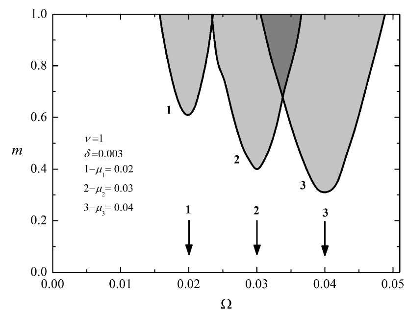
Figure 1: Regions of parameters wherein the excitation of high-frequency oscillations take place (gray).

The time evolution of the oscillations in the system is illustrated in Fig. 2. for the parameters of Fig 1, $\Omega$=0.04 and $m=$0.6. The intensity of the excited oscillations increases exponentially. There is no saturation of the intensity since(1) does not account for a particular nonlinearity that can be responsible for the intensity saturation. Dissipative nonlinearity, anharmonizm of the oscillators, or limiting power of the pumping oscillator can lead to a saturation of the intensity in a practical implementation of such generator.

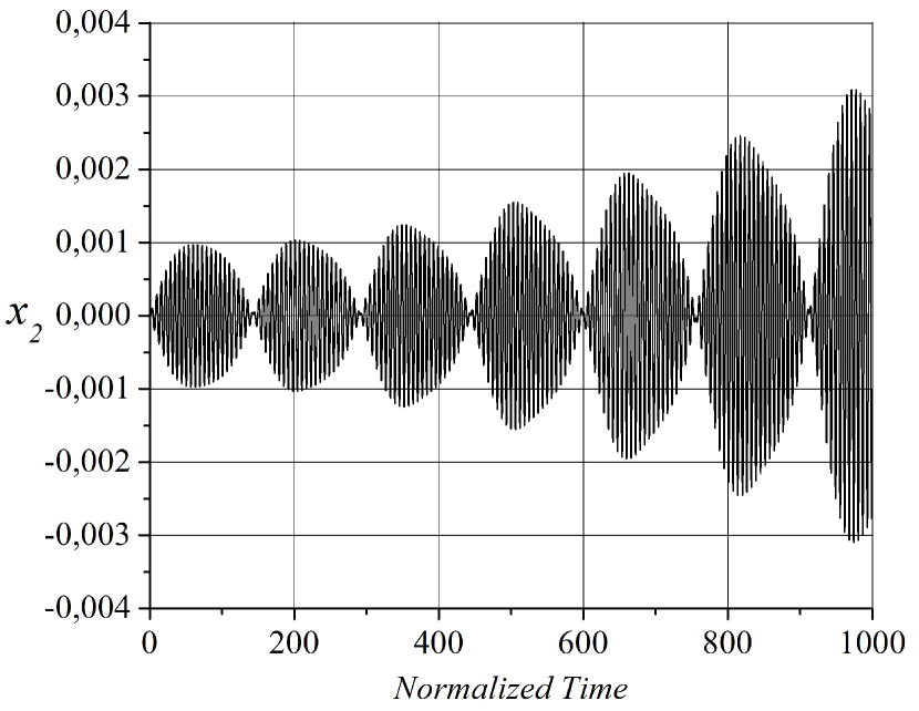
Figure 2: Build-up of the oscillation.

From Fig. 2, we note that the excited oscillation is modulated. This modulation take places at the frequency $\Delta\omega$. This is the manifestation of the fact that a two-frequency oscillation is simultaneously excited with the frequencies close to the natural frequencies $\omega_{1}$ and $\omega_{2}$. Since $\left|{\omega_{1}-\omega_{2}}\right|<<\omega_{1},\omega_{2}$, the superposition of the oscillations results in the observed modulation (beating).

III EXPERIMENT

For the first demonstration of the feasibility of the proposed generation mechanism we used two coupled RLC-oscillators as shown in Fig. 3. The partial frequencies of the oscillators were equal to 19.935 MHz, and the Q-factors of the unloaded first and second oscillators were 200 and 220, respectively. A coupling between the first (L1, C1) and the second (L2,C2)

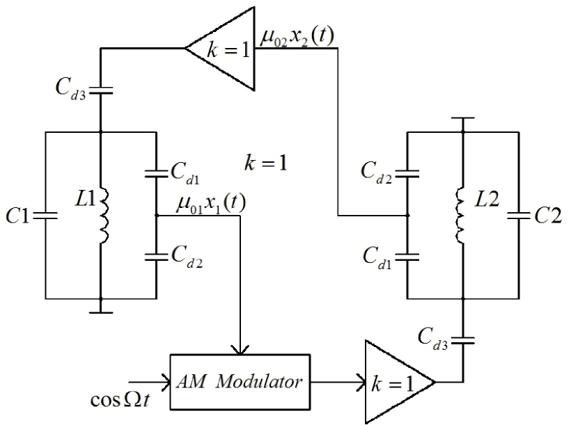
Figure 3: Circuit diagram of the generator.

oscillators is provided by using a capacitor coupler (Cd1, Cd2, Cd3), a buffer circuit and a modulator. The buffer circuit, implemented using IC AD8009, acts as an isolator providing the transfer coefficient is equal to 0 dB and -20 dB in the forward and reverse direction, respectively. The modulator, based on the FET BF998, is introduced to provide the modulation of the coupling coefficient. The modulator is driven by an external low-frequency oscillator.

The coupling from the second to the first oscillator is provided in the same manner, but the modulator is not introduced here.

We measured the natural frequencies of the coupled oscillators when the modulation was not applied. These frequencies are 19.656 MHz and 20.214 MHz. For symmetrical and constant coupling ($\mu_{01}=\mu_{02}\equiv\mu_{0})$ and for the indicated value of $\nu$ it gives $\mu_{0}/v^{2}$=0.29. Such value of the coupling coefficients follows also from the characteristics of the capacitor dividers used in the experimental set up in Fig. 3.

An example of a comparison of the experimental and theoretical bifurcation diagrams is given in Fig. 4. In the experiment, the minimum modulation coefficient for the generation onset is reached at the modulation frequency of about 0.58MHz, which is rather close to the measured value of $\Delta\omega$.

A typical waveform and the spectrum of the output oscillation is shown on Fig. 5 and Fig. 6, respectively. There are two intensive spectral components in the spectrum at the frequencies that are rather close to the natural frequencies indicated above. The superposition of such harmonic components results in the modulation of the output oscillation envelope as it is seen from Fig. 6. The output power in our experiment is limited by the power of the low-frequency oscillator used for the pumping.

From our point of view, the experimental results completely confirm the results following from the presented theoretical study.

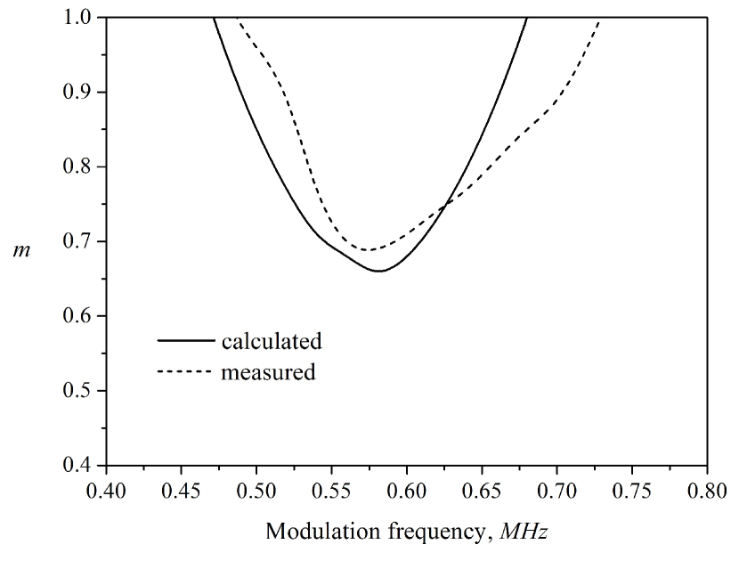
Figure 4: Calculated and measured boundaries of the arias, where the excitation of the oscillation takes place.

Figure 5: Waveform of the excited oscillation.

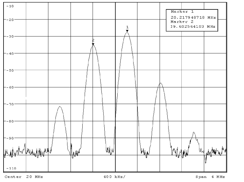
Figure 6: Spectrum of the excited oscillation.

IV DISCUSSION AND CONCLUSION

The described mechanism of the generation of high-frequency oscillations can be explained by using an energy diagram shown in Fig. 7. There are two energy levels $\hslash\omega_{1}$ and $\hslash\omega_{2}$ that are determined

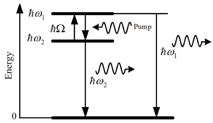
Figure 7: Diagram of the generation in the pumped coupled oscillators.

by the natural frequencies of the coupled oscillators. The width of the levels are respectively $\hslash\omega_{1}/Q_{1}$ and $\hslash\omega_{2}/Q_{2}$, where $Q_{1}$ and $Q_{2}$ are quality factors of the oscillators. When pumping with the energy $\hslash\Omega$ is applied, the transition

$$\hslash\omega_{2}+\hslash\Omega\rightarrow\hslash\omega_{1}$$ (15)

occurs leading to increasing the population of the higher-lying level. Next, since there is a coupling between the higher-lying and the lower-lying level, the transition

$$\hslash\omega_{1}\rightarrow\hslash\omega_{2}$$ (16)

also takes place. This process is accompanied by the radiation on the frequency $\omega_{1}-\omega_{2}$. But the most important is that due to (1), a feedback is realized in the system. This feedback is the condition to realize a self-excitation of high-frequency oscillations.

Next, since the coupling between the oscillators is not reciprocal, there is always a population inversion of the levels necessary for the development of the processes (15) and (16). The population of the levels is saturated due to a nonlinear effect.

When a load is connected, the system oscillates at the frequencies $\omega_{1}$, $\omega_{2}$, and their combinations, what is also seen from the spectrum of output oscillation in Fig. 6.

We have experimentally demonstrated the suggested excitation mechanism by using conventional lamped electronic components. It allows us to excite oscillations at the frequencies around 20 MHz by the external pumping at the frequency of 0.58 MHz. Such realization is convenient from the point of view of reliable and detailed comparison of the experimental data and the theoretical results. The proposed method for generating electromagnetic oscillations is very simple since it does not require sophisticated nonlinear elements or media for its realization. Therefore, this mechanism is especially interesting for the development of generators for much higher frequencies. For example, the availability of high-Q THz resonators [9] and variety of Ka-band oscillators available for the pumping and modulators create a solid background for the development of THz generators based on the proposed approach.

References

- Lichtenberg and Lieberman (1983) A. J. Lichtenberg and M. A. Lieberman, Regular and stochastic motion (Springer-Verlag New York Heidelberg Berlin, 1983) p. 499.
- Nayfeh et al. (1994) A. H. Nayfeh, S. A. Nayfeh, and B. Balachandran, “Transfer of energy from high-frequency to low frequency modes,” in Nonlinearity and Chaos in Engineering Dynamics, edited by J. M. T. Thompson and S. R. Bishop (John Wiley and Sons Ltd, 1994) pp. 39–58.
- Oksasoglu and Vavriv (1994) A. Oksasoglu and D. M. Vavriv, IEEE Trans. Circuits and Systems. 41, 669 (1994).
- Vavriv et al. (1996) D. M. Vavriv, V. B. Ryabov, S. A. Sharapov, and H. M. Ito, Physical Review E 53, 103 (1996).
- Shygimaga et al. (1998) D. V. Shygimaga, D. M. Vavriv, and V. Vinogradov, IEEE Trans. Circuits and Systems 45, 1255 (1998).
- Buts (2001) V. A. Buts, Problems of Atomic Science and Technology. Special issue dedicated to the 90-th birthday anniversary of A.I. Akhiezer. 6, 329 (2001).
- Buts (2004) V. A. Buts, Electromagnetic waves and electron systems (In Russian) 9, 59 (2004).
- Bogoliubov and Mitropolski (1961) N. N. Bogoliubov and Y. A. Mitropolski, Asymptotic Methods in the Theory of Nonlinear Oscillations (Gordon and Breach, New York, 1961).
- Yang et al. (2012) B. B. Yang, S. L. Katz, K. J. Willis, M. J. Weber, I. Knezevic, S. C. Hagness, and J. H. Booske, IEEE Trans. THz Science and Technology 2, 449 (2012).