Multivariate regression and fit function uncertainty

Abstract

This article describes a multivariate polynomial regression method where the uncertainty of the input parameters are approximated with Gaussian distributions, derived from the central limit theorem for large weighted sums, directly from the training sample. The estimated uncertainties can be propagated into the optimal fit function, as an alternative to the statistical bootstrap method. This uncertainty can be propagated further into a loss function like quantity, with which it is possible to calculate the expected loss function, and allows to select the optimal polynomial degree with statistical significance. Combined with simple phase space splitting methods, it is possible to model most features of the training data even with low degree polynomials or constants.

1 Introduction

Regression methods are frequently used in particle physics, usually to quantify a continuous curve or surface that simplifies statistical sample. Typical examples are the calibration curves for certain detector responses and neural networks trained to identify particle. The mathematical goal is finding a $f:x\rightarrow y$ map between the $x$ input space to the $y$ target space in such a way that $f(x)$ predicts the $\mathbb{E}(y|x)$ conditional expectation value with statistical certainty. The least squares algorithm is known to converge to the conditional mean, given it is a finite number and the parametric $f$ function is in the family that contains the solution. This latter information is not always given and one must chose a function family general enough to cover unexpected features. Such a function family are the logistic functions and the radial base functions and generally the kernels. For these one usually has to determine an ideal degree of freedom for the fit, namely the number of base functions to be used in order to avoid overtraining of the data and so avoiding picking up non-significant features from the statistical fluctuation. Although these are straightforward procedures, it is computationally intensive to find the global minimum of the sum of squares for the fit. A usually unexploited feature of the least squares method is that the global minimum can be exactly determined for kernels with fixed position in the $x$ space, because the amplitude that minimizes the sum of squares can be calculated with a linear equation, without numerical optimization.

With given $k_{i}(x),i\in{1..n_{d}}$ kernels and $a_{i}$ amplitudes the sum of squares for the data points $\{x_{j},y_{j}\},j\in\{1..N\}$ will take the form

$$E_{\chi^{2}}=\frac{1}{N}\sum_{j}\left(y_{j}-\sum_{i}a_{i}k_{i}\left(x_{j}\right)\right)^{2}=\langle y^{2}\rangle-\sum_{i}2a_{i}\langle yk_{i}(x)\rangle+\sum_{il}a_{i}a_{l}\langle k_{i}(x)k_{l}(x)\rangle\,,$$ (1)

where the angled brackets $\langle\rangle$ indicate averaging over the sample. The loss function $E_{\chi^{2}}$ in eq. (1) can be minimised in respect of the $f_{i}$ amplitudes with

$$f_{i}=\sum_{l}G_{il}^{-1}h_{l}$$ (2)

by using the matrix $G_{il}=\langle k_{i}(x)k_{l}(x)\rangle$ and the vector $h_{i}=\langle yk_{i}\rangle$. The $G_{il}$ matrix is symmetric and has $\frac{1}{2}n_{d}(n_{d}-1)$ parameters. A possible way to decrease the number of parameters is to use kernels which are power series $k_{i}(x)=k_{1}^{i}(x)$, resulting in a Hankel-type matrix $G_{il}=\langle k_{1}(x)^{i+l}\rangle$. A simple power series kernel might be based on the monomials, $k_{1}(x)=x,k_{i}(x)=x^{i}$, resulting in polynomial fitting. An other advantage of fitting a fix degree polynomial instead of Gaussian or a sigmoid kernels is that polynomials are not sensitive to the shift of features in the data, in other words they are translation invariant.

2 Uncertainty and covariance of large weighted random sums

The advantage of using matrix formalism in eq. (1) is that the original training data $\{x_{j},y_{j}\}$ is compressed into the $h_{i}$ vector and the $G_{il}$ matrix, which can be a great reduction in the number of input parameters. These input parameters are themselves random variables having a certain distribution that in principle could be derived from the generating distribution of the $\{x_{j},y_{j}\}$ sample and the number of measurements $N$. Due to the central limit theorem, the generating distribution itself is not need to be known, only that it fulfils certain criteria, since $h_{i}$ and $G_{il}$ are generated by summing up random variables. Probably the most widely known of the central limit theorems is the one stating that if the generating distribution of the $X_{i},i\in\{1..N\}$ random variables has finite mean $\bar{X}$ and variance $\sigma_{X}$, then the distribution of the variable $s=\frac{1}{\sigma_{X}}(\sum_{i}X_{i}/N-\bar{X})$ converges to the normal distribution.

The approximation of the covariance matrix of the $p_{m}=(h_{1},...,h_{n_{d}},g_{1},...,g_{2{n_{d}}}),m\in\{1,...,3{n_{d}}\}$ input parameters for polynomial regression is the following. In a general formalism, every data point with index $j$ are triplets, consisting of an input value $x_{j}$, a target value $y_{j}$ and a weight $w_{j}$. With $b\in\{0,1\}$, $k_{0}\{1,...,{n_{d}}\}$, $k_{1}\in\{1,...,2{n_{d}}\}$ the input parameter with pseudo index $m={k_{b}+b{n_{d}}}$ is calculated as

$$p_{m}=\frac{1}{\sum_{j}w_{j}}\sum_{j}w_{j}y_{j}^{b}x_{j}^{k_{b}}\,.$$

The product $a_{j}=w_{j}y_{j}^{b}x_{j}^{k_{b}}$ for each $i$ index can be treated as a compound random variable. The $\nicefrac{{1}}{{\sum_{j}w_{j}}}$ was not introduced into this new variable, because that would ruin the independence. Let’s define the following variables in order to estimate the probability distribution of $p_{m}$ . Let $\langle aw\rangle=\frac{1}{N}\sum_{j}w_{j}a_{j}$ be the weighted average of $a_{j}$. This is approximately a Gaussian variable with mean $\langle aw\rangle$ and variance $\sigma^{2}_{\langle aw\rangle}=\frac{1}{N(N-1)}\sum_{j}{(a_{j}w_{j}-\langle aw\rangle)^{2}}$. Define the average weight similarly as $\langle w\rangle=\frac{1}{N}\sum_{j}w_{j}$, which is also distributed as a Gaussian with mean $\langle w\rangle$ and variance $\sigma^{2}_{\langle w\rangle}=\frac{1}{N(N-1)}\sum_{j}{(w_{j}-\langle w\rangle)^{2}}$. These variables are indeed correlated, and their covariance is $\text{Cov}\left(\langle aw\rangle,\langle w\rangle\right)=\frac{1}{N(N-1)}\sum_{j}{(a_{j}w_{j}-\langle aw\rangle)(w_{j}-\langle w\rangle)}$. The above definitions show, that $p_{m}$ is a ratio of two Gaussian variables. Its expectation value is $p_{m}$, while its variance can be approximated with error propagation. Assuming that $\sigma_{\langle w\rangle}/\langle w\rangle\gg 0$, the approximation of the variance of $p_{m}$ is

$$\sigma_{p_{m}}^{2} =\begin{pmatrix}\frac{\partial p_{m}}{\partial\langle aw\rangle}\\[3.00003pt] \frac{\partial p_{m}}{\partial\langle w\rangle}\end{pmatrix}^{\text{T}}\begin{pmatrix}\sigma^{2}_{\langle aw\rangle}&\text{Cov}\left(\langle aw\rangle,\langle w\rangle\right)\\ \text{Cov}\left(\langle aw\rangle,\langle w\rangle\right)&\sigma^{2}_{\langle w\rangle}\end{pmatrix}\begin{pmatrix}\frac{\partial p_{m}}{\partial\langle aw\rangle}\\[3.00003pt] \frac{\partial p_{m}}{\partial\langle w\rangle}\end{pmatrix}$$

$$=\dfrac{1}{\langle w\rangle^{2}}\sigma_{\langle aw\rangle}^{2}+\dfrac{\langle aw\rangle^{2}}{\langle w\rangle^{4}}\sigma_{\langle w\rangle}^{2}-2\dfrac{\langle aw\rangle}{\langle w\rangle^{3}}\text{Cov}\left(\langle aw\rangle,\langle w\rangle\right)$$ (3)

$$=\dfrac{1}{\langle w\rangle^{2}}\sum_{j}\dfrac{w_{j}^{2}(\langle aw\rangle-a_{j})^{2}}{N(N-1)}\,.$$ (4)

It can be seen that eq. (4) gives back the known formula for the standard deviation of $\langle a\rangle$ when all weights are $w_{j}=1$, which is also true when the weights are independent of the distribution of $a$. Similar derivation shows that the covariance between variables $p_{m_{1}}$ and $p_{m_{2}}$, with pseudoindices $m_{1}={k_{b_{1}}+b_{1}{n_{d}}}$ and $m_{2}={k_{b_{2}}+b_{2}{n_{d}}}$ can be calculated as

$$\text{Cov}\left(p_{m_{1}},p_{m_{2}}\right)=\dfrac{1}{\langle w\rangle^{2}}\sum_{j}\dfrac{w_{j}^{2}(\langle wy^{b_{1}}x^{k_{b_{1}}}\rangle-y_{j}^{b_{1}}x_{j}^{k_{b_{1}}})(\langle wy^{b_{2}}x^{k_{b_{2}}}\rangle-y_{j}^{b_{2}}x_{j}^{k_{b_{2}}})}{N(N-1)}\,.$$ (5)

The covariance and the variance estimation can be generalized to non-monomial kernels, by replacing $x^{k}$ in the above equations with the given kernel.

It must be noted that traditionally the uncertainty estimates on the fit parameters have different formulas. In most cases the sample $\{x_{j},y_{j}\}$ is augmented with the uncertainty of the target, the conditional variance in the $y$ direction, $\sigma_{y_{j}}^{2}$, which can be considered as prior knowledge. In that case the data points in the formation of the estimation of expectation values receive a $\sigma_{y_{j}}^{-2}$ weight and a $c=\sum_{j}\sigma_{y_{j}}^{-2}$ normalization factor. This choice of weight comes from the principle that the different measurements should be combined in a way that minimizes the uncertainty of the result, in this case the estimation of the expectation values. An example could be the $F(x)=a+bx$ least squares regression with $a,b$ unknowns on the $\{x_{j},y_{j},\sigma_{y_{j}}^{2}\}$ sample. The input parameters to this fit are

$$c=\sum_{j}\frac{1}{\sigma_{y_{j}}^{2}}\,,h_{0}=\langle y\rangle=\frac{1}{c}\sum_{j}\frac{y_{j}}{\sigma_{y_{j}}^{2}}\,,h_{1}=\langle yx\rangle=\frac{1}{c}\sum_{j}\frac{y_{j}x_{j}}{\sigma_{y_{j}}^{2}}$$

$$g_{0}=\langle x^{0}\rangle=1\,,g_{1}=\langle x\rangle=\frac{1}{c}\sum_{j}\frac{x_{j}}{\sigma_{y_{j}}^{2}}\,,g_{2}=\langle x^{2}\rangle=\frac{1}{c}\sum_{j}\frac{x_{j}^{2}}{\sigma_{y_{j}}^{2}}\,.$$

The optimal fit parameters are

$$\begin{pmatrix}a\\ b\end{pmatrix}=\begin{pmatrix}g_{0}&g_{1}\\ g_{1}&g_{2}\end{pmatrix}^{-1}\begin{pmatrix}h_{0}\\ h_{1}\end{pmatrix}$$

As $a$ and $b$ are linear functions of $y_{j}$, it is easy to calculate the expectation values needed for the covariance matrix:

$$\text{Cov}\left(a,b\right)=\mathbb{E}(ab)-\mathbb{E}(a)\mathbb{E}(b)=\frac{1}{c}\sum_{j}\frac{\partial a}{\partial y_{j}}\frac{\partial a}{\partial y_{j}}\sigma_{y_{i}}^{2}=\langle x\rangle=g_{1}\,.$$ (6)

Similarly, $\text{Cov}\left(a,a\right)=\sigma_{a}^{2}=g_{0}$ and $\text{Cov}\left(b,b\right)=\sigma_{b}^{2}=g_{2}$. This covariance matrix indeed differ from the one derived in eq. (5). The origin of the difference relies in the prior information that was built into the equations. In the case of eq. (5) the weights were provided with the data points, while in the case of eq. (6) the $\sigma_{y_{i}}^{2}$ was given – knowledge of the uncertainty on the $\mathbb{E}(y|x)$ conditional mean. The weights in the former case may come from Monte Carlo integration techniques or from weighted sample separation and it is thought to be fundamentally fixed, while in the latter case it is derived from the principle of optimal data combination. Though it is unclear whether the two methods could be combined, but the former method is thought to be superior as it was designed to approximate the $\sigma_{y(x)}^{2}$ from the sample itself, and also takes into account the uncertainty in the sampling of the input space $x$. Furthermore, it handles negative and zero weights correctly.

3 Fit function uncertainty

With the knowledge of the uncertainty of the input parameters $p_{m}=(h_{1},...,h_{n_{d}},g_{1},...,g_{2{n_{d}}}),m\in\{1,...,3{n_{d}}\}$, one can estimate the uncertainty of the fitted kernel amplitudes using linear error propagation in eq. (2). The first derivatives of $f_{j}=\sum_{l}G_{il}^{-1}h_{l},G_{il}=g_{i+l}$ are

$$\frac{\partial f_{i}}{\partial\langle h_{l}\rangle}=G_{il}^{-1}$$

$$\frac{\partial f_{i}}{\partial\langle g_{o}\rangle}=-\sum_{lmn}G_{im}^{-1}\frac{\partial G_{mn}}{\partial{g_{o}}}G_{nl}^{-1}h_{l}\,.$$

Together with the previously calculated covariace matrix, the uncertainty of the fit function $F(x)=\sum_{i}f_{i}x^{i}$ at a given $x$ point is

$$\sigma^{2}_{F(x)}=\sum_{nm}\frac{\partial\sum_{i}f_{i}x^{i}}{\partial p_{m}}\text{Cov}\left(p_{m},p_{n}\right)\frac{\partial\sum_{l}f_{l}x^{l}}{\partial p_{n}}\,.$$

The uncertainty of the fitted function does not necessarily cover the true $\mathbb{E}(y|x)$ conditional mean. That only happens if the fit function is general enough to discover all the features of the sample. The meaning of this uncertainty is deeply routed in the central limit theorem. When the central limit theorem was applied to the $p_{m}$ input parameters, only the fact that the distribution of certain sums can be modeled with a Gaussian distribution came from the theorem, the width and the mean of this Gaussian came from a maximum likelihood fit. This is typically interpreted as a posterior distribution for the true mean, but it can also be interpreted as a model fitted to the sample and predicting where the sum may converge with additional data points. The same can be said about the Gaussian uncertainty of the fit function. It tells us the likelihood where the fit function with the same degrees of freedom would converge with additional data, and not the position of the conditional mean. This is why some methodology is needed to compare fit functions with different degrees of freedom and see if the sample can be described better with one or the oter.

4 The uncertainty of the loss function

In the case of polynomial fitting one has to determine the degree of polynomial that is still statistically meaningful. Using too many degrees of freedom in a fit can result in overfitting or eventually in interpolation of the data points. In the latter case the $E_{\chi^{2}}$ loss function simply reaches its absolute minimum, zero. However, the uncertainty of the fitted function increases with the number of degrees of freedom and this can be exploited in order to select significant features only, though one has to keep in mind that the Gaussian approximation of the distribution of the $p_{m}$ input parameters has a limitation. First, the Gaussian approximation is only true if the number of input points $N$ is large enough. Second, the uncertainty of the estimated covariance matrix may also increase to be comparable with the covariance matrix itself if the number of degrees of freedom in the fit is comparable to the number of sample points.

The naïve way of comparing the optimized $F^{\text{opt}}_{d_{1}}(x)=\sum_{ik}^{d_{1}}h_{i}G_{d_{1},ik}^{-1}x^{k}$ with degrees of freedom $d_{1}$ to $F^{\text{opt}}_{d_{2}}(x)$ with degrees of freedom $d_{2}$ would be calculating their loss functions $E_{d_{1},\chi^{2}}=\frac{1}{N}\sum_{j}(y_{i}-F^{\text{opt}}_{d_{1}}(x))^{2}$ and $E_{d_{2},\chi^{2}}$ and checking whether their difference is significantly different then zero. This procedure does not work, as the approximate distribution of $E_{d_{1},\chi^{2}}$ is not a good measure of fitness after the $F^{\text{opt}}_{d_{1}}(x)$ is substituted. It can be seen on an example where the $x$ space is thought to be non-random and only the $y$ coordinates of the sample points might vary when a new sample is obtained. After the substitution of $F^{\text{opt}}_{d}(x)$ into $E_{d,\chi^{2}}$ it can be simplified to

$$E_{d,\chi^{2}} =\langle y^{2}\rangle-2\sum_{i}F^{\text{opt}}_{d,i}h_{i}+\sum_{ik}F^{\text{opt}}_{d,i}G_{ik}F^{\text{opt}}_{d,k}$$

$$=\langle y^{2}\rangle-\sum_{ik}h_{i}G_{ik}^{-1}h_{j}\,,$$

which has an approximate expectation value

$$\mathbb{E}(E_{d,\chi^{2}}) =\langle y^{2}\rangle-\mathbb{E}(\sum_{ik}h_{i}G_{ik}^{-1}h_{j})$$

$$=\langle y^{2}\rangle-\sum_{ik}h_{i}G_{ik}^{-1}h_{j}-\sum_{ik}G_{ik}\text{Cov}\left(h_{i},h_{k}\right)\,.$$

It contains a bias term compared to $E_{d,\chi^{2}}$ and allows $\mathbb{E}(E_{d,\chi^{2}})$ to be lower than $E_{d,\chi^{2}}$. This bias means that the approximate distribution of $E_{d,\chi^{2}}$ is not related to the goodness of fit anymore, but to the possible $E_{d,\chi^{2}}$ minima.

Ideally, the best measure of fitness would be a distance-like variable between the fit function and the real $\mathbb{E}(y|x)$ conditional expectation value. A good approximation to that is of course the loss function applied to $F^{\text{opt}}_{d}(x)$, but one must differentiate it from the previously described $E_{d,\chi^{2}}$. In this picture, one must treat the sample as an approximation to $\mathbb{E}(y|x)$, and not as a random variable. Let’s call it the cross validation loss function, where only the $F^{\text{opt}}_{d}(x)$ is a random variable:

$$E_{d,\chi^{2}}^{+}=\underbrace{\langle y^{2}\rangle}_{\text{fixed}}-2\sum_{i}\underbrace{F^{\text{opt}}_{d,i}}_{\text{varied}}\underbrace{h_{i}}_{\text{fixed}}+\sum_{ik}\underbrace{F^{\text{opt}}_{d,i}}_{\text{varied}}\underbrace{G_{ik}}_{\text{fixed}}\underbrace{F^{\text{opt}}_{d,k}}_{\text{varied}}\,.$$

As the first derivative of $\frac{\partial E_{d,\chi^{2}}^{+}}{\partial p_{m}^{\prime}}=0$ at $p_{m}^{\prime}=\mathbb{E}(p_{m})$, the expectation value of $E_{d,\chi^{2}}^{+}$ can be approximated through its second derivative as

$$\mathbb{E}(E_{d,\chi^{2}}^{+}) =\langle y^{2}\rangle-2\sum_{i}h_{i}\mathbb{E}(F^{\text{opt}}_{d,i})+\sum_{ik}G_{ik}\mathbb{E}(F^{\text{opt}}_{d,i}F^{\text{opt}}_{d,k})$$

$$=E_{d,\chi^{2}}^{+}+\frac{1}{2}\sum_{lm}\frac{\partial^{2}E_{d,\chi^{2}}^{+}}{\partial p_{m}\partial p_{l}}\text{Cov}\left(p_{m},p_{l}\right)\,,$$ (7)

where the second derivative of $E_{d,\chi^{2}}^{+}$ was taken at the expectation values of $p_{m}$, and can be expressed as a block matrix

$$\frac{\partial^{2}E_{d,\chi^{2}}^{+}}{\partial p_{m}\partial p_{l}}=\begin{pmatrix}2G_{lm}^{-1}&-4\sum_{kno}G_{lk}^{-1}\frac{\partial G_{k}n}{\partial p_{m}}G_{no}^{-1}h_{o}\\[6.00006pt] -4\sum_{kno}G_{mk}^{-1}\frac{\partial G_{k}n}{\partial p_{l}}G_{no}^{-1}h_{o}&6\sum_{knowrqp}h_{k}G_{ko}^{-1}\frac{\partial G_{o}w}{\partial p_{l}}G_{wr}^{-1}\frac{\partial G_{r}p}{\partial p_{m}}G_{pq}^{-1}h_{q}\end{pmatrix}$$

Since in $E_{d,\chi^{2}}^{+}$ is a quadratic formula and only the fit function is varied, its expectation value can not be lower than the minimum taken at $F^{\text{opt}}_{d}(x)$ by construction. In most cases the second degree Taylor polynomial approximation in eq. (7) in the $p_{m}$ variables is enough as it is quadratic in the $h_{i}$ and the dependence on the $G^{-1}_{ik}$ is usually weak, because $G_{ik}$ depends on the sampling in $x$ and does not affect the $\mathbb{E}(y|x)$ conditional expectation value in the large sample size limit. Therefore for large sample sizes and approximately error-free $G_{ik}$ matrices $\frac{\partial^{2}E_{d,\chi^{2}}^{+}}{\partial p_{m}\partial p_{l}}$ can be approximated with the its upper left submatrix, that represents the derivatives of $h_{l}$ and $h_{m}$. In this approximation $E_{d,\chi^{2}}^{+}$ is a $\chi^{2}$ variable with $d$ degrees of freedom, given that the covariance matrix $\text{Cov}\left(h_{i},h_{k}\right)$ is non-singular.

In the full calculation of the standard deviaton of $E_{d,\chi^{2}}^{+}$ one should include the variable $\langle y^{2}\rangle$ and its correlation to the other input parameters $p_{m}$. Nevertheless, the $\langle y^{2}\rangle$ term disappears when a loss function difference is calculated for two different fit functions, and it can be shown that the variance of the loss function differences can be calculated solely from the variance of the individual $E_{d,\chi^{2}}^{+}$ terms, neglecting the contributions from $\langle y^{2}\rangle$. This type of variance is twice the square of the previously described bias term in the expectation value in eq. (7), as it would be exptected for a $\chi^{2}$ distribution:

$$\sigma^{2}_{d,E^{+}}=2\left(\frac{1}{2}\sum_{lm}\frac{\partial^{2}E_{d,\chi^{2}}^{+}}{\partial p_{m}\partial p_{l}}\text{Cov}\left(p_{m},p_{l}\right)\right)^{2}\,.$$

Similar to the behaviour of $\chi^{2}$ differences, the expectation value of the $E_{d2,\chi^{2}}^{+}-E_{d1,\chi^{2}}^{+}$ difference is the difference of their expectation values. The same can be said about the variance of $E_{d2,\chi^{2}}^{+}-E_{d1,\chi^{2}}^{+}$, as it can be calcuated from the square root of the individual $E_{d2,\chi^{2}}^{+}$ variations:

$$\sigma_{d_{1},d_{2},\Delta E^{+}}=|\sigma_{d_{2},E^{+}}-\sigma_{d_{1},E^{+}}|\,.$$

This addition rule makes it extremely simple to find the optimal degrees of freedom $d$, as there is no need to calculate covariance matrices belonging to the different fit functions. This makes the significance of a feature not only relatively true, but absolute. To optimize the degree of freedom $d$ with a certain significance level, it is enough to minimize $\mathbb{E}(E_{d,\chi^{2}}^{+})+s\sigma_{d,E^{+}}$, where $s$ can be arbitrarily chosen. Due to the characteristics of the $\chi^{2}$ distribution, optimizing for the minimal expected $E_{d,\chi^{2}}^{+}$ results in selecting features that are at least $50\%$ significant.

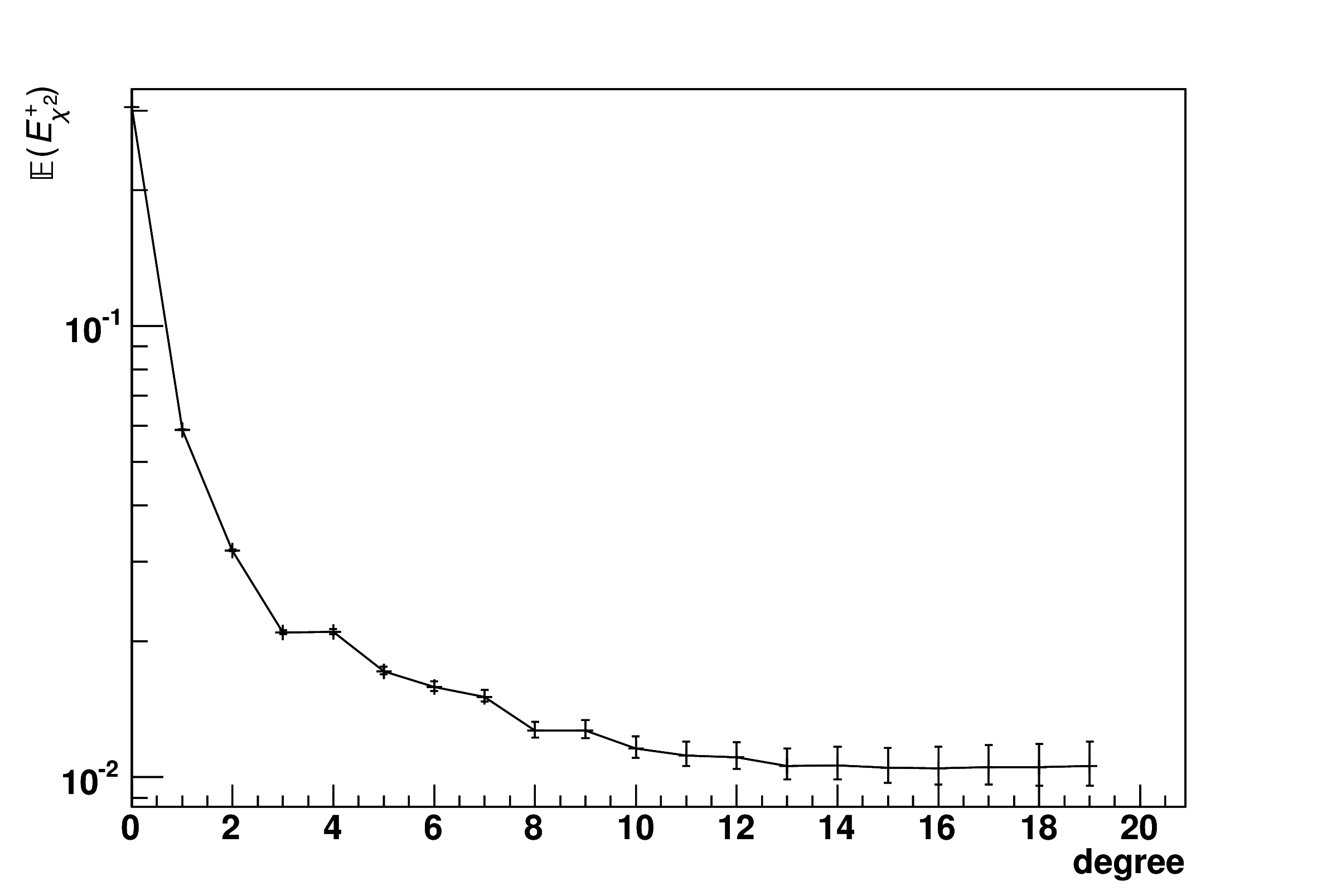
(a) dependence of the expected loss function on the degrees of freedom

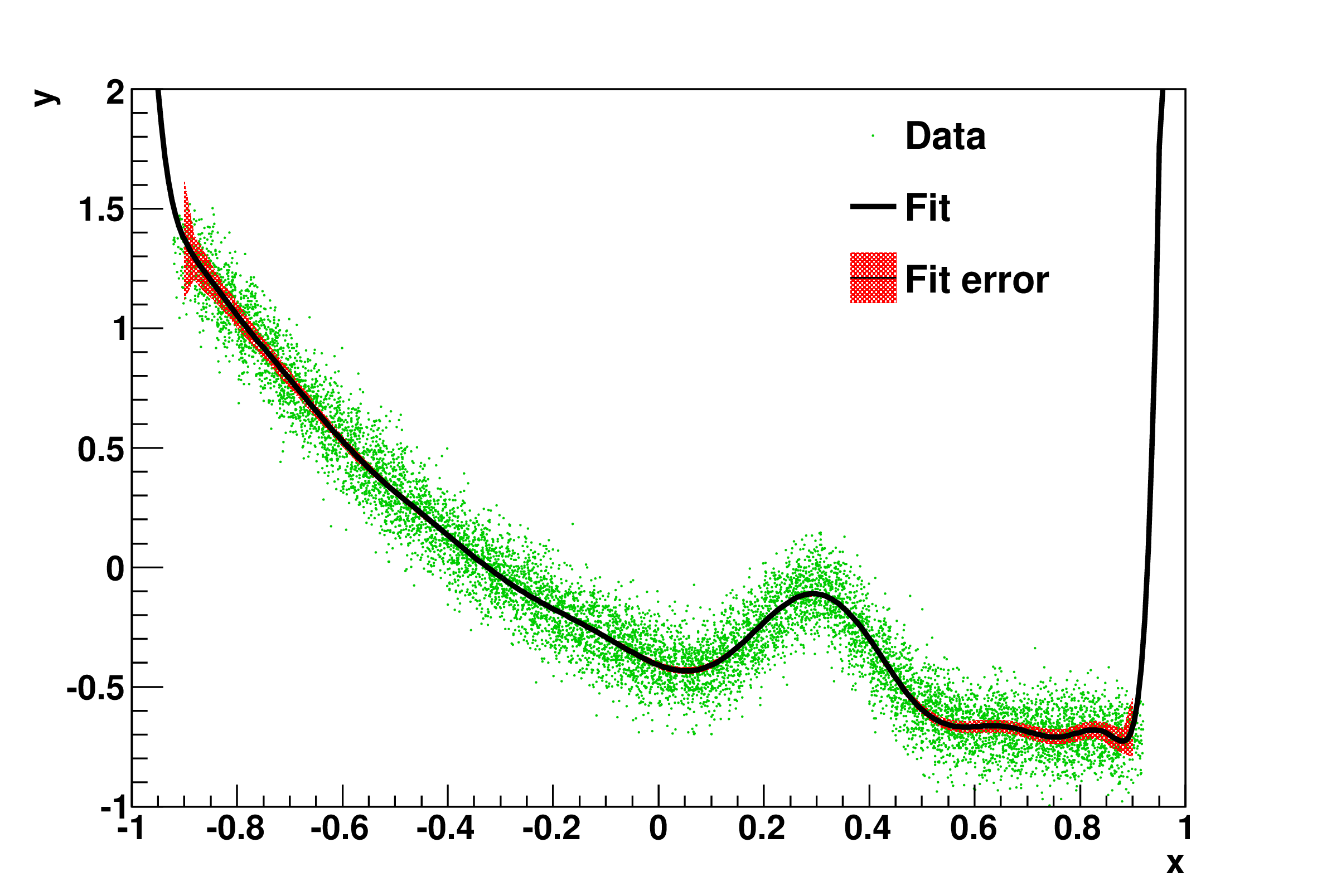
(b) regression with a single 16 degree polynomial

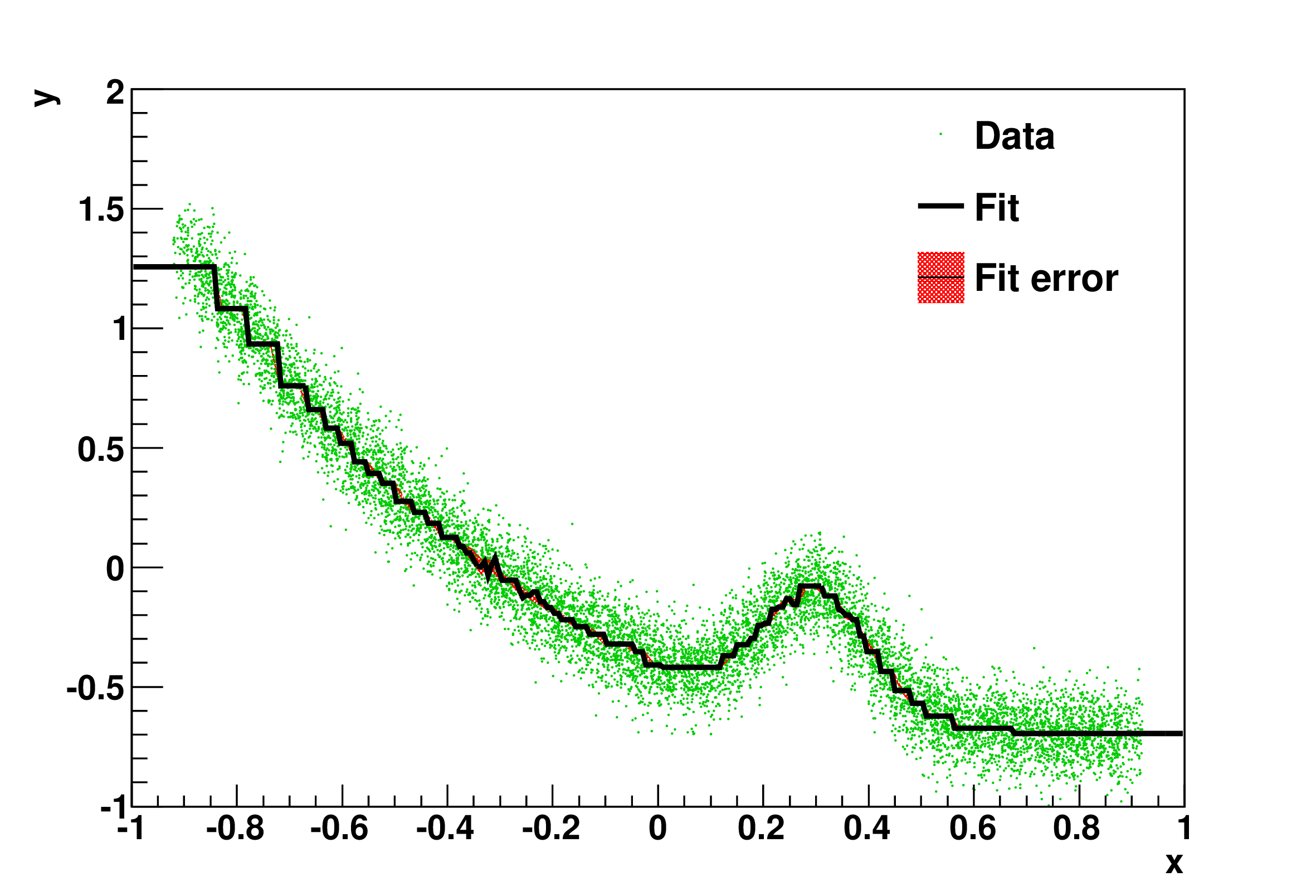
(c) regression with constants

(d) regression with linear functions

Figure 1: Example univariate regression. The training sample was a uniform distribution in $x\in(-0.9,0.9)$ and a Guassian smearing in the y direction for every $x$. The expected loss function in fig. 1a has a minimum for the 16 degree polynomial. The bottom of the error bar represents the $E_{d,\chi^{2}}$ loss function evaluated with the optimal polynomial, the data points are the $\mathbb{E}{(E_{d,\chi^{2}}^{+})}$ expectation values, while the upper error bars show the one standard deviations of $E_{d,\chi^{2}}^{+}$ above the expectation value. Figure 1b shows the 16 degree optimal polynomial with very large uncertainties at the two edge of the sample. Figure 1c and 1d shows regressing with a splitting procedure described in the bulk of the text, with allowed maximal polynomial degrees $n_{\text{max}}=0$ and $1$ accordingly. Both of these regressions functions are within one sigma of the conditional $\mathrm{P}(y|x)$ distribution and approximates the $\mathbb{E}(y|x)$ conditional expectation value without picking up statistical noise.

5 Determining the right polynomial order

Selecting the right modelling function can be understood as a repeated hypothesis testing. One must decide a priori about the null hypothesis and the series of hypotheses to test. In case of polynomial fitting, the ordering seems trivial, going from a constant to higher polynomial orders. However, with multivariate input $x_{\mu}$, a polynomial can be defined with a different degree belonging to each $\mu$ index. In this case, one may still choose a common order, as the optimizing method described in the previous section allows the comparison of fit functions differing in multiple degrees of freedom. A common polynomial order is special in the sense that it is closed under the group of rotations and translations, treating the different $\mu$ directions equally.

However, it is not possible to compare the loss functions of the infinite many polynomials. Not only because it is infeasible, but alse because one must stop before the numerical errors overcome the estimated uncertainties in $E^{+}_{\chi^{2}}$. It is not straightforward to estimate these numerical errors, but as a guideline it can be said that it increases with both the number of polynomial degrees and the number of input dimensions in the multivariate case. The polynomial degree necessitate an exponentiation on the input parameters, which both appears in the training and in the function evaluation phase. A double precision number can be thought of as a sixteen digit decimal number, and though its $n^{\text{th}}$ exponential is expected to have a relative error of only $n\cdot 10^{-16}$, the numerous subtractions and multiplications needed for the linear equation solver can easily blow this up. In the univariate case, it numerical errors seems to become significant at the polynomial order around 20 for double precision and $24...30$ for 128bit long double precision. In the case of $d$ input dimensions the size of the $G$ matrix grows rapidly with the degrees. It is because the polynomial coefficients of the $F(x)$ fit function are $d$-degree symmetric tensors, with $\binom{n+d-1}{n}$ free parameters, and all the free parameters in $F(x)$ contribute to the size of the $G$ matrix. For 20 input dimensions a 3 degree polynomial has nearly 2000 free parameters, resulting in $G$ matrix size of $2000\times 2000$, and although solving a linear equation with this only takes a few seconds on a modern-day computer, this also means that more than a million instructions are needed to express each unknown of the $F(x)$ polynomial, resulting in large numerical errors.

(a) original

(b) remodelled

Figure 2: Figure LABEL:sub@fig:originalArcher shows a photo of a Chinese terra-cotta soldier, whose intensity map was remodelled in fig. LABEL:sub@fig:remodelledArcher in small patches with polynomials. The photo was treated as a random sample, namely that prior knowledge of the uncertainty of the pixel intensities were neglected. The region boundaries were determined with algorithm described in the bulk of the text, based on the principal axes of the input distribution. The regions were modelled with a two dimensional linear polynomial, with a second layer of univariate regression upon it, to simulate a sigmoid-like behaviour. Over- and undershoots from the displayable range were rounded to the maximum and minimum intensities accordingly. A photo instead of a real 3D distribution was chosen here in order to demonstrate that this simple fitting and splitting method can detect the significant features in the data while smoothing the small details, as one would require for a regression method on a statistical sample.

6 Minimizing numerical errors

To overcome the problem of the high polynomial degrees and the large matrices, one can split the sample into many smaller phase spaces, which may require smaller polynomial degrees. For this one must decide on a maximal polynomial degree $n_{\text{max}}$ which is allowed in regression, and $n_{\text{max}}+k$, $k>1$ which up to expected loss function is scanned. If the optimal degree of the expected loss function appears to be larger than $n_{\text{max}}$, one can apply a predefined algorithm that splits the input phase space. One such algorithm for the univariate case simply splits the input phase space at the $x$ mean, as demonstrated on fig. 1. This requires practically no additional computation, since the $\langle x\rangle$ was already calculated for the regression. The splitting and fitting can be repeated until the full sample is regressed. A possible extension of this approach to the multivariate case finds the multivariate mean $\langle x_{\mu}\rangle$ first, then splits the sample at this point parallel to the principal axis, the eigenvector with the largest eigenvalue of the $\langle x_{\mu}x_{\nu}\rangle-\langle x_{\mu}\rangle\langle x_{\nu}\rangle$ matrix; see fig. 2. These methods have the advantage that they place the cut boundaries within the distribution, so the regression on these phase spaces are less likely to produce degenerate solutions. A seemingly more optimal splitting method would be finding the place where the fitted polynomial with $n_{\text{max}}+1$ degrees have the largest derivative, since this is a hard place to model with an $n_{\text{max}}$ degree polynomial. However, it is non-trivial to define and find this boundary in the multivariate case, and this boundary typically appear nearby the tails of the $x$ distribution, where the fitted function has the largest uncertainty.

7 Conclusions

The presented method is capable of modelling multivariate statistical data with polynomials by detecting the significant features in the data. It is a fast and robust method, as most calculations are computationally very simple and it does not require numerical optimisation. Similarly to the statistical bootstrap method, the uncertainty of the regression function can be determined from the training sample, but in this case analytically. In combination with a phase space splitting method, it can be extended to fit very complex data, still maintaining numerical stability.

References

References

- [1] Kövesárki P 2012 ArXiv e-prints 5 (Preprint 1203.5647)
- [2] Kövesárki P 2012 Multivariate methods and the search for single top-quark production in association with a W boson in ATLAS Ph.D. thesis University of Bonn URL {http://hss.ulb.uni-bonn.de/2013/3188/3188.htm}
- [3] Kövesárki P 2013 ACAT 2013 Beijing URL http://indico.ihep.ac.cn/conferenceOtherViews.py?view=standard&confId=2813
- [4] Metzger W J 2010 Statistical Methods in Data Analysis (Radboud Universiteit Nijmegen, The Netherlands) ISBN HEN-343 URL http://www.hef.ru.nl/~wes/stat_course/statist.pdf
- [5] The European Mathematical Society Encyclopedia of Mathematics 1 URL {http://www.encyclopediaofmath.org/index.php?title=Hankel_matrix&oldid=23850}
- [6] Bishop C M 2006 Pattern Recognition and Machine Learning (Secaucus, NJ, USA: Springer-Verlag New York, Inc.) ISBN 0387310738 iSBN 0-387-31073-8
- [7] Ripley B D 1996 Pattern Recognition and Neural Networks (Cambridge University Press) ISBN 0521460867 iSBN 978-0521-71770-0
- [8] Scargle J D, Norris J P, Jackson B and Chiang J 2013 The Astrophysical Journal 764 167 (Preprint 1207.5578)