Brief Article

Variable Tension, Large Deflection Ideal String Model For Transverse Motions

Abstract

In this study a new approach to the problem of transverse vibrations of an ideal string is presented. Unlike previous studies, assumptions such as constant tension, inextensibility, constant crosssectional area, small deformations and slopes are all removed. The main result is that, despite such relaxations in the model, not only does the final equation remain linear, but, it is exactly the same equation obtained in classical treatments. First, an ”infinitesimals” based analysis, similar to historical methods, is given. However, an alternative and much stronger approach, solely based on finite quantities, is also presented. Furthermore, it is shown that the same result can also be obtained by Lagrangian mechanics, which indicates the compatibility of the original method with those based on energy and variational principles. Another interesting result is the relation between the force distribution and string displacement in static cases, which states that the force distribution per length is proportional to the second spatial derivative of the displacement. Finally, an equation of motion pertaining to variable initial density and area is presented.

Keywords: Ideal String, Transverse Vibration, Large Deflection, Variable Tension

1 Introduction

The well known ideal string model used for analysis of transverse string vibrations has been around for almost three centuries. This historical approach is also used as one of the first examples in elementary or advanced texts on partial differential equations (PDE) and mathematical physics. The resulting PDE is usually solved by Bernoulli’s separation method which yields two second order linear ordinary differential equations, one for spatial dimension and one for temporal. For certain boundary conditions the total solution can be constituted in form of Fourier series. The uniqueness of the solution is also proven without much difficulty [1]. This famous wave equation is

$$y_{xx}=\frac{1}{c^{2}}y_{tt}$$ (1)

where subscripts denote partial differentiation.

Aside from being one of the simplest and exemplary PDEs, the importance of the ideal string equation also stems from a few other reasons. First, the analytical solutions seem to agree with experimental results with surprising accuracy. As definitive examples, one may recall the case of temporal natural frequencies for a finite string. The predicted principal natural frequencies in such cases are confirmed with extremely high accuracy in, for example, stringed musical instruments [7]. However, there is a second reason that contributes much more to the importance of the ideal string model as perceived in physics, mathematics, and engineering community: the fact that it led to a new, general, and very rich subject matter covering interesting topics in wave mechanics from non-dispersive waves, standing waves, to wavelets; eventually to string theories in physics.

Generality of the theory was especially remarked by the fact that, instead of solutions in series form, any general solution to the ideal string problem can be represented as $f(x+ct)+g(x-ct)$ (D’Alembert’s solution) which is the sum of two non-dispersive ”waves” traveling in opposite directions with a constant speed of $c$ (see, for example, [1], [7]).

Nevertheless, what is probably the most surprising point is that this accurate and versatile model is obtained only after quite strict assumptions and approximations – physical as well as mathematical. At first, these assumptions may seem reasonable. The reason is probably psychological, which forces us to believe that such a beautiful and useful result that stood the scrutiny of so many authorities, for more than two hundreds of years, cannot be too far from being correct. Yet, in this study we show that most of the assumptions and approximations used in arriving at the classical string model are either unnecessary or contradictory, or both. What is more, even in the absence of such assumptions and approximations one gets, in a surprisingly straightforward manner, the very same PDE as that of the classical model.

The new model proposed here also has its own limitations, too. These are discussed in detail in final sections and conclusions are drawn. There are still open problems and avenues for further developments.

2 Assumptions and Approximations of the Classical Model

The assumptions and approximations utilized in developing the classical ideal string model have either physical or mathematical nature, or both. These are presented and discussed below.

1. Perfect Flexibility. This is a physical model assumption. In this model, string is assumed not to resist any bending moments. In other words, the string is able to bend to any angle, at any point, without creating any internal resistance. This means that the string only experiences internal tension along its length. There are studies which include the bending resistance effect, especially in analyses of musical instruments. However, they lead to complicated forth order PDEs, albeit closer to the reality (see [3], [4], and [5]). As this is not the aim of this study, we shall also adopt this assumption.

2. Constancy of Density. This is an understandable and acceptable approximation to the real strings, made of nearly homogeneous materials, manufactured under controlled and consistent conditions. However, as far as a local analysis is considered, this is really not necessary to obtain a workable equation of motion. In this study, we, at first, allow this restriction for simplicity, then present a variable density case.

3. Initial Uniformity of Cross-sectional Area. This pertains to the condition of the string at rest. As in the case of density, this will be shown to be an unnecessary physical approximation. However, more importantly, this is certainly not the case in reality. In manufacturing of real strings the cross-sectional area of the string, in both shape and dimensional characteristics, will at best be a stochastic quantity dependent on position. We also relax this condition in this study. Note that, in almost all treatments, this assumption is never stated explicitly. Instead, it is blended into the constancy of the density by way of considering the linear density, rather than the volumetric density, the former being the product of the latter and the area. However, in order to demonstrate the main result of this study, at first, this assumption is allowed.

4. Constancy of Cross-sectional Area. This is about the condition of cross-sectional area of the string in motion. Classical treatments, either explicitly or tacitly, assume that the area remains the same throughout the whole motion. We shall show that this assumption is impossible to retain if the following assumptions are to be revoked.

5. Constancy of Tension. This is both an assumption and an approximation – unsustainable in either case. First, anyone who has ever played a stringed musical instrument will tell you that this is not the case. As one plucks the string of a guitar, an undeniable increase in the tension is felt – up to the point of fracturing the wire. Thus, even in the initial condition, the tension will be different from that at rest. This phenomenon manifests itself as a changing pitch of the sound from the first plucked instant to the end – and musicians sometimes use this fact to create beautiful artistic effects. Hence, as an approximation this is not really acceptable. However, as the aim of this study is not to develop a string model closer to the reality, this first objection is really not the dominating one. Rather, there is a second reason: that not only is this restriction mathematically unnecessary, but it is also inconsistent. In this study, we let the tension vary along the length of the string and show that we still obtain the classical equation of motion.

6. Constancy of Length (Inextensibility). The case for this is very much similar to the constancy of the tension. If a string is to be given an initial displacement, its length cannot remain the same. One may argue that this is only an approximation acknowledging the fact that the displaced length is very close to the length at rest. We shall show that this is an unnecessary mathematical approximation. Furthermore, we show that if the assumption of constant tension is to be revoked than the constancy of length cannot be retained, and vice versa.

   In some other treatments, this assumption is not used. Instead, properly, the string is taken to be perfectly elastic (see [6]). Then, they naturally get the same equation of motion. Nevertheless, they still retain the other unnecessary assumptions such as the constancy of tension, small displacements and slopes, and so on.

7. Small Displacements and Slopes. These are derived based on the fourth, fifth, and the sixth cases above. Sometimes these are also used as justifications of the formers.

There are studies involving significantly larger displacements with variable string length. However, they all are based on the constancy of tension and lead to non-linear PDEs ([3], [4], [5]). The results of this study show that such studies are inconsistent. We shall show that assumptions fourth through sixth are equivalent. That is, for example, one cannot argue that the length can vary while the tension is kept constant, and vice versa. Also, removing fourth to sixth also undoes the seventh.

3 Variable Tension and Length Model

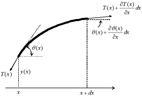
Figure 1: An infinitesimal string piece in tranverse motion.

A portion of a string in transverse motion is shown in Figure 1. The rest length of the element is $dx$. The variable internal tension is shown at cut locations, with a first order variation. For now, we shall assume constant density. Applying Newton’s Second Law to this piece, in both $x$ and $y$ directions, one gets the following equations of motion.

$$\left(T+dT\right)\cos(\theta+d\theta)-T\cos(\theta) = 0$$ (2)

$$\left(T+dT\right)\sin(\theta+d\theta)-T\sin(\theta) = a\ dm$$ (3)

where $dm$ is the total mass of the piece and $a$ is its acceleration of its center of mass (rotational effects are ignored). If a first order approximation is performed on

$$\cos(\theta+d\theta)=\cos(\theta)\cos(d\theta)-\sin(\theta)\sin(d\theta)$$ (4)

based on $\cos(d\theta)\approx 1$ and $\sin(d\theta)\approx d\theta$, one may argue that

$$\cos(\theta+d\theta)\approx\cos(\theta)-\sin(\theta)d\theta$$ (5)

which leads to

$$\cos\theta dT-T\sin\theta d\theta=0$$ (6)

$$\frac{dT}{T}=\tan\theta d\theta$$ (7)

in which second order differentials are neglected. Now, the last line can be easily integrated to give

$$T=C\left|\sec\theta\right|,\qquad(C>0)$$ (8)

which is the solution of the tension in terms of the slope angle. This is the part that is overlooked in previous studies. Without this form, a variable length assumption gives rise to non-linearity. It is this not-so-nice-looking result which actually restores the linearity of the final result.

Note that the absolute value operation automatically ensures the non-negativeness of the tension. However, after a closer examination, it can be shown to be unnecessary. When a section of $y(x,t)$ is obtained by left and right cuts, the angles of tangents at ends can also be viewed as the angle describing the angle of the tension vector. If one simply recalls that $y(x,t)$ is tacitly assumed to be a single valued function, the tension vector at left cut may only point towards the second and third quadrants, and the one at right end towards first and forth quadrants. Based on the way we defined the angles at each end, and the fact that $y$ is never allowed to be multi-valued, one concludes that $-\pi/2\leq\theta\leq\pi/2$, at any cut. Thus, $\cos\theta\geq 0$ and

$$T=C\sec\theta$$ (9)

Now, we concentrate on the second equation. Again, after expanding the trigonometric terms and applying first order approximations, one gets

$$\left(T+dT\right)\left(\cos d\theta\sin\theta+\sin d\theta\cos\theta\right)-T\sin(\theta) = a\ dm$$ (10)

$$\frac{dT}{d\theta}\sin\theta+T\cos\theta = a\frac{dm}{d\theta}$$ (11)

Using the solution for the tension:

$$C\tan^{2}\theta+C = a\frac{dm}{d\theta}$$ (12)

$$C\sec^{2}\theta = a\frac{dm}{d\theta}$$ (13)

is obtained. Next, we invoke the condition that all points of the string move in transverse direction. This simply implies that no mass is moving in or out of the region considered – a case of conservation of mass. Then,

$$dm=\rho A(x)ds=\rho A_{0}dx$$ (14)

where $\rho$ is the density, $A(x)$ is the cross-sectional area in current condition, $A_{0}$ is the uniform cross-sectional area at rest, and $ds=\sqrt{1+\left(\frac{\partial y}{\partial x}\right)^{2}}dx$ is the current length of the piece. Also, the acceleration $a$ can be approximated by $\frac{\partial^{2}y}{\partial t^{2}}$, since taking $\frac{\partial^{2}y}{\partial t^{2}}+\frac{\partial}{\partial x}\left(\frac{\partial^{2}y}{\partial t^{2}}\right)dx$, or any average of these, would lead to the same in the limit, assuming the smoothness of $\frac{\partial^{2}y}{\partial t^{2}}(x)$, of course. With these, the final equation becomes

$$\frac{d\theta}{dx}\sec^{2}\theta=\frac{\rho A_{0}}{C}\frac{\partial^{2}y}{\partial t^{2}}$$ (15)

Now, using the fact that $\frac{\partial y}{\partial x}=\tan\theta$, keeping time fixed, and using chain rule, one has

$$\frac{\partial^{2}y}{\partial x^{2}}=\frac{d}{dx}\left(\frac{dy}{dx}\right)=\frac{d}{d\theta}\left(\tan\theta\right)\frac{d\theta}{dx}=\frac{d\theta}{dx}\sec^{2}\theta$$ (16)

Therefore, the result becomes

$$\frac{\partial^{2}y}{\partial x^{2}} = \frac{\rho A_{0}}{C}\frac{\partial^{2}y}{\partial t^{2}}$$ (17)

$$y_{xx} = \frac{1}{c^{2}}y_{tt}$$ (18)

which is the well known classical linear wave equation, apart from the fact that nothing has been said about the nature of the constant $C$. This is the main result of this study.

3.1 An Alternative Method Leads To Much Stronger Result

The main result can actually be obtained in a nicer way: without arguing limits, infinitesimals, or first order approximations. We simply start with a really finite string piece. Let $T_{1}$ and $T_{2}$ be the tensions, and, $\theta_{1}$ and $\theta_{2}$ be the angles at left and right cuts, respectively. Then the force balance in $x$ direction dictates

$$T_{1}\cos\theta_{1}=T_{2}\cos\theta_{2}$$ (19)

This relation must hold for any segment (hence for any pair of end points $x_{i},x_{j}$), at all times. Letting $f(x,t)=T(x,t)\cos(\theta(x,t))$, the fact that $f(x_{i},t)=$ $f(x_{j},t)$ for all $x_{i},x_{j}$ leads to $f(x,t)=g(t)$, and in turn, the fact that $g(t_{i})=$ $g(t_{j})$ for all $t_{i},t_{j}\geq 0$ leads to the conclusion that $g(t)$ must be a constant. Hence, the result is

$$T\cos\theta=C$$ (20)

which, in a much more direct manner, gives the previous solution for the tension.

In obtaining this result we have not employed any differentials, infinitesimal elements, or approximations. Therefore, simply in order to be compatible with Newton’s Second Law, regardless of such details as whether bending is included or not, a constitutive model is utilized or not, and so on, and regardless of how complicated or higher order the model is, any string model must conform to this result, provided that only transverse motions are allowed. Of course, we are assuming that there are no shear forces at cut ends.

A similar approach can be applied for transverse motions. The force balance for the finite string piece in transverse direction gives

$$T_{2}\sin\theta_{2}-T_{1}\sin\theta_{1}=\int\limits_{x_{1}}^{x_{2}}y_{tt}dm$$ (21)

Now, we use the identity

$$\int\limits_{x_{1}}^{x_{2}}T\cos\theta d\theta=\left.T\sin\theta\right|_{x_{1}}^{x_{2}}-\int\limits_{x_{1}}^{x_{2}}\frac{dT}{d\theta}\sin\theta d\theta$$ (22)

which gives

$$T_{2}\sin\theta_{2}-T_{1}\sin\theta_{1}=\int\limits_{x_{1}}^{x_{2}}\left(T\cos\theta+\frac{dT}{d\theta}\sin\theta\right)d\theta$$ (23)

Here, we did not use partial derivatives since these relations must hold at any given time. Using the above identity one gets,

$$\int\limits_{x_{1}}^{x_{2}}y_{tt}dm=\int\limits_{x_{1}}^{x_{2}}\left(T\cos\theta+\frac{dT}{d\theta}\sin\theta\right)d\theta$$ (24)

Now, by applying $T\cos\theta=C$,

$$\int\limits_{x_{1}}^{x_{2}}y_{tt}dm=\int\limits_{x_{1}}^{x_{2}}\left(C+C\tan^{2}\theta\right)d\theta=\int\limits_{x_{1}}^{x_{2}}C\sec^{2}\theta d\theta$$ (25)

or

$$\int\limits_{x_{1}}^{x_{2}}\left(y_{tt}\frac{dm}{dx}-C\sec^{2}\theta\frac{d\theta}{dx}\right)dx=0$$ (26)

is obtained. Again using $\frac{\partial^{2}y}{\partial x^{2}}=\sec^{2}\theta\frac{d\theta}{dx}$ and $\frac{dm}{dx}=\rho A_{0},$one gets

$$\int\limits_{x_{1}}^{x_{2}}\left(\rho A_{0}y_{tt}-Cy_{xx}\right)dx=0$$ (27)

Since this must hold for all $x_{1},x_{2}$ we conclude that

$$\rho A_{0}y_{tt}-Cy_{xx} = 0$$ (28)

$$y_{xx} = \frac{\rho A_{0}}{C}y_{tt}$$ (29)

which is the same as the previous result.

As a conclusion, we state that there is no need for any smallness assumptions or first order approximations. Also notice that this equation is valid for both finite and infinite length strings.

4 On the Variability of Tension and Area

Assuming now that the solution to the wave equation is somehow obtained, one can get the solutions for the tension and cross-sectional area. The results are

$$T=C\sec\theta=C\sqrt{1+y_{x}^{2}}>0$$ (30)

and, from the conservation of mass equation,

$$A(x)=A_{0}\frac{dx}{ds}=A_{0}\cos\theta=\frac{A_{0}}{\sqrt{1+y_{x}^{2}}}>0$$ (31)

It is interesting to note that the product $T(x,t)A(x,t)=CA_{0}$ is conserved at all points and at all times. The tension and the cross-sectional area at a point are inversely proportional to each other. Another observation is that both depend on $y_{x}$ only.

Further, if $T$ is written as

$$T=C\frac{ds}{dx}$$ (32)

then, one may argue that if at some time, $t^{\ast}$, a string has $ds=dx$ everywhere, then the tension would be the same everywhere, say $T_{0}$, and one would necessarily have $T=C=T_{0}$. If such a configuration exists then the general solution would have to be given as

$$T=T_{0}\frac{ds}{dx}$$ (33)

Note that the existence of a configuration in which $ds=dx$ at $t^{\ast}$ everywhere, implies $y_{x}(x,t^{\ast})=0$ everywhere. Then, the inescapable conclusion is that $y(x,t^{\ast})$ is constant everywhere. Or, by a shift of coordinates, one can argue that $y(x,t^{\ast})=0$, everywhere. Here, we ignored the discussion of cases in which $ds=dx$ holds in finite intervals of distinct displacements.

It can now be stated that such configurations can always be contrived to exist: for example at those at times (say, $t<0$) at which the spring is unloaded and at rest. If the spring is considered to be unloaded and at rest prior to the application of initial conditions, then one may safely argue that $y(x,t)=y_{t}(x,t)=0,$for all $x$, and $t<0,$ (simply consider energy principles or the fact that this is a trivial solution of the string PDE, and thus realizable). This also forces that $y_{x}(x,t)=0$ in the same domain, giving $T(x,t)=T_{0}$ for all $x$, and $t<0$. As a result, $T_{0}$ is to be interpreted as the internal tension that would result had the spring been unloaded and at rest. Note that this is not equal to the tension in the initial condition.

4.1 What Happens at $t=0$?

Another counter intuitive conclusion pertains to the situation at initial condition. For any motion to ensue the string must be given an initial displacement or velocity, or both. Let’s consider a simple initial displacement as shown in Figure 2, with zero initial velocity.

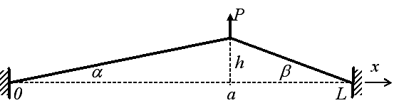
Figure 2: Initially displaced string under the action of a point force.

The force $P$ is what is needed to induce the shown displacement. Based on the results of this study, we can state that the tension at any point to the left of the external force is $T_{L}=T_{0}\sec\alpha=T_{0}\sqrt{1+\left(\frac{h}{a}\right)^{2}}$ and that to the right is $T_{R}=T_{0}\sec\beta=T_{0}\sqrt{1+\left(\frac{h}{L-a}\right)^{2}}$. Further, from the force balance in vertical direction at point $a$ one gets

$$P = T_{L}\sin\alpha+T_{R}\sin\beta$$ (34)

$$P = T_{0}\left(\tan\alpha+\tan\beta\right)$$ (35)

$$P = T_{0}h\left(\frac{1}{a}+\frac{1}{L-a}\right)=\frac{L}{a\left(L-a\right)}hT_{0}$$ (36)

Now, imagine a quasi-static application of the vertical force starting from zero, with zero deflection at point $a$, and gradually increasing to the value of $P$, at which time the deflection at $a$ becomes $h$. In such a process, one can simply integrate the work done by the vertical force in order to determine the net energy stored in the string at the initial condition. This gives

$$U_{0}=\frac{1}{2}\frac{Lh^{2}}{a\left(L-a\right)}T_{0}=\frac{1}{2}Ph$$ (37)

This is the internal energy stored that is converted into kinetic energy when the motion ensues. One may even define an equivalent spring stiffness at point $a$ as

$$k_{\text{eff-}a}=\frac{L}{\left(L-a\right)}\frac{T_{0}}{a}$$ (38)

Thus, in response to vertical forces, current string model responds like a linear spring, softest at the mid-point and stiffenning as $a$ aproaches to the boundaries. Also, the stiffness is linearly proportional to the initial tension. This behavior is quite familiar to those who have ever played a plucked string instrument such as a guitar. Such results are impossible to deduce from the classical treatments of ideal strings.

4.2 Does It Make Sense?

We immediately notice the situation of the string in regions where the slope vanishes. In such portions the tension is simply equal to the tension at rest. This could also be the case in initial condition. This is so even though the tension at neighboring points just ouside such portions can differ by a finite amount. For example, if there were two forces in the previous figure that were equal and applied at $a=L/3$ and $b=2L/3$ then, as the symmetry would require, the slope within middle section would have been zero and the tension therein would have been equal to $T_{0}$.

This behavior is due to the assumption that the string points are allowed to move only in transverse directions. The tension in the mid-section would stay constant because there would be no extension in that section. In reality, however, the tension in the mid-section would increase because some material would leave the region at both ends due to higher tensions in the first and third sections. Thus, in an analysis involving real material behavior the points must be allowed to move in all directions.

5 Energy Principles

Previously, we determined the internal energy corresponding to an initial displacement caused by a point force. In this section we present a generalization that enables one to formulate the string problem using energy methods. In addition, the results help validate the main results of this study.

The internal energy is stored via changes in tension and length (area). Since both of these depend only on spatial derivative of the displacement, the energy stored while in motion will be the same as that in a static case, as long as the displacement fields are identical. Therefore, given $u(x)=y(x,t=t^{\ast})$, where $t^{\ast}$ is a particular instant, one can argue that the internal energy at this instant will be the same as the one under the action of a suitable force distribution which, in static equilibrium, induces the displacement field $u(x)$.

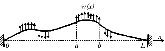
Figure 3: String displacement under the action of a piece-wise continuous force distribution.

We now restrict the consideration to piece-wice smooth force distributions. An example of this is shown in Figure 3. For instance, $w(x)$ is the external force distribution defined on the open interval $(a,b)$. Now, imagine a small piece cut inside this domain, with internal tensions appearing at cut ends, defined as before (see, Figure 4). A vertical force balance requires

$$(T+dT)\sin\left(\theta+d\theta\right)-T\sin\theta=-\bar{w}(x)dx$$ (39)

where $\bar{w}(x)$ is a representative value, an average or that obtained by applying the mean value theorem. Using $T=T_{0}\sec\theta$, this gives

$$\bar{w}(x) = -T_{0}\frac{\left(\tan\left(\theta+d\theta\right)-\tan\theta\right)}{dx}$$ (40)

$$= -T_{0}\frac{\left(\tan\left(\theta+d\theta\right)-\tan\theta\right)}{d\theta}\frac{d\theta}{dx}$$ (41)

In the limit $\lim_{dx\rightarrow 0}\bar{w}(x)$ one obtains

$$w(x)=-T_{0}\sec^{2}\theta\frac{d\theta}{dx}$$ (42)

But, from Equation 16, this simply is

$$w(x)=-T_{0}u_{xx}$$ (43)

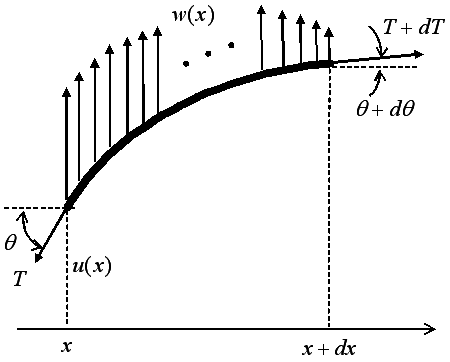
Figure 4: A differential string element in transverse motion due to a continuous force distribution.

That is, the force distribution necessary to induce a static deflection of $u(x)$ is proportional to $u_{xx}$. This also indicates that the smoothness of $u$ is required up to the second derivative – only in a piecewise manner.

Now, let $U$ be the internal energy of the string in configuration $u(x)$, and $U_{0}$ be that in unloaded configuration at rest ($u(x)=0$, everywhere). Then, by the first law of thermodynamics, we must require

$$U-U_{0}=W(w)$$ (44)

where $W(w)$ is the work done by the external forces in bringing the string from the initial to the final configuration.

Next, we aim at calculating this work done. For this, imagine that the string is brought to the final configuration via a quasi-static process in which all intermediate configurations are given by

$$h(x)=\alpha u(x)\qquad\alpha\in[0,1]$$ (45)

The corresponding force distributions would be given by: $w(x)=-\alpha T_{0}u_{xx}$. The work done in going from $h$ to $h+dh$, due to a variation $d\alpha$, is given by

$$dW=\left[w(x)dx\right]dh=\left[-\alpha T_{0}u_{xx}dx\right](ud\alpha)$$ (46)

Thus, the net work done can be found from the integral

$$W=\int_{a}^{b}\int_{0}^{1}\left(-T_{0}uu_{xx}\right)\alpha d\alpha dx=-\frac{1}{2}T_{0}\int_{a}^{b}uu_{xx}dx$$ (47)

where $a,b$ are the values of $x$ at boundaries, and either one can be taken at infinity. The final integral can be simplified using integration by parts as

$$W=-\frac{1}{2}T_{0}\left[\left.uu_{x}\right|_{a}^{b}-\int_{a}^{b}u_{x}^{2}dx\right]$$ (48)

If one measures the internal energy by using $U_{0}$ as the reference, that is $U-U_{0}\rightarrow U$, then the conclusion is

$$U=\frac{1}{2}T_{0}\int_{a}^{b}u_{x}^{2}dx-\frac{1}{2}T_{0}\left(\left.uu_{x}\right|_{a}^{b}\right)$$ (49)

This is the internal energy stored due to the work done by external forces. When in motion, the same displacement field would represent the same internal energy.

Now, we concentrate on the case of fixed boundaries (we mean, $u(a)=u(b)=0$) for which the second term vanishes. For other cases refer to [6], where it is shown that the same equation of motion is obtained, only with certain restrictions at boundaries. Hence, for fixed boundaries, we get

$$U(t)=\frac{1}{2}T_{0}\int_{a}^{b}y_{x}^{2}dx$$

Quite surprisingly, this is exactly the same as the one obtained in classical treatments with constant tension assumption. For example, in [1] the internal energy is calculated using the assumption that the string undergoes an extension under a constant tension, $\tau_{0}$, which yields $U=\tau_{0}\int\left(\sqrt{1+y_{x}^{2}}-1\right)dx$. After expanding the radical in series and ignoring the terms higher than the linear, they get $U=\frac{1}{2}\tau_{0}\int y_{x}^{2}dx$. This is done even after inextensibility is assumed! The question that remains is that whether or not this is merely a lucky coincidence, despite so many conflicting model assumptions in classical string models.

If, now, one writes $K(t)=\frac{1}{2}\int_{a}^{b}\rho^{\ast}y_{t}^{2}dx$ for the kinetic energy, where $\rho^{\ast}$ is the linear density, then the Lagrangian of the system is

$$\pounds(t)=K(t)-U(t)=\frac{1}{2}\int_{a}^{b}\left[\rho^{\ast}y_{t}^{2}-T_{0}y_{x}^{2}\right]dx$$ (50)

which is the same as in [1]. Therefore, the same equation of motion is obtained upon application of Hamilton’s principle and variational methods (see also [2], [6]). This proves that the main results of this study are also consistent with energy approaches.

6 Variability of Area and Density at Rest

Let us assume that for some reason the unloaded string has a spatially varying cross-sectional area $A_{0}$ and density $\rho_{0}$. The development presented using the alternative method is still valid up to Equation 26. Hence, we have

$$\int\limits_{x_{1}}^{x_{2}}\left(y_{tt}\frac{dm}{dx}-Cy_{xx}\right)dx=0$$ (51)

Also, due to pure transverse motion assumption, the mass is conserved inside any finite piece. Hence

$$\int\limits_{x_{1}}^{x_{2}}dm=\int\limits_{x_{1}}^{x_{2}}\rho(x,t)A(x,t)ds=\int\limits_{x_{1}}^{x_{2}}\rho_{0}(x)A_{0}(x)dx$$ (52)

or, arguing as before,

$$\frac{dm}{dx}=\rho_{0}(x)A_{0}(x)$$ (53)

Thus,

$$\int\limits_{x_{1}}^{x_{2}}\left(y_{tt}\rho_{0}(x)A_{0}(x)-T_{0}y_{xx}\right)dx=0$$ (54)

and, one obtains

$$y_{xx}=\frac{\rho_{0}(x)A_{0}(x)}{T_{0}}y_{tt}=\frac{\rho_{0}^{\ast}(x)}{T_{0}}y_{tt}$$ (55)

where $\rho_{0}^{\ast}$ is the linear density distribution at rest. This is the most general equation of motion for transverse vibrations of a string. Note again that in obtaining this result neither finiteness of length nor any boundary conditions are argued. A similar result is obtained in [6], although all other unnecessary assumption are still used.

7 Conclusion

A new approach to the transverse motion of ideal strings is presented, in which most of the approximations and assumptions of classical models are removed. The new model allows variable tension and length, and, arbitrarily large displacements and derivatives. Despite these relaxations the resulting equation of motion is shown to be exactly the same as that of the classical linear model. The result is obtained in three distinct ways: using differential elements, finite elements, and energy principles. Another new result relating force distributions to the second spatial derivative of displacement is also presented. Finally, an equation of motion for variable cross-sectional area and density is presented.

It must be cautioned here that, although the resulting equation of motion is the same as that in previous studies, with the analyses presented in this study we now have a variable tension and large deflection model.

References

- [1] Sagan, H., Boundary and Eigenvalue Problems in Mathematical Physics, 1989, Dover Pub. (Original publication, 1961, Wiley)
- [2] Byron, F. W. and Fuller, R. W., Mathematics of Classical and Quantum Physics, 1992, Dover Pub. (Original publications, 1969, 1970: General Publishing Co., Canada; and Constable and Company, UK)
- [3] Gottlieb, H. P. W., 1990, ”Non-linear Vibration of a Constant-Tension String”, Journal of Sound and Vibration, v. 143, pp 455 – 460.
- [4] Lai, S. K., Xiang, Y., et al., 2008, ”Higher-Order Approximate Solutions For Nonlinear Vibration of a Constant-Tension String”, Journal of Sound and Vibration, v. 317, pp 440 – 448.
- [5] Rao, G. V., 2002, ”Moderately Large Amplitude Vibrations of a Constant Tension String: a Numerical Experiment”, Journal of Sound and Vibration, v. 263, pp 227 – 232.
- [6] Weinstock, R., Calculus of Variations, 1974, Dover Pub. (Original publications, 1952: General Publishing Co., Canada; and, Constable and Company, UK)
- [7] Benson, D. J., Music: A Mathematical Offering, 2007, Cambridge University Press, UK and USA.