Utility Fair Optimisation of Antenna Tilt Angles in LTE Networks

Abstract

We formulate adaptation of antenna tilt angle as a utility fair optimisation task. This optimisation problem is non-convex, but in this paper we show that under reasonable conditions it can be reformulated as a convex optimisation. Using this insight, we develop a lightweight method for finding the optimal antenna tilt angles, making use of measurements which are already available at base stations, and suited to distributed implementation.

I Introduction

The antenna tilt angle of wireless base-stations is known to be a key factor in determining cell coverage and to play a significant role in interference management [1], [2]. While traditionally adjustment of tilt angle has largely been carried out manually, modern base stations increasingly allow automated adjustment. This creates the potential for more dynamic adaptation of tilt angle, for example to better match cell coverage to the distribution of user equipments and traffic, to reduce coverage holes created by failures in neighbouring stations, to better manage interference from the user deployment of femtocells, etc. The benefits of self configuration and self optimisation are already recognised in LTE release 9 [3], and automated adaptation of tilt angle in particular has been the subject of recent interest.

In this paper we formulate adaptation of antenna tilt angle as a utility fair optimisation task. Namely, the objective is to jointly adjust antenna tilt angles within the cellular network so as to maximise user utility, subject to network constraints. Adjustments at base stations must be carried out jointly in a co-ordinated manner in order to manage interference. This optimisation problem is non-convex, but in this paper we show that under certain conditions it can be reformulated as a convex optimisation. Specifically, we show that (i) in the high signal to interference ratio (SINR) operating regime and with an appropriate choice of decision variables, the optimisation is convex for any concave utility function, and (ii) in any SINR regime the optimisation can be formulated in a convex manner when the objective is a proportional fair rate allocation. Since the optimisation is not well-suited to solution using standard dual methods, we develop a primal-dual method for finding the optimal antenna tilt angles. This approach is lightweight, making use of measurements which are already available at base stations, and suited to distributed implementation.

The rest of the paper is organized as follows. In Section II we summarize the existing work in the area. In Section III we introduce our network model, which is based on 3GPP standard , and in Section IV we analyse its convexity properties in the high SINR regime. In Section V we extend the analysis to general SINR regimes. In Section VI we carry out a performance evaluation of a realistic setup and finally, in Section VIII, we summarise our conclusions.

II Related Work

The analysis and modelling of the impact of the antenna tilt angle on cell performance has been well studied, see for example [4, 5] and references therein. Recently, self-optimisation of tilt angle has started to attract attention, but most of this work makes use of heuristic approaches. In [6] a heuristic method is proposed for adjusting tilt to maximise average spectral efficiency within the network, while [7] proposes a combination of fuzzy and reinforcement learning. In [8] simulated annealing is considered for joint self-configuration of antenna tilt angle and power and in [9] a non-cooperative game approach between neighbouring base stations is studied. Offline planning of tilt angle is considered, for example, in [10], using a heuristic search method combined with a mixed integer local search. In the present paper, we take a more formal, rigorous approach and show that tilt angle optimisation can, in fact, be formulated as a convex problem. Building on this result, we then introduce a lightweight distributed algorithm based on primal-dual subgradient updates and show that this algorithm is guaranteed to converge arbitrarily closely to the network optimum.

III Network Model

III-A Network Architecture

The network consists of a set ${\mathcal{B}}$ of base stations and a set ${\mathcal{U}}$ of User Equipment (UE), with UE $u\in{\mathcal{U}}$ receiving downlink traffic transmitted from base station $b(u)\in{\mathcal{B}}$. For base stations with sectoral antennas, we define a separate element in ${\mathcal{B}}$ for each antenna. We denote the $(x,y)$ geographical co-ordinates of base station $b$ by $(x_{b},y_{b})$ and of user equipment $u$ by $(x_{u},y_{u})$. The distance between user $u$ and base station $b$ is therefore given by

$$d_{b,u}=\sqrt{(x_{u}-x_{b})^{2}+(y_{u}-y_{b})^{2}}$$ (1)

III-B Antenna Gain and Path Loss

The received power on sub-carrier $n$ from base station $b\in{\mathcal{B}}$ at user $u\in{\mathcal{U}}$ is given by $\tilde{G}_{b,u}(\theta_{b})\rho_{b,u}P_{b,n}$, where $\tilde{G}_{b,u}(\theta_{b})$ is the base station antenna gain, $\rho_{b,u}$ the path loss between $b$ and $u$, $P_{b,n}$ is the base station transmit power for sub-carrier $n$ . For simplicity, shadowing and fast fading are not considered in the equations. We model path loss, as recommended in [11], by

$$\rho_{b,u}=\rho_{0}d_{b,u}^{-\beta}$$ (2)

with fixed path loss factor $\rho_{0}$, path loss exponent $\beta$ and distance $d$ in kilometres. For a given antenna type, the antenna gain $~{}\tilde{G}_{b,u}(\theta_{b})$ can be determined given the relative positions of $b$ and $u$, the antenna tilt angle $\theta_{b}$ and the azimuth angle $\phi_{b}$. With regard to the latter, changing the tilt and/or azimuth angles changes the direction of the antenna’s main lobe, see Fig 1. We will assume that the azimuth angle is held fixed but allow the antenna tilt angle to be adjusted within the interval $[\underline{\theta},\bar{\theta}]$. Following [11], the antenna gain can then be modelled by:

$$\tilde{G}_{b,u}(\theta_{b})=\tilde{G}_{0}\tilde{G}_{v}(\theta_{b},d_{b,u})$$ (3)

where $\tilde{G}_{0}$ is the maximum gain of the antenna,

$$\tilde{G}_{v}(\theta_{b},d_{b,u}) =10^{-1.2\left(\frac{\theta_{b,u}-\theta_{b}}{\theta_{3dB}}\right)^{2}}$$ (4)

is the antenna vertical attenuation, $\theta_{b,u}=\tan^{-1}\left(h/d_{b,u}\right)$, $h$ is the height difference between the base station and UE (which, for simplicity, we assume is the same for all base stations and users) and $\theta_{3dB}$ the vertical half power beam width of the antenna. Figure 2 illustrates the ability of (4) to accurately model the main lobe of an antenna which is popular in cellular networks.

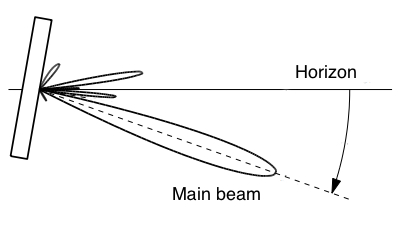
Figure 1: Schematic illustrating relationship between antenna main lobe and tilt angle.

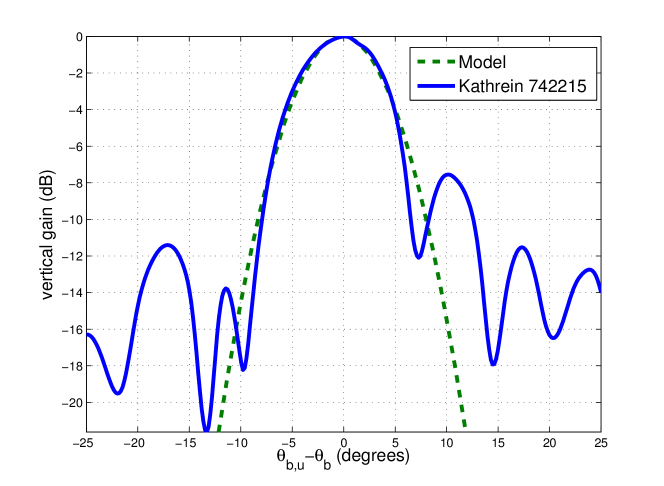
Figure 2: Comparison of antenna main lobe vertical gain model (4) (dashed line) and measured antenna gain (solid line) for a Kathrein 742215 antenna, $\theta_{3dB}=9^{\circ}$.

It will prove useful to use the quantity $G_{v}(\theta_{b},d_{b,u}):=\log{\tilde{G}_{v}(\theta_{b},d_{b,u})}$. It will also prove useful to consider the following linear approximation $\hat{G}_{v}(\theta_{b},d_{b,u})$ to antenna gain exponent $G_{v}(\theta_{b},d_{b,u})$ about tilt angle $\theta_{0}$,

$$\hat{G}_{v}(\theta_{b},d_{b,u})=\frac{-1.2\log 10}{\theta_{3dB}^{2}}\Big{(}(\theta_{b,u}-\theta_{0})^{2}+2(\theta_{b,u}-\theta_{0})\theta_{b}\Big{)}$$ (5)

This linear approximation is illustrated by the solid line in Figure 3. It is reasonably accurate provided adaptation of the antenna angle $\theta_{b}$ does not cause $\theta_{b,u}-\theta_{b}$ to change sign (in which case the side of the main antenna lobe facing the user changes and so the slope of the linear approximation changes sign). This is assumed to be the case for the antennas of base stations other than that to which the UE is associated, which is only a mild assumption since otherwise interference from these base stations can be expected to be excessive.

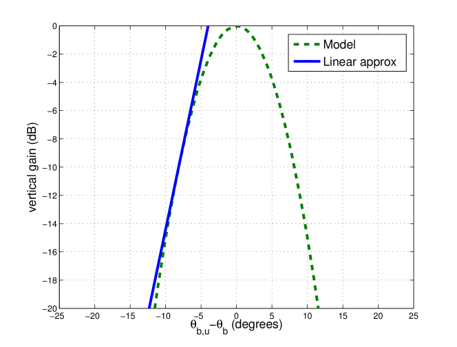
Figure 3: Illustrating linear approximation $\hat{G}_{v}(\theta_{b},d_{b,u})$ to $G_{v}(\theta_{b},d_{b,u})$, $\theta_{3dB}=9^{\circ}$.

III-C User Throughput

The downlink throughput of the user equipment $u\in{\mathcal{U}}$ associated with base station $b(u)$ is given by:

$$R_{u}(\Theta)=\min\{\bar{r},r_{u}(\Theta)\},\quad u\in{\mathcal{U}}$$ (6)

where $\Theta$ is the vector $[\theta_{b}]$, $b\in{\mathcal{B}}$ of tilt angles, $\bar{r}$ is the maximum achievable throughput (limited by the available modulation and coding schemes), and

$$r_{u}(\Theta)=\frac{w}{N_{sc}}\sum_{n=1}^{N_{sc}}\log(1+\kappa\gamma_{u,n}(\Theta))$$ (7)

Here $N_{sc}$ is the number of sub-carriers, $w$ the channel bandwidth, $\kappa$ a loss factor capturing non-ideal coding etc, and $\gamma_{u,n}(\Theta)$ SINR on sub carrier $n$ for user $u$,

$$\gamma_{u,n}(\Theta)=\frac{H_{u}(\theta_{b(u)})}{\sum_{c\in{\mathcal{B}}\setminus\{b(u)\}}\hat{H}_{u}(c)+\eta_{u,n}}$$ (8)

where $H_{u}(\theta_{b}):=e^{G_{b,u}(\theta_{b})}\rho_{b,u}P_{b,u}$ is the received power from base station $b(u)$ by user $u$, $\hat{H}_{u}(\theta_{c}):=e^{\hat{G}_{c,u}(\theta_{c})}\rho_{c,u}P_{c,u}$ is the received power from base station $c\neq b(u)$ by user $u$ and $\eta_{u,n}$ the channel noise for user $u$ on sub carrier $n$. Observe that in $\hat{H}_{u}(\theta_{c})$ we make use of linear approximation $\hat{G}_{v}$.

IV High SINR Regime

In the high SINR regime, the downlink throughput (6) can be accurately approximated by

$$\hat{R}_{u}(\Theta)=\min\{\bar{r},\hat{r}_{u}(\Theta)\},\quad u\in{\mathcal{U}}.$$ (9)

where

$$\hat{r}_{u}(\Theta)=\frac{w}{N_{sc}}\sum_{n=1}^{N_{sc}}\log(\kappa\gamma_{u,n}(\Theta))$$ (10)

IV-A Utility Fair Optimisation of Tilt Angle

Under the assumption of high SINR operation, we can formulate the selection of antenna tilt angles as the following optimisation problem $(P1)$:

$$\max_{\Theta} \sum_{u\in{\mathcal{U}}}U(\hat{R}_{u}(\Theta))$$ (11)

$$s.t.\quad \underline{\theta}\leq\theta_{b}\leq\bar{\theta},\quad b\in{\mathcal{B}}$$ (12)

$$\underline{r}\leq\hat{R}_{u}(\Theta),\quad u\in{\mathcal{U}}$$ (13)

where $U(\cdot)$ is a concave increasing utility function and $\underline{r}\geq 0$. Constraint (12) captures restrictions on the range of feasible antenna tilt angles, while (13) ensures that each user receives a specified minimum throughput (which is expected to mainly be important for users at the edge of a cell who might otherwise be assigned too low a throughput).

IV-B Convexity Properties

Lemma 1

$\log H_{u}(\theta_{b})$ is strictly concave in $\theta_{b}$.

Proof:

We have

$$\log H_{u}(\theta_{b}) =G_{b,u}(\theta_{b})+\log\rho_{b,u}+\log P_{b,u}$$

$$=-1.2\frac{\log 10}{\theta_{3dB}^{2}}\left(\theta_{b,u}-\theta_{b}\right)^{2}+\log\rho_{b,u}+\log P_{b,u}$$

Now $\log\rho_{b,u}$, $\log P_{b,u}$, $\theta_{3dB}$ and $\theta_{b,u}$ are constants, so we only need to consider concavity with respect to $\theta_{b}$. It can be verified that $\frac{d^{2}\log H_{u}(\theta_{b})}{d\theta_{b}^{2}}=-2.4\frac{\log 10}{\theta_{3dB}^{2}}<0$. ∎

Lemma 2

$\log\left(\sum_{c\in{\mathcal{B}}\setminus\{b(u)\}}\hat{H}_{u}(\theta_{c})+\eta_{u,n}\right)$ is convex.

Proof:

Rewrite as
$\log\left(\sum_{c\in{\mathcal{B}}\setminus\{b(u)\}}e^{\hat{G}_{c,u}(\theta_{c})+\log\rho_{c,u}P_{c,u}}+\eta_{u,n}\right)$. This can be expressed as $\log\left(\sum_{c\in{\mathcal{B}}\setminus\{b(u)\}}e^{h_{c,u}(\theta_{c})}+\eta_{u,n}\right)$ with $h_{c,u}(\theta_{c}):=\hat{G}_{c,u}(\theta_{c})+\log\rho_{c,u}P_{c,u}$. By [12, p74], the log of a sum of exponentials is convex. The additive term $\eta_{u,n}$ acts as a translation and by  [12, p79] convexity is preserved under translation. By approximation (5), the function $h_{c,u}(\theta_{c})$ is affine in $\theta_{c}$, and by [12, p79] when composed with the log of a sum of exponentials the resulting function remains convex. ∎

It follows from Lemmas 1 and 2 that

Theorem 1

$\hat{R}_{u}(\Theta)$ is concave in $\Theta$.

Proof:

Recalling from (8) and (10):

$$\hat{r}_{u}(\Theta)=\frac{w}{N_{sc}}\sum_{n=1}^{N_{sc}} \bigg{(} \log\kappa+\log H_{u}(\theta_{b(u)})$$ (14)

$$\>-\log\big{(}\sum_{c\in{\mathcal{B}}\setminus\{b(u)\}}\hat{H}_{u}(c)+\eta_{u,n}\big{)}\bigg{)}$$

By Lemmas 1 and 2, $\hat{r}_{u}(\Theta)$ is concave in $\Theta$. Since the $\min$ function is concave and nondecreasing, it follows that $\hat{R}_{u}(\Theta):=\min\{\hat{r}_{u}(\Theta),\bar{r}\}$ is also concave in $\Theta$. ∎

Note that $\hat{R}_{u}(\Theta)$ is not strictly concave in $\Theta$ since $\log H_{u}(\theta_{b(u)})$ is only strictly concave in $\theta_{b}(u)$ but not in the other elements of $\Theta$. Nevertheless, under mild conditions $\sum_{u\in{\mathcal{U}}}\hat{R}_{u}(\Theta)$ is strictly concave in $\Theta$:

Theorem 2

Suppose ${\mathcal{B}}=\cup_{u\in{\mathcal{U}}}b(u)$, i.e. every base station $b\in{\mathcal{B}}$ has at least one associated UE $u\in{\mathcal{U}}$. Then $\sum_{u\in{\mathcal{U}}}\hat{r}_{u}(\Theta)$ is strictly concave in $\Theta$ (and so the solution to problem $(P1)$ is unique).

Proof:

We have

$$\sum_{u\in{\mathcal{U}}}\hat{r}_{u}(\Theta)=\frac{w}{N_{sc}}\sum_{n=1}^{N_{sc}} \bigg{(} \sum_{u\in{\mathcal{U}}}\log\kappa+\sum_{u\in{\mathcal{U}}}\log H_{u}(\theta_{b(u)})$$

$$\>-\sum_{u\in{\mathcal{U}}}\log(\sum_{c\in{\mathcal{B}}\setminus\{b(u)\}}\hat{H}_{u}(c)+\eta_{u,n})\bigg{)}$$

Recall $H_{u}(\theta_{b(u)})$ is strictly concave in $\theta_{b(u)}$ (by Lemma 1). The sum $\sum_{u\in{\mathcal{U}}}\log H_{u}(\theta_{b(u)})$ is therefore strictly concave in every $\theta_{b}$, $b\in\cup_{u\in{\mathcal{U}}}b(u)={\mathcal{B}}$. It is therefore strictly concave in $\Theta$ (in more detail, for any $\Theta^{1}$, $\Theta^{2}$ and $\alpha\in[0,1]$ we have $\sum_{u\in{\mathcal{U}}}\log H_{u}(\alpha\theta^{1}_{b(u)}+(1-\alpha)\theta^{2}_{b(u)})>\sum_{u\in{\mathcal{U}}}\left(\alpha\log H_{u}(\theta^{1}_{b(u)})+(1-\alpha)\log H_{u}(\theta^{2}_{b(u)})\right)=\alpha\sum_{u\in{\mathcal{U}}}\log H_{u}(\theta^{1}_{b(u)})+(1-\alpha)\sum_{u\in{\mathcal{U}}}\log H_{u}(\theta^{2}_{b(u)})$). The result then follows from the fact that the sum of a strictly concave function and a concave function is strictly concave. ∎

And we have the following corollary,

Corollary 1

When each base station has at least one user with throughput less that $\bar{r}$, then $\sum_{u\in{\mathcal{U}}}\hat{R}_{u}(\Theta)$ is strictly concave in $\Theta$.

Proof:

Let $\bar{{\mathcal{U}}}\subset{\mathcal{U}}$ denote the set of users with throughput less than $\bar{r}$. When each base station has at least one user with throughput less that $\bar{r}$ then ${\mathcal{B}}=\cup_{u\in\bar{{\mathcal{U}}}}b(u)$. Now $\sum_{u\in\bar{{\mathcal{U}}}}\hat{R}_{u}(\Theta)=\sum_{u\in\bar{{\mathcal{U}}}}\hat{r}_{u}(\Theta)$ is strictly concave in $\Theta$ by Theorem 2. It then follows immediately that $\sum_{u\in{\mathcal{U}}}\hat{R}_{u}(\Theta)=\sum_{u\in\bar{{\mathcal{U}}}}\hat{R}_{u}(\Theta)+\sum_{u\in U\setminus\bar{{\mathcal{U}}}}\bar{r}$ is strictly concave in $\Theta$. ∎

IV-C Convex Optimisation

The objective function in optimisation problem (P1) is concave in $\Theta$ (since $U(\cdot)$ is concave increasing and $\hat{R}_{u}(\Theta)$ is concave by Theorem 1, then $U(\hat{R}_{u}(\Theta))$ is concave) and constraints (12)-(13) are linear (and so convex). Hence, optimisation problem (P1) is convex. It follows immediately that a solution exists. The Slater condition is satisfied and so strong duality holds.

IV-D Difficulty of Using Conventional Dual Algorithms

The Lagrangian is

$$L(\Theta,\Lambda) =-\sum_{u\in{\mathcal{U}}}U(\hat{R}_{u}(\Theta))+\sum_{u\in{\mathcal{U}}}\lambda_{u}^{1}(\underline{r}-\hat{R}_{u}(\Theta))$$ (15)

$$+\sum_{b\in{\mathcal{B}}}\lambda^{2}_{b}(\underline{\theta}-\theta_{b})+\sum_{b\in{\mathcal{B}}}\lambda^{3}_{b}(\theta_{b}-\bar{\theta})$$

where $\Lambda$ denotes the set of multiplers $\lambda_{u}^{1}$, $\lambda_{b}^{2}$, $\lambda_{b}^{3}$, $u\in{\mathcal{U}}$, $b\in{\mathcal{B}}$. The dual function is $g(\Lambda):=L(\Theta^{*}(\Lambda),\Lambda)$, where $\Theta^{*}(\Lambda)=\arg\max_{\Theta}L(\Theta,\Lambda)$. The main KKT conditions are $dL(\Theta,\Lambda)/d\theta_{b}=0$, $b\in{\mathcal{B}}$. That is,

$$\sum_{u\in{\mathcal{U}}}\left(1+\lambda_{u}^{1}\right)\partial_{\theta_{b}}U(\hat{R}_{u}(\Theta))=\lambda_{b}^{3}-\lambda_{b}^{2},\quad b\in{\mathcal{B}}$$ (16)

Given $\Lambda$, we can use (16) to find $\Theta^{*}(\Lambda)$. The optimal vector of multipliers is $\Lambda^{*}=\arg\max_{\Lambda\geq 0}g(\Lambda)$. Since $g(\Lambda)$ is concave, a standard dual function approach is to find $\Lambda^{*}$ using subgradient ascent techniques, and then find the optimal tilt angle $\Theta^{*}(\Lambda^{*})$. However, solving (16) to obtain the primal variables is tricky in general since it imposes complex, implicit dual constraints for a solution to exist. Consequently, the dual subgradient approach is unattractive for solving problem (P1).

IV-E Distributed Algorithm for Finding Optimal Solution

We consider the following primal-dual algorithm:

Initialise: $t=0$, $\Theta(0)$, $\Lambda(0)$, step size $\alpha>0$
do
$\displaystyle\theta_{b}(t+1)$ $\displaystyle=\theta_{b}(t)-\alpha\partial_{\theta_{b}}L(\Theta(t),\Lambda(t)),\quad\quad\ \theta_{b}\in{\mathcal{B}}$ (17) $\displaystyle\lambda_{u}^{1}(t+1)$ $\displaystyle=\left[\lambda_{u}^{1}(t)+\alpha\partial_{\lambda_{u}^{1}}L(\Theta(t),\Lambda(t))\right]^{+},\ u\in{\mathcal{U}}$ (18) $\displaystyle\lambda_{b}^{i}(t+1)$ $\displaystyle=\left[\lambda_{b}^{i}(t)+\alpha\partial_{\lambda_{b}^{i}}L(\Theta(t),\Lambda(t))\right]^{+},\ b\in{\mathcal{B}},i=2,3$ (19) $\displaystyle t\leftarrow t+1$ loop

Algorithm 1 High SINR

where in Algorithm 1 projection $[z]^{+}$ equals $z$ when $z\geq 0$ and $0$ otherwise,

$$\partial_{\theta_{b}}L(\Theta,\Lambda) =-\sum_{u\in{\mathcal{U}}}\left(1+\lambda_{u}^{1}\right)\partial_{\theta_{b}}U(\hat{R}_{u}(\Theta))-\lambda^{2}_{b}+\lambda^{3}_{b}$$ (20)

$$\partial_{\lambda_{u}^{1}}L(\Theta,\Lambda) =\underline{r}-\hat{R}_{u}(\Theta)$$ (21)

$$\partial_{\lambda_{b}^{2}}L(\Theta,\Lambda) =\underline{\theta}-\theta_{b}$$ (22)

$$\partial_{\lambda_{b}^{3}}L(\Theta,\Lambda) =\theta_{b}-\bar{\theta}$$ (23)

and $\partial_{\theta_{b}}U(\hat{R}_{u}(\Theta))$ denotes any subgradient of $U(\hat{R}_{u}(\Theta))$ with respect to $\theta_{b}$.

Observe that each iteration (17)-(19) of Algorithm 1 simultaneously updates both the primal variable $\Theta$ and the multipliers $\lambda_{u}^{1}$, $\lambda_{b}^{2}$, $\lambda_{b}^{3}$. It possesses the following convergence property:

Lemma 3

For Algorithm 1 suppose $(\Theta(t),\Lambda(t))$ is bounded for all $t$. Then there exists constant $M\geq 0$ such that

$$0 \leq \frac{1}{t}\sum_{\tau=0}^{t}\Big{(}L(\Theta(\tau),\Lambda^{*})-L(\Theta^{*},\Lambda(\tau))\Big{)}\leq\frac{\Delta}{2\alpha t}+\frac{\alpha M}{2}$$

where $(\Theta^{*},\Lambda^{*})$ is a solution to optimisation problem (P1), $\Delta=||\Theta(0)-\Theta^{*})||_{2}^{2}+||\Lambda(0)-\Lambda^{*}||_{2}^{2}$ and $||\cdot||_{2}$ denotes the usual Euclidean norm.

Proof:

Optimisation problem $(P1)$ is convex, the objective and constraint functions are differentiable and the Slater condition is satisfied. The result now follows by direct application of Lemma 8 in the Appendix. ∎

Since $\Delta/(2\alpha t)\rightarrow 0$ as $t\rightarrow\infty$, Lemma 3 tells us that update (17)-(19) converges to a ball around an optimum $(\Theta^{*},\Lambda^{*})$, the size of the ball decreasing with step size $\alpha$. The size of the ball is measured in terms of metric $L(\Theta,\Lambda^{*})-L(\Theta^{*},\Lambda)$, and recall that by complementary slackness $L(\Theta^{*},\Lambda^{*})=\sum_{u\in{\mathcal{U}}}U(\hat{R}_{u}(\Theta^{*}))$.

IV-F Message Passing and Implementation

Algorithm 1 can be implemented in a distributed manner. Namely, each base station $b\in{\mathcal{B}}$ carries out local tilt angle updates according to (17) and (19), and also carries out update (18) for each user $u$ associated with base station $b$. For this, each base station $b$ needs to evaluate (20)-(23). Evidently (21)-(23) can be evaluated using locally available information (the tilt angle of base station $b$ and the current downlink throughput of user $u$ associated with base station $b$). In contrast, evaluating (20) requires information sharing between base stations. Specifically, it is necessary to evaluate

$$\sum_{u\in{\mathcal{U}}}\frac{\partial\hat{r}_{u}}{\partial\theta_{b}} =\sum_{u\in\{u\in{\mathcal{U}}:b(u)=b\}}\frac{\partial\hat{r}_{u}}{\partial\theta_{b}}+\sum_{u\in\{u\in{\mathcal{U}}:b(u)\neq b\}}\frac{\partial\hat{r}_{u}}{\partial\theta_{b}}$$ (24)

The first term in (24) is the sensitivity of the throughput of users associated to base station $b$ to changes in its tilt angle $\theta_{b}$. This can either be directly measured by base station $b$ (by perturbing the tilt angle), or calculated using

$$\frac{\partial\hat{r}_{u}}{\partial\theta_{b}} =\frac{w}{N_{sc}}\sum_{n=1}^{N_{sc}}\frac{\partial G_{v}(\theta_{b},d_{b,u})}{\partial\theta_{b}}$$ (25)

where

$$\frac{\partial G_{v}(\theta_{b},d_{b,u})}{\partial\theta_{b}}=\frac{2.4\log 10}{\theta_{3dB^{2}}}(\theta_{b(u),u}-\theta_{b})$$ (26)

This calculation requires knowledge of the pointing angle $\theta_{b(u),u}$ between base station $b$ and user $u$. This pointing angle can be determined from knowledge of the location of users, information which is usually available to modern base stations since Location Based Services (LBS) are of high importance for mobile network providers. For example, in the US carriers are required by FCC to provide location-based information of the mobile users for E911 services and to within a specified accuracy [13]. Within Release 9 of 3GPP a set of enhanced positioning methods are standardized for LTE[14].

The second term in (24) is the sensitivity of the throughput of users associated to base stations other than $b$ to changes in tilt angle $\theta_{b}$. This can be calculated as

$$-\frac{1}{N_{sc}}\sum_{u\in\{u\in{\mathcal{U}}:b(u)\neq b\}}\sum_{n=1}^{N_{sc}}\gamma_{u,n}(\Theta)\frac{\partial\hat{G}_{v}(\theta_{b},d_{b})}{\partial\theta_{b}}\frac{\hat{H}_{u}(\theta_{b})}{H_{u}(\theta_{b(u)})}$$ (27)

This requires user received power $\hat{H}_{u}(\theta_{b})$ from base station $b$, user received power $H_{u}(\theta_{b(u)})$ from the base station to which it is associated, the user SINR $\gamma_{u,n}$ and the pointing angle $\theta_{b(u),u}$. All of this information is available to the base station to which the user is associated (via user equipment received power and SINR reports), but not to neighbouring base stations and so must be communicated to them.

We note that antenna tilt angle updates are likely to occur on a relatively long time-scale in practice. Capturing hourly based traffic patterns of the mobile users may therefore also provide relatively reliable traffic distribution information, which might also be used.

IV-G Example

We illustrate the application of the foregoing high SINR analysis to the scenario shown in Fig  4. We use a simple scenario here to help gain insight, with a more realistic setup considered in detail in Section VI. The scenario consists of regularly spaced base stations each with three sector antennas. The base station radio parameters are detailed in Table I based on 3GPP standard [11] . The users are primarily located in two clusters, as indicated in Fig  4. One cluster of 16 users is associated with the first sector of base station 1, and the other cluster of 16 users with the third sector of base station 2. Clustering of users creates a challenging tilt angle assignment task since a poor choice of tilt angles will have a strong effect on network performance. Additionally, two users are located close to the mid-point between these base stations. Ensuring adequate coverage at cell edges is commonly an issue for network operators and so we expect a performance tradeoff between serving these edge users and serving users located in the clusters. For concreteness, we select utility function $U(z)=z$, so that optimisation problem (P1) corresponds to maximising the network sum-throughput, subject to every user obtaining a minimum throughput of $64kps$ and to physical constraints that the allowable tilt angles must lie in the interval $[5,20]$ degrees.

TABLE I: simulation parameters

Simulation parameters
Site and Sector	Inter-site distance	$500m$
	Number of sectors	$3$
	Antenna max gain $\tilde{G}_{0}$	$15dBi$
	Antenna height $h$	$25m$
	Vertical half power beamwidth $\theta_{3dB}$	$10^{\circ}$
	Transceiver power $P_{b,n}$	$46dBm$
Channel	Exponential path loss factor $\beta$	$3.76$
	Fixed path loss factor $\rho_{0}$	$0.0316$
	Bandwidth $w$	$10MHz$
	Number of sub-carriers $N_{sc}$	$1$
	UE noise power $\eta_{n,u}$	$-94.97dBm$
Optmisation	Min tilt angle $\underline{\theta}$	$5^{\circ}$
	Max tilt angle $\bar{\theta}$	$20^{\circ}$
	Min throughput $\underline{r}$	$64kbps$
	Max throughput $\bar{r}$	$10Mbps$
	Step size $\alpha$	$0.05$

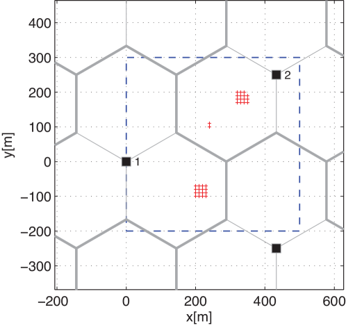
Figure 4: Example network topology. Base-stations are indicated by solid squares labelled 1,2 and 3, UEs by dots.

Figure 5 shows tilt angle time histories for the two base stations when using Algorithm 1. It can be seen that the tilt angles converge to the optimum in less than 600 iterations. Figure 6 shows the corresponding network sum-throughput vs time. Also shown in the network sum-throughput for fixed antenna angles of $8^{\circ}$. Optimising the tilt angles increases the network sum throughput by almost factor of 18 compared to the use of fixed angles. As already noted, the improvement is expected to be particularly pronounced in this simple example since the users are grouped into clusters, and so angling the antennas to point towards their respective clusters both greatly increases received power and decreases interference. We note that significant performance gains are, however, also observed in the more realistic scenario studied in Section VI and this reflects the fundamental importance of antenna tilt angle to network performance.

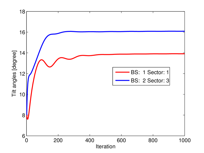
Figure 5: Tilt angle vs iteration number with Algorithm 1.

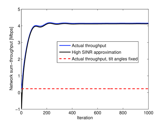
Figure 6: Normalised network sum-throughput vs iteration number with Algorithm 1. Here, the network sum-throughput is normalised by dividing by the number of users in the network.

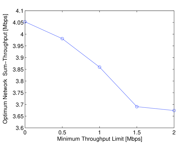
Figure 7: Normalised network sum-throughput as minimum throughput constraint $\underline{r}$ is varied. The network sum-throughput is normalised by dividing by the number of users in the network.

Fig 7 illustrates the impact of the minimum throughput constraint $\underline{r}$ on network sum-throughput. It can be seen that as $\underline{r}$ is increased from zero to 2Mbps, the network sum-throughput decreases but that the impact is minor. Note that as $\underline{r}$ is increased beyond 2Mbps the optimisation becomes infeasible as the stations at the cell edge are unable to support such high rates.

As discussed in Section IV-F, UE location information is used when calculating (20) in Algorithm 1. In practice this location information will be approximate in nature. Fig 8 plots the optimised network sum-throughput vs the standard deviation of the location error when zero-mean gaussian noise is added to the true user locations. It can be seen that, as might be expected, the optimised sum-throughput falls as the noise level is increased. However, the decrease is small (less than 5%) even for relatively large location errors.

Figure 8: Optimised network sum-throughput vs. magnitude of location error, error bars indicate the standard deviation for 100 runs of simulation for each point. The network sum-throughput is normalised by dividing by the number of users in the network.

V Any SINR: Proportional Fair Rate Allocation

In this section we relax the assumption of operation in the high SINR regime. However, this comes at the cost of restricting attention to proportional fair rate allocations. We consider the following utility fair optimisation problem (P2):

$$\max_{\Theta} \sum_{u\in{\mathcal{U}}}\log R_{u}(\Theta)$$ (28)

$$s.t.\quad \underline{\theta}\leq\theta_{b}\leq\bar{\theta},\quad b\in{\mathcal{B}}$$ (29)

$$\log\underline{r}\leq\log R_{u}(\Theta),\quad u\in{\mathcal{U}}$$ (30)

where $R_{u}(\Theta)$ is given by (6).

V-A Convexity Properties

We recall the following,

Lemma 4 ([15])

$h(x)=\log(\log(1+e^{x}))$ is concave and non-decreasing in $x\in\mathcal{R}$.

Turning now to $R_{u}(\Theta)$, we begin by observing that

Lemma 5

$\log(r_{u}(\Theta))$ is concave in $\Theta$.

Proof:

From (7) we have

$$\log(r_{u}(\Theta)) =\frac{w}{N_{sc}}\sum_{n=1}^{N_{sc}}\log(\log(1+\kappa\gamma_{u,n}(\Theta))$$ (31)

$$=\frac{w}{N_{sc}}\sum_{n=1}^{N_{sc}}\log(\log(1+e^{\hat{r}_{u,n}(\Theta)}))$$ (32)

where $\hat{r}_{u,n}(\Theta)=\log(\kappa\gamma_{u,n}(\Theta))$. That is, the mapping from vector $\Theta$ to $\log(r(\Theta))$ is the vector composition of $h(x)$ in Lemma 5 and $\hat{r}_{u,n}(\Theta)$. By Lemmas 1 and 2, $\hat{r}_{u,n}(\Theta)$ is concave in $\Theta$. By [12, p86], the vector composition a non-decreasing concave function and a concave function is concave. ∎

and

Theorem 3

$\log R_{u}(\Theta)$ is concave in $\Theta$.

Proof:

From (6) we have

$$\log R_{u}(\Theta) =\log\min\{\bar{r},r_{u}(\Theta)\}$$ (33)

$$\stackrel{{\scriptstyle(a)}}{{=}}\min\{\log\bar{r},\log r_{u}(\Theta)\}$$ (34)

where $(a)$ follows from the fact that the $\log$ function is monotonically increasing. By Lemma 5, $\log r_{u}(\Theta)$ is concave. Since the $\min$ function is concave non-decreasing, when composed with $\log r_{u}(\Theta)$ it is concave i.e. $\log\hat{R}_{u}(\Theta)$ is concave in $\Theta$. ∎

V-B Convex Optimisation

It follows from Theorem 3 that the objective of optimisation problem (P2) is concave. Constraints (29) are linear (so convex). The RHS of constraint (30) is concave, again by Theorem 3, and so this constraint is convex. It follows that optimisation problem (P2) is convex and a solution exists.

V-C Distributed Algorithm

The Slater condition is satisfied and strong duality holds. We can therefore apply a similar approach as in Section IV-E to develop a distributed algorithm for finding the optimal antenna tilt angles.

The Lagrangian is:

$$L(\Theta,\Lambda) = -\sum_{u\in{\mathcal{U}}}\log R_{u}(\Theta)+\sum_{u\in{\mathcal{U}}}\lambda_{u}^{1}(\log\underline{r}-\log R_{u}(\Theta))$$ (35)

$$\>+\sum_{b\in{\mathcal{B}}}\lambda^{2}_{b}(\underline{\theta}-\theta_{b})+\sum_{b\in{\mathcal{B}}}\lambda^{3}_{b}(\theta_{b}-\bar{\theta})$$

We can now apply Algorithm 1 to solve (P2) provided we use the appropriate gradients:

$$\partial_{\theta_{b}}L(\Theta,\Lambda) = -\sum_{u\in{\mathcal{U}}}\left(1+\lambda_{u}^{1}\right)\partial_{\theta_{b}}(\log{R}_{u}(\Theta))-\lambda^{2}_{b}+\lambda^{3}_{b}$$ (36)

$$\partial_{\lambda_{u}^{1}}L(\Theta,\Lambda) = \log\underline{r}-\log R_{u}(\Theta)$$ (37)

$$\partial_{\lambda_{b}^{2}}L(\Theta,\Lambda) = \underline{\theta}-\theta_{b}$$ (38)

$$\partial_{\lambda_{b}^{3}}L(\Theta,\Lambda) = \theta_{b}-\bar{\theta}$$ (39)

with
$\displaystyle\frac{\partial r_{u}}{\partial\theta_{b}}$ $\displaystyle=\begin{cases}\frac{\partial G_{v}(\theta_{b},d_{b,u})}{\partial\theta_{b}}\frac{\kappa H_{u}(\theta_{b(u)})}{\kappa H_{u}(\theta_{b(u)})+I_{u\in b(u)}}&b=b(u)\\ \frac{\partial\hat{G}_{v}(\theta_{b},d_{b,u})}{\partial\theta_{b}}\bigg{(}\frac{\hat{H}_{u}(\theta_{b(u)})}{\kappa H_{u}(\theta_{c})+I_{u\in{\mathcal{B}}\setminus\{b(u)\}}}-\frac{\hat{H}_{u}(\theta_{b(\acute{u})})}{I_{u\in{\mathcal{B}}\setminus\{b(u)\}}}\bigg{)}&b\neq b(u)\\ \end{cases}$ and

$$I_{u\in b(u)}=\sum_{c\in{\mathcal{B}}\setminus\{b(u)\}}\hat{H}_{u}(\theta_{c})+\eta_{u,n}$$ (40)

V-D Example

We revisit the example in section IV-G. Fig 9 compares the results for optimisation problems $(P1)$ and $(P2)$. Fig 9(a) shows the sum-throughput from Fig 6 and when solving proportional fair allocation problem $(P2)$. As expected, the sum throughput is lower for the proportional fair allocation. Fig 9(b) compares the sum-log-throughput. As expected, the sum-log-throughput is higher for the proportional fair allocation problem $(P2)$. Fig 10 shows detail of the throughputs assigned to individual users to maximise sum-throughput and for proportional fairness. It can be seen that the throughput assignments are broadly similar in both cases, with the primary difference being the throughputs assigned to the two users located at the cell edge (numbered 33 and 34 in Fig 10). The proportional fair allocation assigns significantly higher rate to these edge stations than does the max sum-throughput allocation.

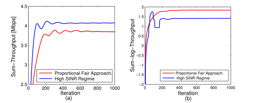
Figure 9: (a) Comparing normalised sum-throughput from Fig 6 and when solving proportional fair allocation problem $(P2)$ – as expected, the sum throughput is lower for the proportional fair allocation. (b) Comparing normalised sum-log-throughput – as expected, the sum-log-throughput is higher for the proportional fair allocation. In all cases the network throughput is normalised by dividing by the number of users in the network.

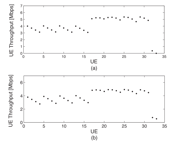
Figure 10: User throughput assignments for (a) sum-throughput maximisation in the high SINR regime and (b) proportional fair rate allocation.

VI Performance Evaluation

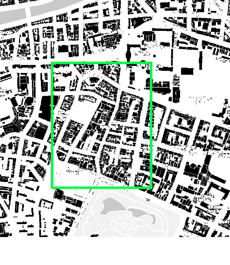
(a) Street map

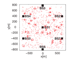
(b) User and base-station locations.

Figure 11: Dublin, Ireland example.

In this section we consider a realistic example based on data from the cellular network covering Grafton Street and Dawson Street in downtown Dublin, Ireland, see Fig 11a. These are major shopping streets close to the centre of Dublin city, with a large number of cellular users. We consider a section of the network with 21 sectors in a $1500m\times 1500m$ area and with an inter-site distance of $800m$. Environmental characteristics are derived from experimental measurement data with a combination of non-line of sight and line-of sight paths. Path loss and log-normal shadow fading parameters are derived from [11] for macro urban scenarios and detailed Table II. There are 1350 users, with locations as shown in Fig 11b. We focus on the performance experienced by the 388 users associated with the centre base station (indicated by BS1 in Fig 11b).

TABLE II: Dublin scenario simulation parameters

Dublin Scenario Simulation Parameters
Site and Sector	Inter-site distance	$800m$
Channel	NLOS exponential path loss factor	$3.9$
	NLOS fixed path loss factor	$10^{-2.1}$
	LOS exponential path loss factor	$2.2$
	LOS fixed path loss factor	$10^{-3.4}$
	Shadow fading standard deviation	$6$
	Shadow fading mean	$0$
Optimisation	Step size $\alpha$	$0.01$

Figures 12 shows the proportional fair rate allocation. For comparison, results are also shown when a fixed tilt angle of $8^{\circ}$ is used. It can be seen from Fig 12(a) that the sum-log-throughput objective function is improved by 22% by tilt angle optimisation, and that Algorithm 1 converges rapidly to the optimal allocation. From the cumulative distribution fucntion (CDF) in Fig 12(b) it can be seen the user throughputs are also significantly increased, with the median throughput increased by almost a factor of 4 compared to use of fixed angles.

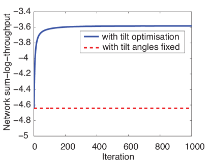
(a) Normalised Sum-log-throughput

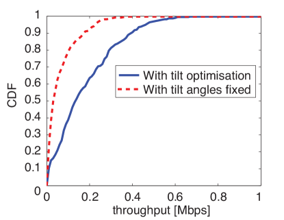
(b) CDF of user throughputs.

Figure 12: Proportional fair rate allocation, Dublin example. For comparison, results are also shown when a fixed tilt angle of $8^{\circ}$ is used (indicated by dashed lines).

VII LTE SIMO Links and MMSE Post-Processing

In this section we extend the performance evaluation to consider LTE SIMO links with one transmit antenna on the BS and two receive antennas at the UE. The presence of two antennas at the receiver allows the UE to cancel one interferer. Hence, if interference is dominated by a single transmitter then we expect the use of SIMO links will allow inter-cell interference to be significantly reduced. Our interest here is in the impact that this interference cancellation has on the size of throughput gain achievable by tilt angle adjustment.

We consider a SIMO link with linear Minimum Mean Square Error (LMMSE) post processing applied to the received signal to mitigate neighbouring cell interference. Defining channel vector $\textbf{k}_{u}=[k_{1}\ k_{2}]^{T}$, the channel gain for user $u$ is:

$$\textbf{k}_{u}=\sqrt{\frac{H_{u}(\theta_{b})}{P}}\sqrt{10^{S_{b,u}/10}}\textbf{q}_{b,u}.$$ (41)

where $S$ is a zero mean Gaussian random variable representing slow fading effects, $\textbf{q}_{b,u}$ is a Rayleigh flat fading vector and $P$ is the power of the transmitted signal assuming all base stations transmit at $P=P_{b,u}$. We can consider the elements of $\textbf{q}_{b,u}$ to be independent complex random Gaussian processes corresponding to the channels of base station $b$ and user $u$, provided that the antenna elements are sufficiently separated (typically on the order of half a wavelength apart). We identify the inter-cell interference vector $\textbf{v}_{u}=[v_{1}\ v_{2}]^{T}$ for user $u$ by the strongest interferer:

$$\textbf{v}_{u}=\sqrt{\max_{c\in{\mathcal{B}}\backslash\{b(u)\}}\{\hat{H}_{u}(\theta_{c})10^{S_{c,u}/10}\}}\textbf{q}_{c_{max},u}$$ (42)

The remaining inter-cell interference is modelled as spatially white Gaussian noise[16], which comprises the noise vector $\boldsymbol{n}_{u}=\begin{bmatrix}n_{1}\\ n_{2}\\ \end{bmatrix}$ where $n_{1}$ and $n_{2}$ are independent Gaussian variables:

$$N_{0}=E[n_{1}n_{1}^{H}]=E[n_{2}n_{2}^{H}]=\sum_{\shortstack{$\scriptstyle c\in{\mathcal{B}}\backslash\{b(u)\}$ \\ $\scriptstyle c\neq c_{max}$}}\hat{H}_{u}(\theta_{c})+\eta_{u}$$ (43)

Hence, the received signal (${\boldsymbol{y}}$) is given by:

$$\textbf{y}_{u}=\textbf{k}_{u}\textbf{x}+\textbf{v}_{u}+\textbf{n}_{u}$$ (44)

with $E[xx^{H}]=P$. The linear MMSE combining vector $\textbf{w}_{u}=[w_{1}\ w_{2}]^{T}$, is given by:

$$\textbf{w}_{u}=\textbf{k}_{u}^{H}{(\textbf{k}_{u}\textbf{k}_{u}^{H}+\frac{\boldsymbol{\Phi}+N_{0}\textbf{I}}{P})}^{-1}$$ (45)

where$\Phi$ is the autocorrelation of interference vector v:

$$\boldsymbol{\Phi}=E[\textbf{v}_{u}\textbf{v}_{u}^{H}]=\begin{bmatrix}|v_{1}|^{2}&v_{1}v_{2}^{H}\\ v_{2}v_{1}^{H}&|v_{2}|^{2}\\ \end{bmatrix}=\begin{bmatrix}\phi_{11}&\phi_{12}\\ \phi_{21}&\phi_{22}\\ \end{bmatrix}$$ (46)

By applying the MMSE weights on the received signal, the post processing SINR is calculated as:

$$\gamma_{u}^{MMSE}=$$

$$\frac{P|w_{1}k_{1}+w_{2}k_{2}|^{2}}{{|w_{1}|}^{2}\phi_{11}+{|w_{2}|}^{2}\phi_{22}+2Re\{w_{1}w_{2}^{H}\phi_{12}\}+N_{0}(|w_{1}|^{2}+|w_{2}|^{2})}$$ (47)

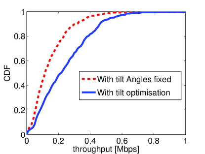
(a) with fast fading

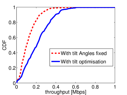
(b) without fast fading

Figure 13: User throughput CDFs with SIMO links and MMSE detection, Dublin example. Fast fading is modelled by generating $300$ samples using the 3GPP typical urban channel model, where the speed of the mobile user and carrier frequency are $3km/h$ and $2GHz$ respectively.

We average the post processing SINRs over the multipath fading samples. Using the averaged post processing SINRs, user throughputs with and without tilt optimisation can be calculated using (6).

Fig 13 shows CDF of the user throughputs for SIMO links with MMSE detection, with and without flat fading. As expected, the use of MMSE detection yields significant improvements in the user throughputs. The throughput gains achieved by tilt optimisation can be compared for SISO links and for SIMO links with an optimal LMMSE detector by comparing Figs 12b and 13. The gain in the mean user throughput achieved by tilt optimisation is decreased from $83.07\%$ to $67.42\%$ when MMSE detection is employed. However, the gain in the log-sum-rate (which is the objective function of optimisation ${P2}$) only changes from $22.29\%$ to $22.00\%$. That is, while MMSE detection enhances inter-cell interference mitigation, tilt optimisation can still yield significant improvements in network capacity.

We can investigate this behaviour in more detail as follows. Let

$$\epsilon_{u}=\frac{\max_{c\in{\mathcal{B}}\backslash\{b(u)\}}\{\hat{H}_{u}(\theta_{c})10^{S_{c,u}/10}\}}{\sum_{c\in{\mathcal{B}}\backslash\{b(u)\}}\hat{H}_{u}(\theta_{c})10^{S_{c,u}/10}}$$ (48)

be the ratio of the largest interferer to the total interference experienced by a user $u$. The CDF of $\epsilon$ for the Dublin example is shown in Fig 14(a). It can be seen that approximately 40% of users have $\epsilon$ values less than 0.5 i.e. for 40% of users the the strongest interferer power is less than the sum of the power of the other interferers. Fig 14(b) shows the corresponding spatial distribution of $\epsilon$. It can be seen that the strongest interferer is dominant at the edge of antenna sectors and along the nulls of the sector antennas. However, the intensity of the strongest interferer decreases along the edges of the base station coverage area and alongside the antennas. Table III details the throughput gains achieved by tilt angle optimisation for both SISO and SIMO links and for users with different $\epsilon$ ratios. It can be seen that the throughput gain obtained by tilt angle optimisation for users with $\epsilon>.5$ is reduced when SIMO links are used. However, the gain is similar for both SISO and SIMO links for users with $\epsilon\leq.5$, once MMSE post processing is applied, and as noted above this consists of approximately 40% of users.

In summary, although the mean user throughput is improved for both fixed and optimal tilt angles for SIMO links with MMSE, tilt optimisation can still yield considerable performance gains.

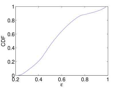
(a)

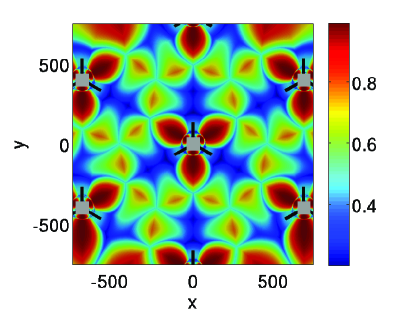
(b)

Figure 14: Contribution of the strongest interference to the total Interference: (a) cumulative distributed function of $\epsilon$ in the central BS coverage area. (b) Distribution of $\epsilon$ relative to the user positions.

TABLE III: User throughput gains due to tilt angle optimisation for both SISO and SIMO links and vs $\epsilon$, Dublin example.

	Mean Throughput Gain [%]
	SISO	SIMO & MMSE Detection
$0\leq\epsilon_{u}\leq.5$	$54.5$	$52.3$
$.5<\epsilon_{u}\leq.8$	$128$	$85.99$
$.8<\epsilon_{u}\leq 1$	$147$	$91.99$
$0\leq\epsilon_{u}\leq 1$	$83.07$	$67.42$

VIII Conclusions and Future Work

VIII-A Conclusions

In this paper we formulate adaptation of antenna tilt angle as a utility fair optimisation task. Namely, the objective is to jointly adjust antenna tilt angles within the cellular network so as to maximise user utility, subject to network constraints. Adjustments at base stations must be carried out jointly in a coordinated manner in order to manage interference. This optimisation problem is non-convex, but we show that under certain conditions it can be reformulated as a convex optimisation. Specifically, we show that (i) in the high SINR operating regime and with an appropriate choice of variables the optimisation is convex for any concave utility function, and (ii) in any SINR regime the optimisation can be formulated in a convex manner when the objective is a proportional fair rate allocation. Since the optimisation is not well-suited to use of standard dual methods, we develop a primal-dual method for finding the optimal antenna tilt angles. This approach is lightweight, making use of measurements which are already available at base stations, and suited to distributed implementation. The effectiveness of the proposed approach is demonstrated using a number of simulation examples, including a realistic example based on the cellular network in Dublin, Ireland, and is found to yield considerable performance gains.

Appendix: Optimisation Problem

Consider the optimisation problem

$$\min_{\mathbf{x}}f(\mathbf{x})\qquad s.t.\quad g_{i}(\mathbf{x})\leq 0,\quad i=1,\cdots,m$$

with $\mathbf{x}\in\mathcal{R}^{n}$, $f(\mathbf{x}):\mathcal{R}^{n}\rightarrow\mathcal{R}$ convex, $g_{i}(\mathbf{x}):\mathcal{R}^{n}\rightarrow\mathcal{R}$, $i=1,\cdots,m$ convex. For simplicity we will assume that $f(\mathbf{x})$, $g_{i}(\mathbf{x})$ are differentiable, but this could be relaxed. The optimisation problem is convex and so at least one solution exists, let $X^{*}$ denote the set of solutions Assuming the Slater condition is satisfied, then strong duality holds and the KKT conditions are necessary and sufficient for optimality. The Lagrangian is

$$L(\mathbf{x},\mathbf{u})=f(\mathbf{x})+\sum_{i=1}^{m}u_{i}g_{i}(\mathbf{x})$$

where $u_{i}$ is the multiplier associated with constraint $g_{i}(\mathbf{x})\geq 0$ and $\mathbf{u}=(u_{1},\cdots,u_{m})$. At an optimum $\mathbf{x}^{*}\in X^{*}$, the multipliers must lie in set $U(\mathbf{x}^{*})=\{\mathbf{u}:\mathbf{u}=\arg\sup_{\mathbf{u}\geq 0}L(\mathbf{x}^{*},\mathbf{u})\}$.

VIII-B Gradient Algorithm

We consider the following primal-dual update

$$x_{j}(t+1) = x_{j}(t)-\alpha\partial_{x_{j}}L(\mathbf{x}(t),\mathbf{u}(t)),\quad j=1,\cdots,n$$ (49)

$$u_{i}(t+1) = \left[u_{i}(t)+\alpha\partial_{u_{i}}L(\mathbf{x}(t),\mathbf{u}(t))\right]^{+},\quad i=1,\cdots,m$$ (50)

where step size $\alpha>0$ and $\partial_{x_{j}}L(\mathbf{x},\mathbf{u})$, $\partial_{u_{i}}L(\mathbf{x}(t),\mathbf{u}(t))$ are subgradients of $L(\mathbf{x}(t),\mathbf{u}(t))$ with respect to $x_{j}$ and $u_{i}$ respectively. We have $\partial_{x_{j}}L(\mathbf{x},\mathbf{u})=\partial_{x_{j}}f(\mathbf{x})+\sum_{i=1}^{m}u_{i}\partial_{x_{j}}g_{i}(\mathbf{x})$ and $\partial_{u_{i}}L(\mathbf{x}(t),\mathbf{u}(t))=g_{i}(\mathbf{x})$ with $\partial_{x_{j}}f(\mathbf{x})$ a subgradient of $f(\mathbf{x})$ with respect to $x_{j}$, $\partial_{x_{j}}g_{i}(\mathbf{x})$ a subgradient of $g_{i}(\mathbf{x})$ with respect to $x_{j}$. Projection $[z]^{+}=z$ when $z\geq 0$, $0$ otherwise.

VIII-C Fixed Points

Lemma 6 (Fixed points)

$(\mathbf{x}^{*},\mathbf{u}^{*})$ with $\mathbf{x}^{*}\in X^{*}$, $\mathbf{u}^{*}\in U(\mathbf{x}^{*})$ is a fixed point of the dynamics (49)-(50).

Proof:

From the KKT conditions, $\partial_{x_{j}}L(\mathbf{x}^{*},\mathbf{u}^{*})=0$ and so $(\mathbf{x}^{*},\mathbf{u}^{*})$ is a fixed point of (49). Since $(\mathbf{x}^{*},\mathbf{u}^{*})$ is feasible, $\partial_{u_{i}}L(\mathbf{x}^{*},\mathbf{u}^{*})=g_{i}(\mathbf{x}^{*})\leq 0$. We need to consider two cases: (i) $\partial_{u_{i}}L(\mathbf{x}^{*},\mathbf{u}^{*})=0$ in which case $(\mathbf{x}^{*},\mathbf{u}^{*})$ is a fixed point of (50) and (ii) $\partial_{u_{i}}L(\mathbf{x}^{*},\mathbf{u}^{*})<0$ in which case by complementary slackness $u_{i}^{*}=0$ and this is also a fixed point of (50). Hence, every $(\mathbf{x}^{*},\mathbf{u}^{*})$ is a fixed point of the dynamics (49)-(50). ∎

VIII-D Convergence

Let $V(\mathbf{x},\mathbf{u}):=\min_{\mathbf{x}^{*}\in X^{*},\mathbf{u}^{*}\in U(\mathbf{x}^{*})}\sum_{j=1}^{n}(x_{j}-x_{j}^{*})^{2}+\sum_{i=1}^{m}(u_{i}-u_{i}^{*})^{2}$. Observe that (i) $V(\mathbf{x},\mathbf{u})\geq 0$ and (ii) $V(\mathbf{x},\mathbf{u})=0$ if and only if $\mathbf{x}\in X^{*}$ and $\mathbf{u}\in U(\mathbf{x}^{*})$.

Lemma 7

Under update (49)-(50),

$$V(\mathbf{x}(t+1),\mathbf{u}(t+1))\leq$$

$$\bigg{[}V(\mathbf{x}(t),\mathbf{u}(t))-2\alpha\left(L(\mathbf{x}(t),\mathbf{u}^{*}(t))-L(\mathbf{x}^{*}(t),\mathbf{u}(t))\right)$$

$$\quad\>+\alpha^{2}(t)\epsilon(\mathbf{x}(t),\mathbf{u}(t))\bigg{]}$$

where $\epsilon(\mathbf{x},\mathbf{u})=\sum_{j=1}^{n}\left(\partial_{x_{j}}L(\mathbf{x},\mathbf{u})\right)^{2}+\sum_{i=1}^{m}g_{i}^{2}(\mathbf{x})$ and $(\mathbf{x}^{*}(t),\mathbf{u}^{*}(t))=\arg\min_{\mathbf{x}^{*}\in X^{*},\mathbf{u}^{*}\in U(\mathbf{x}^{*})}\sum_{j=1}^{n}(x_{j}(t)-x_{j}^{*})^{2}+\sum_{i=1}^{m}(u_{i}(t)-u_{i}^{*})^{2}$.

Proof:

From (49), for any $x^{*}\in X^{*}$ we have

$$\sum_{j=1}^{n}\left(x_{j}(t+1)-x_{j}^{*}\right)^{2}$$

$$=\sum_{j=1}^{n}\left(x_{j}(t)-x_{j}^{*}-\alpha\partial_{x_{j}}L(\mathbf{x}(t),\mathbf{u}(t))\right)^{2}$$

$$=\sum_{j=1}^{n}(x_{j}(t)-x_{j}^{*})^{2}+2\alpha\sum_{j=1}^{n}(x_{j}^{*}-x_{j}(t))\partial_{x_{j}}L(\mathbf{x}(t),\mathbf{u}(t))$$

$$\quad\>+\alpha^{2}(t)\sum_{j=1}^{n}\left(\partial_{x_{j}}L(\mathbf{x}(t),\mathbf{u}(t))\right)^{2}$$

$$\stackrel{{\scriptstyle(a)}}{{\leq}}\sum_{j=1}^{n}(x_{j}(t)-x_{j}^{*})^{2}+2\alpha\left(L(\mathbf{x}^{*},\mathbf{u}(t))-L(\mathbf{x}(t),\mathbf{u}(t))\right)$$

$$\quad\>+\alpha^{2}(t)\sum_{j=1}^{n}\left(\partial_{x_{j}}L(\mathbf{x}(t),\mathbf{u}(t))\right)^{2}$$ (51)

where $(a)$ follows from the fact that $L(\mathbf{x}^{*},\mathbf{u})-L(\mathbf{x},\mathbf{u})\geq\sum_{j=1}^{n}\left(x_{j}^{*}-x_{j}\right)\partial_{x_{j}}L(\mathbf{x},\mathbf{u})$ (from the definition of a subgradient). From (50) we have for any $\mathbf{u}^{*}\in U(\mathbf{x}^{*})$ that

$$\sum_{i=1}^{m}\left(u_{i}(t+1)-u_{i}^{*}\right)^{2}=\sum_{i=1}^{m}\left(u_{i}(t)+\alpha g_{i}(\mathbf{x}(t))-u_{i}^{*}\right)^{2}$$

$$\qquad=\sum_{i=1}^{m}\left(u_{i}(t)-u_{i}^{*}\right)^{2}$$

$$\qquad\qquad+2\alpha\sum_{i=1}^{m}\bigg{(}(u_{i}(t)-u_{i}^{*})g_{i}(\mathbf{x}(t))+\alpha^{2}(t)g_{i}^{2}(\mathbf{x}(t))\bigg{)}$$

$$\qquad\stackrel{{\scriptstyle(a)}}{{=}}\sum_{i=1}^{m}\left(u_{i}(t)-u_{i}^{*}\right)^{2}+2\alpha\left(L(\mathbf{x}(t),\mathbf{u}(t))-L(\mathbf{x}(t),\mathbf{u}^{*})\right)$$

$$\qquad\qquad+\alpha^{2}(t)g_{i}^{2}(\mathbf{x}(t))$$ (52)

where $(a)$ follows from the observation that

$$L(\mathbf{x},\mathbf{u})-L(\mathbf{x},\mathbf{u}^{*}) = f(\mathbf{x})+\sum_{i=1}^{m}u_{i}g_{i}(\mathbf{x})-f(\mathbf{x})-\sum_{i=1}^{m}u_{i}^{*}g_{i}(\mathbf{x})$$

$$= \sum_{i=1}^{m}(u_{i}-u_{i}^{*})g_{i}(\mathbf{x})$$

Then, from (51) and (52),

$$V_{\mathbf{u}^{*}}(\mathbf{x}(t+1),\mathbf{u}(t+1))$$

$$\quad\leq\sum_{j=1}^{n}(x_{j}(t+1)-x_{j}^{*}(t))^{2}+\sum_{i=1}^{m}(u_{i}(t+1)-u_{i}^{*}(t))^{2}$$

$$\quad\leq V_{\mathbf{u}^{*}}(\mathbf{x}(t),\mathbf{u}(t))-2\alpha\left(L(\mathbf{x}(t),\mathbf{u}^{*}(t))-L(\mathbf{x}^{*}(t),\mathbf{u}(t))\right)$$

$$\qquad\quad+\alpha^{2}(t)\epsilon(\mathbf{x}(t),\mathbf{u}(t))$$

∎

Lemma 8

Under update (49)-(50), when $\frac{1}{t}\sum_{\tau=0}^{t}\epsilon(\mathbf{x}(\tau),\mathbf{u}(\tau))\leq M$ (e.g. this holds when $(\mathbf{x}(\tau),\mathbf{u}(\tau))$ is bounded and $f(\mathbf{x})$, $g(\mathbf{x})$ are continuous) we have

$$0 \leq \frac{1}{t}\sum_{\tau=0}^{t}\left(L(\mathbf{x}(\tau),\mathbf{u}^{*}(\tau))-L(\mathbf{x}^{*}(\tau),\mathbf{u}(\tau))\right)$$

$$\leq \frac{1}{2\alpha t}V(\mathbf{x}(0),\mathbf{u}(0))+\frac{\alpha M}{2}$$

where $\mathbf{x}^{*}(\tau)\in X^{*}$ and $\mathbf{u}^{*}(\tau)\in U^{*}(\mathbf{x}^{*}(\tau))$.

Proof:

By Lemma 7,

$$V(\mathbf{x}(t+1),\mathbf{u}(t+1))-V(\mathbf{x}(0),\mathbf{u}(0))$$

$$\qquad\leq\sum_{\tau=0}^{t}\Big{(}-2\alpha\big{(}L(\mathbf{x}(\tau),\mathbf{u}^{*}(\tau))-L(\mathbf{x}^{*}(\tau),\mathbf{u}(\tau))\big{)}$$

$$\qquad\qquad\qquad\qquad+\alpha^{2}(t)\epsilon(\mathbf{x}(\tau),\mathbf{u}(\tau))\Big{)}$$

Hence,

$$\frac{1}{t}\sum_{\tau=0}^{t}\left(L(\mathbf{x}(\tau),\mathbf{u}^{*}(\tau))-L(\mathbf{x}^{*}(\tau),\mathbf{u}(\tau))\right)$$

$$\qquad\leq\frac{1}{2\alpha t}V(\mathbf{x}(0),\mathbf{u}(0))+\frac{\alpha}{2t}\sum_{\tau=0}^{t}\epsilon(\mathbf{x}(\tau),\mathbf{u}(\tau))$$

For $x^{*}\in X^{*}$, $\mathbf{u}^{*}\in U(\mathbf{x}^{*})$ recall $\mathbf{u}^{*}=\arg\sup_{\mathbf{u}\geq 0}L(\mathbf{x}^{*},\mathbf{u})$ and $\mathbf{x}^{*}=\arg\inf_{\mathbf{x}}L(\mathbf{x},\mathbf{u}^{*})$. Hence, $L(\mathbf{x}^{*},\mathbf{u})\leq L(\mathbf{x}^{*},\mathbf{u}^{*})\leq L(\mathbf{x},\mathbf{u}^{*})$ and $L(\mathbf{x},\mathbf{u}^{*})-L(\mathbf{x}^{*},\mathbf{u})\geq 0$. Therefore, $L(\mathbf{x}(\tau),\mathbf{u}^{*}(\tau))-L(\mathbf{x}^{*},\mathbf{u}(\tau))\geq 0$. Substituting for $\frac{1}{t}\sum_{\tau=0}^{t}\epsilon(\mathbf{x}(\tau),\mathbf{u}(\tau))\leq M$ then yields the result. ∎

Bahar Partov is pursuing a PhD degree at Hamilton Institute together with Bell-labs Alcatel-Lucent Ireland. She received her master’s degree from University of Essex at 2009. She did her undergraduate degree at University of Tabriz, Iran. Her current research interests are distributed algorithms for self-organized networks.

Doug Leith graduated from the University of Glasgow in 1986 and was awarded his PhD, also from the University of Glasgow, in 1989. In 2001, Prof. Leith moved to the National University of Ireland, Maynooth to assume the position of SFI Principal Investigator and to establish the Hamilton Institute (www.hamilton.ie) of which he is Director. His current research interests include the analysis and design of network congestion control and resource allocation in wireless networks.

Rouzbeh Razavi is a member of technical staff in the Autonomous Networks and Systems Research Department at Alcatel-Lucent Bell Labs Ireland and United Kingdom. He received his B.Sc. degree in electrical and electronics engineering from Khajeh Nasir Toosi University of Technology, Tehran, Iran. He also received a master’s degree with distinction in telecommunication and information systems and a Ph.D. in real time multimedia communication over wireless networks, both from the University of Essex, United Kingdom. At Bell Labs, Dr. Razavi’s current research work involves developing algorithms for large scale, distributed, self-organizing networks for the next generation of wireless networks (4G and beyond) and small cell flat cellular networks. He has published more than 42 technical papers in peer reviewed journals and conferences and has authored five book chapters.

References

- [1] I. Forkel, A. Kemper, R. Pabst, and R. Hermans, “The effect of electrical and mechanical antenna down-tilting in umts networks,” in 3G Mobile Communication Technologies, 2002. Third International Conference on (Conf. Publ. No. 489), pp. 86–90, IET, 2002.
- [2] F. Athley and M. Johansson, “Impact of electrical and mechanical antenna tilt on lte downlink system performance,” in Vehicular Technology Conference (VTC 2010-Spring), 2010 IEEE 71st, pp. 1–5, IEEE, 2010.
- [3] LTE; Evolved Universal Terrestrial Radio Access (E-UTRA); Self-configurating , Self-optimizating Network (SON); use cases and solutions; 3GPPTR 36.902 (Release 9), 2010.
- [4] E. Benner and A. Sesay, “Effects of antenna height, antenna gain, and pattern downtilting for cellular mobile radio,” Vehicular Technology, IEEE Transactions on, vol. 45, no. 2, pp. 217–224, 1996.
- [5] O. Yilmaz, S. Hamalainen, and J. Hamalainen, “Analysis of antenna parameter optimization space for 3gpp lte,” in Vehicular Technology Conference Fall (VTC 2009-Fall), 2009 IEEE 70th, pp. 1–5, IEEE, 2009.
- [6] H. Eckhardt, S. Klein, and M. Gruber, “Vertical antenna tilt optimization for lte base stations.,” in VTC Spring, pp. 1–5, IEEE, 2011.
- [7] R. Razavi, S. Klein, and H. Claussen, “A fuzzy reinforcement learning approach for self optimization of coverage in lte networks,” Bell Lab. Tech. J., vol. 15, pp. 153–175, Dec. 2010.
- [8] A. Temesváry, “Self-configuration of antenna tilt and power for plug & play deployed cellular networks,” in Wireless Communications and Networking Conference, 2009. WCNC 2009. IEEE, pp. 1–6, IEEE, 2009.
- [9] G. Calcev and M. Dillon, “Antenna tilt control in cdma networks,” in Proceedings of the 2nd annual international workshop on Wireless internet, p. 25, ACM, 2006.
- [10] A. Eisenblatter and H. Geerdes, “Capacity optimization for umts: Bounds and benchmarks for interference reduction,” in Personal, Indoor and Mobile Radio Communications, 2008. PIMRC 2008. IEEE 19th International Symposium on, pp. 1–6, IEEE, 2008.
- [11] 3rd Generation Partnership Project; Technical Specification Group Radio Access Network; Evolved Universal Terrestrial Radio Access (E-UTRA); Further advancements for E-UTRA physical layer aspects (Release 9), 2010.
- [12] S. Boyd and L. Vandenberghe, Convex optimization. Cambridge university press, 2004.
- [13] FCC, “Wireless E911 Location Accuracy Requirements.” http://www.fcc.gov/document/wireless-e911-location-accuracy-requirements-1/, 2011.
- [14] LTE; Evolved Universal Terrestrial Radio Access (E-UTRA); LTE Positioning Protocol (LPP); 3GPP TS 36.355 (Release 9), 2010-02.
- [15] J. Papandriopoulos, S. Dey, and J. Evans, “Optimal and distributed protocols for cross-layer design of physical and transport layers in manets,” IEEE/ACM Transactions on Networking (TON), vol. 16, no. 6, pp. 1392–1405, 2008.
- [16] Universal Mobile Telecommu nications System (UMTS); Spatial channel model for Multiple Input Multiple Output (MIMO) simulations (Release 11), 2012.