Algorithmic Aspects of Switch Cographs

Abstract

This paper introduces the notion of involution module, the first generalization of the modular decomposition of 2-structure which has a unique linear-sized decomposition tree. We derive an $\mathcal{O}(n^{2})$ decomposition algorithm and we take advantage of the involution modular decomposition tree to state several algorithmic results. Cographs are the graphs that are totally decomposable w.r.t modular decomposition. In a similar way, we introduce the class of switch cographs, the class of graphs that are totally decomposable w.r.t involution modular decomposition. This class generalizes the class of cographs and is exactly the class of (Bull, Gem, Co-Gem, $C_{5}$)-free graphs. We use our new decomposition tool to design three practical algorithms for the maximum cut, vertex cover and vertex separator problems. The complexity of these problems was still unknown for this class of graphs. This paper also improves the complexity of the maximum clique, the maximum independant set, the chromatic number and the maximum clique cover problems by giving efficient algorithms, thanks to the decomposition tree. Eventually, we show that this class of graphs has Clique-Width at most 4 and that a Clique-Width expression can be computed in linear time.

Introduction

Modular decomposition has arisen in different contexts as a very natural operation on many discrete structures such as graphs, directed graphs, 2-structures, automata, boolean functions, hypergraphs, or matroids. In graph theory, the study of modular decomposition as a graph decomposition technique was first introduced by Gallaï [16]. This notion has led to state several important properties of both structural and algorithmic flavour. Many graph classes such as cographs, $P_{4}$-sparse graphs or $P_{4}$-tidy graphs are characterized by the properties of their modular decomposition (see for example [2]).

Also, several classical graph problems (NP-complete in the general case) can be solved in polynomial time when restricted to classes of graphs that are “decomposable enough”. For example, [9, 22] designed efficient algorithms for the class of cographs which rely on the modular decomposition tree of the cographs.

We start from a generalization of modular decomposition, namely the umodular decomposition defined in [5]. In his PhD thesis[4], Bui Xuan has shown that the family of umodules of more general combinatorial objects (such as 2-structures [14]) has no polynomial-sized tree representation. Therefore, as far as we know, there is no generalization of modular decomposition that have a polynomial-sized tree representation in a more general context than graphs.

In this paper, we introduce the notion of involution modules, which is a generalization of modules but a restriction of umodules, and we show that the family of involution modules of any 2-structure has very strong properties. These properties are similar to the properties of modules, and lead us to derive in $\mathcal{O}(n^{2})$ time a unique linear-sized decomposition tree for any 2-structure. To this aim we use a very interesting switch operator that generalizes to 2-structures the well-known Seidel Switch introduced by [23] and widely studied by [19, 21, 18].

Then we focus our study on the particular case of 2-structure with two colors, namely undirected graphs which are more concerned by the algorithmic aspects than 2-structures. We consider the class of graphs totally decomposable with respect to the involution modular decomposition. We call this class the class of Switch Cographs and we show that switch cographs are exactly the graphs with no induced Gem, Co-Gem, $C_{5}$ nor Bull subgraphs. This graphs family is already known in the litterature (see for example [19]) and generalizes the widely studied class of cographs. Like the modular decomposition for cographs, the involution modular decomposition provides crucial algorithmic properties for the class of switch cographs. Using our decomposition approach we give efficient and practical algorithms for the class of switch cographs to well-known graph problems (NP-complete in the general case), namely the maximum cut and the vertex separator problems. The complexity of these problems was still unknown for this class of graphs. Since the Clique-Width of the switch cographs is bounded, the complexity of several graph problems depended on the celebrated Courcelle’s theorem. The theorem implies in particular that the maximum clique, the maximum independant set, the chromatic number the vertex cover and the minimum clique cover problems can be solved in polynomial time for the class of Switch Cographs. Nevertheless, the theorem induces a huge constant factor in the big-O notation and cannot be considered of practical interest. We then show that the involution modular decomposition tree can be used in order to derive a Clique-Width expression in linear time leading to a linear-time complexity for these problems. Then, we give easily implementable algorithms which ensure the same optimal complexity. Finally, we conclude this paper by showing that this class of graphs is strictly included in the class of graphs with Clique-width at most 4.

The paper is organized as follows, section 1 recalls definitions and the general framework of modular decomposition, section 2 introduces the notion of involution modules, studies its properties and presents the decomposition algorithm. Section 3 is devoted to the study of switch cographs and to the algorithms we designed thanks to the involution modular decomposition. Eventually, we discuss the noteworthy outcomes and open questions that follow from our work.

1 Definitions

We recall some definitions about generalisations of modular decomposition (as they are given in [5]). Let $X$ be a finite set. We say that two subsets $A,B\subseteq X$ are overlapping if the sets $A\cap B$, $A\setminus B$, $B\setminus A$ are not empty. Finally, we say that two sets $A,B\subseteq X$ are crossing if they are overlapping and $X\neq A\cup B$.é

Definition 1.1.

[14] 2-structure. A 2-structure $G$ is a couple $(X,E)$ where $X$ is a finite set (the set of the vertices) and $E$ is a function, $E:X^{2}\rightarrow\mathds{N}$.

We say that a 2-structure $G$ is symmetric if for all $x,y\in X$, $E(x,y)=E(y,x)$. An edge over $X$ is a pair $(x,y)$, $x,y\in X$ and $x\neq y$ and let $E_{2}(X)$ denotes the set of all edges over $X$. Throughout this paper, we only consider symmetric 2-structures and we always omit the word “symmetric”. For a given 2-structure $G=(X,E)$ we say that the set $C=\{i$ $|$ $\exists u,v$ s.t $E(u,v)=i\}$ is the set of the colors of the 2-structure. By $N^{i}_{s}(X^{\prime})$ we denote the set $\{x$ $|$ $x\in X^{\prime}$ and $E(s,x)=i\}$, basically the set of elements in $X^{\prime}$ that are connected to $s$ with the color $i$.

The reader may remark that any undirected graph is basically a 2-structure with 2 colors. Let us recall below the usual notation of modular decomposition.

1.1 Homogeneous Relation, Modules and Umodules

We now recall the notion of module for a 2-structure.

Definition 1.2.

[13] Modules. Let $G=(X,E)$ be a 2-structure. A subset $M\subseteq X$ is a module of $G$ if :

$\forall m$, $m^{\prime}\in M$, $\forall i\in C$, $N_{m}^{i}(X\setminus M)=N_{m^{\prime}}^{i}(X\setminus M)$.

We say that a module $M$ is trivial if $|M|$ $\leq$ $1$ or $M=X$. We now present the primary properties of modular decomposition. Throughout this section, we denote by $2^{X}$ the family of subsets of any finite set $X$.

Definition 1.3.

Partitive family. Let $X$ be a set of elements. $\mathcal{F}\subseteq 2^{X}$ is a partitive family if $X$ and $\emptyset$ $\in\mathcal{F}$ and for any overlapping sets $A$, $B\in\mathcal{F}$, $A\cap B\neq\emptyset$ and $A\cup B\neq X$ implies $A\cap B\in\mathcal{F}$, $A\cup B\in\mathcal{F}$, $A\setminus B\in\mathcal{F}$ and $A\bigtriangleup B\in\mathcal{F}$.

[7] showed that the family of modules of any graph (i.e 2-structure with two colors) is a partitive family and demonstrated the following theorem of particular importance.

Theorem 1.1.

[7] Decomposition theorem of partitive families. If $F$ is a partitive family, there exists a unique rooted undirected tree-representation of $F$, $\mathcal{T}(F)$, of size $\mathcal{O}(|X|)$. This tree representation is such that the internal nodes of $\mathcal{T}(F)$ can be labelled complete or prime such that:

• The leaves are exactly the elements of $X$;

• Let $N$ be a node with $k$ siblings $N_{1},...,N_{k}$,

  If $N$ is a complete node, for any $I\subset\{1,...,k\}$ such that $1<|I|<k$, $\bigcup\limits_{i\in I}X_{i}\in F$, and

  if $N$ is a prime node, for any element $i\in\{1,...,k\}$, $X_{i}\in F$,
  where $X_{i}$ is the set of elements of leaves whose paths to $N$ traverse $N_{i}$;

• There are no more sets in $F$ than the ones described above.

[13] presented an $\mathcal{O}(|X|^{2})$ algorithm which computes the tree-decomposition of the family of modules of any 2-structure. We conclude this section by reminding a generalization of modular decomposition introduced by [5].

Definition 1.4.

Umodules. Let $G=(X,E)$ be a 2-structure. A subset $U$ of $X$ is a umodule if $\forall u,u^{\prime}\in U,$ $\forall x,x^{\prime}\in X\backslash U$,

$\exists i\in C$, $x\in N_{u}^{i}$ and $x^{\prime}\notin N_{u}^{i}$ $\iff$ $\forall j\in C$, $x\in N_{u}^{j}$ and $x^{\prime}\notin N_{u}^{j}$

This led [5] to introduce the notion of partitive crossing family, namely :

Definition 1.5.

Partitive crossing family. Let $X$ be a set of elements. $\mathcal{F}\subseteq 2^{X}$ is a partitive crossing family if $X$ and $\emptyset$ $\in\mathcal{F}$ and for any crossing sets $A$, $B\in\mathcal{F}$, $A\cap B\neq\emptyset$ and $A\cup B\neq X$ implies $A\cap B\in\mathcal{F}$, $A\cup B\in\mathcal{F}$, $A\setminus B\in\mathcal{F}$ and $A\bigtriangleup B\in\mathcal{F}$.

Then [5] showed that the family of umodules of a graph is a partitive crossing family.

Theorem 1.2.

[6] Decomposition theorem partitive crossing families. If $\mathcal{F}$ is a partitive crossing family, there exists a unique unrooted and directed tree-representation of $\mathcal{F}$, $\mathcal{T}(\mathcal{F})$, of size $\mathcal{O}(|X|)$. This tree-representation is such that the nodes of $\mathcal{T}(\mathcal{F})$ can be labelled complete or prime. such that:

• For any nodes $N_{1},N_{2}$, if $(N_{1},N_{2})$ is an arc of the tree then $N_{1}$ is in the family.

• If $N$ is a node with $k$ in-neighbors $N_{1},...,N_{k}$ :

  If $N$ is a complete node, for any $I\subset\{1,...,k\}$ such that $1<|I|<k$, $\bigcup\limits_{i\in I}X_{i}\in F$, and

  if $N$ is a prime node, for any element $i\in\{1,...,k\}$, $X_{i}\in F$,
  where $X_{i}$ is the set of leaves whose paths to $N$ traverse $N_{i}$.

• There are no more sets in $F$ than the ones described above.

[5] presented an algorithm which computes for any graph $G=(X,E)$ the tree representation of its family of umodules with an $\mathcal{O}(|X|+|E|)$ complexity.

Figure 1: The sets $\{a,c,e\}$ and $\{a,d,e\}$ are crossing umodules but their intersection, $\{a,e\}$ is not a umodule.

2 Involution Modules, a New Decomposition Tool

2.1 Discussion

The notion of umodule presented above and due to [5, 11] induces a family which has strong properties of both algorithmic and structural flavour on graphs. Nevertheless, unlike the modules, the family of umodules of a 2-structure has no polynomial-sized tree-representation and so cannot be used in order to decompose more general objects such as 2-structures [4].

For example, figure 1 shows that there exists a 2-structure with only 3 colors whose family of umodules is not closed under intersection. We found two other 2-structures with 3 colors whose families of umodules are not closed under difference and symmetric difference. Eventually, [4] showed that the family of umodules of any 2-structure can not be represented in polynomial time. We introduce below the notion of involution module, a generalization of modules and a restriction of umodules. We show that the family of involution modules of any 2-structure has similar properties as the family of modules, namely the closure under union, intersection, difference and symmetric difference of crossing sets. These properties lead to a unique linear-sized tree-representation by theorem 1.2 and allow us to derive an optimal algorithm that computes it.

2.2 Definition and Properties

Definition 2.1.

Involution Modules. Let $G=(X,E)$ be a 2-structure, $\mathcal{I}$ an involution of the colors without fix point. $U\subset X$ is an involution module if, for all $u,v\in U$,

• Either, $\forall i\in\{1,...,|C|\}$, $N_{s}^{i}(X\backslash U)=N_{u}^{\mathcal{I}(i)}(X\backslash U)$.

• Or, $\forall i\in\{1,...,|C|\}$, $N_{s}^{i}(X\backslash U)=N_{u}^{i}(X\backslash U)$.

Remark like elements of a umodule, elements of the involution module have to partition the rest of the 2-structure in the same way.

Throughout this paper we will consider involutions without fix point. Figure 2 shows how an involution module is connected to the rest of the 2-structure.

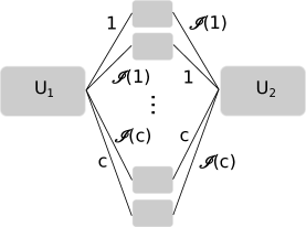
Figure 2: An involution module (with respect to an involution $\mathcal{I}$) can be divided into two parts, here parts $U_{1}$ and $U_{2}$, such that for each element $e\in U_{i}$, for any neighbor $n$ of $e$ in the rest of the 2-structure, every other element of $U_{i}$ is connected to $n$ with the color $E(e,n)$ and every element of $U_{3-i}$ is connected to $n$ with the color $\mathcal{I}(E(e,n))$, i.e the image of $E(e,n)$ by the involution $\mathcal{I}$.

Let us now highlight important properties of involution modules. We begin with a strong characterization property which will be used in order to prove the tree-decomposition theorem.

Proposition 2.1.

Characterization by forbidden patterns. Let $G=(X,E)$ be a 2-structure with $C$ colors, $\mathcal{I}$ an involution of the colors and $U\subset X$.

$U$ is an involution module of $G$ $\iff$ $\forall u,v\in U$, $\forall a,b\in X\backslash U$, $\forall i,j\in\mathcal{C}$, figures 4 and 4 are not induced in $G$.

Proof.

The only if part is easy: $U$ being an involution module, figure 4 contradicts the two conditions and figure 4 does not abide by the involution.

Let us now show the if part. Assume towards contradiction that $\forall u,v\in U$, $\forall a,b\in X\backslash U$, $\forall i,j\in\mathcal{C}$, figures 4 and 4 are not induced and $U$ is not an involution module. Then by definition we get two cases:

1. $\exists w,x\in U$, $\exists k\in\{1,...,|C|\}$ such that $N^{k}_{w}(X\backslash U)\neq N^{k}_{x}(X\backslash U)$ and $\exists l\in\{1,...,|C|\}$ such that $N^{l}_{w}(X\backslash U)\neq N^{\mathcal{I}(l)}_{x}(X\backslash U)$. Then $D_{1}=N^{k}_{w}(X\backslash U)\bigtriangleup N^{k}_{x}(X\backslash U)$, $D_{2}=N^{l}_{w}(X\backslash U)\bigtriangleup N^{\mathcal{I}(l)}_{x}(X\backslash U)$, $I_{1}=N^{k}_{w}(X\backslash U)\cap N^{k}_{x}(X\backslash U)$ and $I_{2}=N^{l}_{w}(X\backslash U)\cap N^{\mathcal{I}(l)}_{x}(X\backslash U)$.
   Let $d_{1}\in D_{1}$ and $i_{1}\in I_{1}$, w.l.o.g we have $d_{1}$ connected to $w$ with color $k$. The color of the edge between $d_{1}$ and $x$ is thus $\mathcal{I}(k)$ otherwise we get figure 4 induced in $G$. Therefore, the edges between $i_{1}$ and $x$ and $i_{1}$ and $w$ being of color $k$ we get the figure 4 induced in $G$, a contradiction.

2. $\forall w,x\in U$, $\forall k\in\{1,...,|C|\}$ such that $N^{k}_{w}(X\backslash U)=N^{k}_{x}(X\backslash U)$ such that $\forall l\in\{1,...,|C|\}$ such that $N^{l}_{w}(X\backslash U)=N^{\mathcal{I}(l)}_{x}(X\backslash U)$. The involution has no fix point, this is a contradiction which concludes the proof.

∎

Figure 3: First forbidden pattern for an involution module. There is no involution module which contains $u$ and $v$ and neither $a$ nor $b$.

Figure 4: Second forbidden pattern for an involution module. There is no involution module which contains $u$ and $v$ and not $a$ (here $j\neq\mathcal{I}(i)$).

This proposition leads to the four following lemmas.

Lemma 2.2.

Let $G=(X,E)$ be a 2-structure, $\mathcal{I}$ an involution of the colors and $U$ and $V$ two crossing involution modules of $G$. $U\cup V$ is an involution module of $G$.

Proof.

Assume towards contradiction that $U\cup V$ is not an involution module of $G$. Then by lemma 2.1 it has to contain an induced forbidden pattern.

If it contains the figure 4, then remark that $u,v\in U$ or $u,v\in V$ is not possible because $U$ and $V$ are involution modules. Assume w.l.o.g $u\in U\setminus V$, $v\in V\setminus U$ and $a,b\in X\setminus(U\cup V)$, but then, since $U$ and $V$ are crossing, $\exists w\in U\cap V$ and so, if $w$ does not induced a forbidden pattern with $u$ it induces a forbidden pattern with $v$, a contradiction.

Now, if it contains the figure 4, then remark that $u,v\in U$ or $u,v\in V$ is not possible because $U$ and $V$ are involution modules. Assume w.l.o.g $u\in U\setminus V$, $v\in V\setminus U$ and $a\in X\setminus(U\cup V)$, but then, $\exists w\in U\cap V$ and so if $w$ does not induce a forbidden pattern with $u$ it induces a forbidden pattern with $v$, a contradiction which concludes the proof. ∎

Lemma 2.3.

Let $G=(X,E)$ be a 2-structure, $\mathcal{I}$ an involution of the colors and $U$ and $V$ two crossing involution modules of $G$. $U\cap V$ is an involution module of $G$.

Proof.

Assume towards contradiction that $U\cap V$ induces a forbidden pattern.

First, it can not induce figure 4 otherwise it will contradict the fact that $U$ and $V$ are involution modules. Now, if it induces a forbidden figure 4 then $u,v\in U\cap V$ and w.l.o.g $a\in U\setminus V$ and $b\in V\setminus U$. But then, since $U$ and $V$ are crossing, there exists an element $w\in X\setminus(U\cup V)$ and so either $u,v,a,w$ or $u,v,b,w$ is a forbidden pattern. Because both $U$ and $V$ are involution modules, this is a contradiction which concludes the proof.

∎

Lemma 2.4.

Let $G=(X,E)$ be a 2-structure, $\mathcal{I}$ an involution of the colors and $U$ and $V$ two crossing involution modules of $G$. $U\setminus V$ is an involution module of $G$.

Proof.

Assume towards contradiction that $U\setminus V$ is not an involution module of $G$. By lemma 2.1 it induces a forbidden pattern.

If it induces figure 4, then $u,v$ must be in $U\setminus V$ and we distinguish three cases for $a$ and $b$. Either $a,b\in V$; or $a\in U\cap V$ and $b\in X\setminus(U\cup V)$ or the other way around, $b\in U\cap V$ and $a\in X\setminus(U\cup V)$ (the others cases induce a forbidden pattern for $U$). If $a,b\in V$, then $u,v,a,b$ induce a forbidden pattern for $V$ a contradiction.

If $a\in U\cap V$ and $b\in X\setminus(U\cup V)$. Let $j=E(u,b)$ and $i=E(u,a)$ (it implies $E(v,b)=\mathcal{I}(j)$ and $E(v,a)=i$). Then, since $U$ and $V$ are crossing, it exists $w\in V\setminus U$. Let $k=E(u,w)$ and thus $E(v,w)=\mathcal{I}(k)$ (otherwise it induces a forbidden pattern for $U$). But then, $E(u,a)=E(u,b)$ and $E(u,w)=\mathcal{I}(E(v,w))$, it is a forbidden pattern for $V$, a contradiction.

Let us now prove the third case, if $b\in U\cap V$ and $a\in X\setminus(U\cup V)$. Let $j=E(u,b)$ and $i=E(u,a)$ (it implies $E(v,b)=j$ and $E(v,a)=\mathcal{I}(i)$). Then, since $U$ and $V$ are crossing, it exists $w\in V\setminus U$. Let $k=E(u,w)$ and thus $E(v,w)=(k)$ (otherwise it induces a forbidden pattern for $U$). But then, $E(u,a)=\mathcal{I}(E(u,b))$ and $E(u,w)=E(v,w)$, it is a forbidden pattern for $V$, a contradiction.

We now assume that $U\setminus V$ induces the figure 4. Then $u,v\in U\setminus V$ and necessarily $a\in U\cap V$. Since $U$ and $V$ are crossing, there exists $b\in V\setminus U$ and so, either $E(u,b)=E(v,b)$ or $E(u,b)=\mathcal{I}(E(v,b))$. In any case it induces a forbidden pattern with $a$, a contradiction which allows us to conclude the proof.

∎

Lemma 2.5.

Let $G=(X,E)$ be a 2-structure, $\mathcal{I}$ an involution of the colors and $U$ and $V$ two crossing involution modules of $G$. $U\bigtriangleup V$ is an involution module of $G$.

Proof.

Assume towards contradiction that $U\bigtriangleup V$ is not an involution module of $G$. By proposition 2.1 it induces a forbidden pattern.

Assume that $U\bigtriangleup V$ induces figure 4. Then $u\in U$ and $v\in V$ (otherwise it goes back to the case of lemma 2.4). Now, we distinguish three different cases either $a,b\in U\cap V$ or $a\in U\cap V$ and $b\in X\setminus(U\cup V)$ or the other way around, $b\in U\cap V$ and $a\in X\setminus(U\cup V)$.

We consider the first case. Since $U$ and $V$ are crossing there exists $w\in X\setminus(U\cup V)$ and then $a,b,w,u$ or $a,b,w,v$ induce a forbidden pattern for respectively $U$ or $V$, a contradiction.

We now tackle the second case, namely $a\in U\cap V$ and $b\in X\setminus(U\cup V)$. Let $i=E(u,a)=E(v,a)$ and $j=E(u,b)$ (and thus $E(v,b)=\mathcal{I}(j)$). Then, since $U$ is an involution module, either $E(u,v)=i$ or $E(u,v)=\mathcal{I}(i)$. If $E(u,v)=i$ then $E(a,b)=j$ (otherwise it induces a forbidden pattern for $U$). This leads $u,v,a,b$ to be a forbidden pattern for $V$, a contradiction. If $E(u,v)=\mathcal{I}(i)$ then $E(a,b)=\mathcal{I}(j)$ (otherwise it induces a forbidden pattern for $U$). This also leads $u,v,a,b$ to be a forbidden pattern for $V$, a contradiction.

We now address the third case, namely $b\in U\cap V$ and $a\in X\setminus(U\cup V)$. Let $i=E(u,a)$ and $j=E(u,b)=E(v,a)$ (and thus $E(v,a)=\mathcal{I}(i)$). Then, since $U$ is an involution module, either $E(u,v)=i$ or $E(u,v)=\mathcal{I}(i)$. If $E(u,v)=i$ then $E(a,b)=j$ (otherwise it induces a forbidden pattern for $V$). This leads $u,v,a,b$ to be a forbidden pattern for $U$, a contradiction. If $E(u,v)=\mathcal{I}(i)$ then $E(a,b)=\mathcal{I}(j)$ (otherwise it induces a forbidden pattern for $V$). This also leads $u,v,a,b$ to be a forbidden pattern for $U$, a contradiction.

Let us assume that $U\bigtriangleup V$ induces figure 4. Then $u\in U$ and $v\in V$ (otherwise it goes back to the case of lemma 2.4) and $a\in U\cap V$. Since $U$ is an involution module, either $E(u,v)=E(a,v)$ or $E(u,v)=\mathcal{I}(E(a,v))$. In any case, this induces a forbidden pattern for $U$ or for $V$, a contradiction.

We conclude that $U\bigtriangleup V$ is an involution module of $G$.

∎

These lemmas lead to the following theorem.

Theorem 2.6.

Linear-sized tree representation. The family of involution modules of any 2-structure is a partitive crossing family and thus has a unique linear-sized tree-decomposition.

Proof.

By lemmas 2.2, 2.3, 2.4 and 2.5 the family is closed under crossing union, intersection, difference and symmetric difference of its crossing members and so, it is a partitive crossing family. Therefore by theorem 1.2 the family has a unique linear-sized tree-decomposition. ∎

2.3 Tree-Decomposition Algorithm

In this section, we present an $\mathcal{O}(n^{2})$ algorithm which computes the tree representation of a family of involution modules of a 2-structure.

We first give an algorithm which computes the shape of the tree and the label of the nodes. We explain at the end of the section how to proceed in order to obtain the direction of the edges. This means that we compute the tree-representation of not only the family of involution modules but the family of involution modules and their complement.

Before going into the details, let us first provide some intuition about the algorithm. The idea is to modify the 2-structure in such a way that the tree-representation of the family of modules of the new 2-structure has the same shape and same labels than the tree-representation of the family of involution modules of the original 2-structure. We first present how to modify the 2-structure and prove the properties of the transformation.

In order to do so, for a given involution, we define a ternary operator on the colors of the edges of the 2-structure.

Definition 2.2.

Switch Colors. Let $G=(X,E)$ be a 2-structure, $C=\{1,...,c\}$ be the set of the colors of the 2-structure and $\mathcal{I}$ an involution of the colors.

Let $C^{\prime}=C$ $\cup$ $\{\Delta_{1,1},...,\Delta_{|C|,|C|}\}$ $\cup$ $\{\Delta_{1,1,1},...,\Delta_{|C|,|C|,|C|}\}$, where the sets $\{\Delta_{1,1},...,\Delta_{|C|,|C|}\}$ and $\{\Delta_{\{1,2\},1},...,\Delta_{\{|C|-1,|C|\},|C|}\}$ contain only new colors.

We define the Switch_Colors operator $\odot:C^{3}\rightarrow C^{\prime}$.

$\forall i,j,k\in C$,

• $\odot(i,i,j)=\odot(i,\mathcal{I}(i),\mathcal{I}(j))=\Delta_{i,j}=\Delta_{\mathcal{I}(i),j}$, with $i\neq j,\mathcal{I}(j)$;

• $\odot(i,j,k)=\Delta_{\{i,j\},k}=\Delta_{\{\mathcal{I}(i),j\},\mathcal{I}(k)}=\Delta_{\{i,\mathcal{I}(j)\},\mathcal{I}(k)}=\Delta_{\{\mathcal{I}(i),\mathcal{I}(j)\},k}$, with $k\neq\mathcal{I}(i),i,j,\mathcal{I}(j)$ and $i\neq j,\mathcal{I}(j)$;

• $\odot(i,j,i)=j$;

• $\odot(i,j,\mathcal{I}(i))=\mathcal{I}(j)$.

Figure 5 illustrates how we apply the operator Switch Colors.

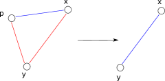
Figure 5: On the left a 2-structure $G$ with 3 vertices, on the right $G^{\odot}_{p}$.

Definition 2.3.

Switch Colors on 2-structures. Let $G=(X,E)$ be a 2-structure, $\mathcal{I}$ an involution of its colors and $s\in X$. We define $G^{\odot}_{s}$ as the 2-structure $(X^{\prime},E^{\prime})$, such that $X^{\prime}=X\setminus\{s\}$ and $\forall u,v\in X^{\prime}$, $E^{\prime}(u,v)=E^{\prime}(v,u)=\odot(E(s,u),E(s,v),E(u,v))$.

We mean here that we pick a vertex $s$, we call it the pivot, and for each couple of vertices $x,y$ different from $s$, we change the color of the edge $\{x,y\}$ following the colors of the edge $\{s,x\}$, $\{s,y\}$ and $\{x,y\}$. We now introduce the three following lemmas which ensure the correctness of the algorithm.

Lemma 2.7.

Let $G=(X,E)$ be a 2-structure with $c$ colors, $s\in X$, $G^{\prime}=G^{\odot}_{s}=(X^{\prime},E^{\prime})$ and $\mathcal{I}$ an involution of the colors.
Let $U\subset X$ such that $s\in U$, $U$ is an involution module of $G$. $X\setminus U$ is a module of $G^{\prime}$.

Proof.

Let $U\subseteq X$ be an involution module of $G$ such that $s\in U$ and $M=X\setminus U$. Let $A$ be the set of elements of $U$ that have the same outside neighborhood than $s$ and $B=U\setminus A$.

Then, for all elements $x\in A$ and $v\in M$, $E(x,v)=E(s,v)$. Therefore, when we apply the Switch_Colors, for any $x\in A$,we obtain $E^{\prime}(x,v)=\odot(E(s,v),E(s,x),E(x,v))=E(s,x)$. Thus, $x$ does not distinguish any element of $M$.

Now, for all elements $x\in B$ and $v\in M$, $E(x,v)=\mathcal{I}(E(s,v))$. Therefore, when we apply the Switch_Colors, for any $x\in B$,we obtain $E^{\prime}(x,v)=\odot(E(s,v),E(s,x),E(x,v))=\mathcal{I}(E(s,x))$. Thus, $x$ does not distinguish any element of $M$.

We can conclude that $M$ is a module of $G^{\prime}$. ∎

Lemma 2.8.

Let $G=(X,E)$ be a 2-structure with $c$ colors, $s\in X$, $G^{\prime}=G^{\odot}_{s}$ Let $U\subset X$ such that $s\in U$, $X\setminus U$ an involution module of $G$. $X\setminus U$ is a module of $G^{\prime}$.

Proof.

Let $U\subseteq X$ and $M=X\setminus U$ such that $s\in U$ and $M$ is an involution module. Then $s$ partitions $M$ into 2 parts $A$ and $B$ such that for any elements $a\in A$ and $b\in B$, $E(s,a)=\mathcal{I}(E(s,b))$.

Let $x$ be an element of $U$. Note that $x$ also splits $M$ into the same parts $A$ and $B$ (otherwise the elements of $M$ do not partition the graph the same way). When we apply the Switch_Colors on $G$, for all $a\in A$, $E^{\prime}(x,a)=\odot(E(s,a),E(s,x),E(x,a))$ and for all $b\in B$, $E^{\prime}(x,b)=\odot(E(s,b),E(s,x),E(x,b))=\odot(\mathcal{I}(E(s,a)),E(s,x),\mathcal{I}(E(x,a)))$. Hence, according to the definition of the Switch_Colors, $\odot(\mathcal{I}(E(s,a)),E(s,x),\mathcal{I}(E(x,a)))=\odot(E(s,a),E(s,x),E(x,a))$ and therefore $E^{\prime}(x,a)=E^{\prime}(x,b)$. $x$ does not distinguish any element of $M$ in $G^{\prime}$, we conclude that $M$ is a module of $G^{\prime}$. ∎

We now prove the converse of the two previous lemmas.

Lemma 2.9.

Let $G=(X,E)$ be a 2-structure with $c$ colors, $s\in X$ and $G^{\prime}=G^{\odot}_{s}$ and $\mathcal{I}$ an involution of the colors.
Let $U\subset X$ such that $s\in U$, $M=X\setminus U$ is a module of $G^{\prime}$. $U$ is an involution module of $G$ or $X\setminus U$ is an involution module of $G$.

Proof.

Assume towards contradiction that $M$ is a module of $G^{\prime}$ and neither $U$ nor $M$ are involution modules of $G$. Since the singletons are involution modules, note that $|M|>1$ and $|U|>1$.

If $U$ and $M$ are not involution modules then each of them induce a forbidden pattern in $G$.

Assume first that $M$ induces figure 4. Then we pick $w\in U$ and $u,v\in M$ such that $s,w,u,v$ induces figure 4. If $M$ is a module of $G^{\prime}=(V^{\prime},E^{\prime})$ then $\odot(E(s,w),E(s,u),E(w,u))=\odot(E(s,w),E(s,v),E(w,v))$. There are only two possible cases, either $E(s,u)=E(s,v)$ and $E(w,u)=\mathcal{I}(E(w,v))$ or $E(s,u)=\mathcal{I}(E(s,v))$ and $E(w,u)=E(w,v)$. Hence, by definition of Switch_Colors, in any case $\odot(E(s,w),E(s,u),E(w,u))\neq\odot(E(s,w),E(s,v),E(w,v))$, a contradiction.

Assume now $M$ induces figure 4. We can pick $v\in U$ and $a,b\in M$ such that $a,b,v$ induce figure 4 then. Now we distinguish the two possible cases, either $U$ is not an involution module because it induces figure 4 or because it induces figure 4.

In the first case, we can pick $u\in U$ and $a\in M$ such that $s,u,a$ induce figure 4. Now, since $M$ is a module of $G^{\prime}$, we have $E^{\prime}(v,a)=E^{\prime}(v,b)$ and $E^{\prime}(u,a)=E^{\prime}(u,b)$. Hence, $\odot(E(s,a),E(s,v),E(v,a))=\odot(E(s,b),E(s,v),E(v,b))$ and $E(v,b)\neq E(v,a),\mathcal{I}(E(v,a))$. By the Switch_Colors definition, this is true if and only if $E(s,a)=E(v,a)$ and $E(s,b)=E(v,b)$ or $E(s,a)=\mathcal{I}(E(v,a))$ and $E(s,b)=\mathcal{I}(E(v,b))$. Now, since $M$ is a module of $G^{\prime}$, $\odot(E(s,a),E(s,u),E(u,a))=\odot(E(s,b),E(s,u),E(u,b))$ and $E(s,a)\neq E(u,a),\mathcal{I}(E(u,a))$. By the Switch_Colors definition, this is true if and only if $E(s,a)=E(s,b)$ or $E(s,a)=\mathcal{I}(E(s,b))$, a contradiction.

In the latter case, we pick $b,c\in M$ and $u\in U$ such that $u,s,b,c$ induce figure 4. Now, either $E(s,b)=E(u,b)$ and $E(s,c)=\mathcal{I}(E(u,c))$ or $E(s,b)=\mathcal{I}(E(u,b)$ and $E(s,c)=E(u,c)$. If $E(s,b)=E(u,b)$ and $E(s,c)=\mathcal{I}(E(u,c))$ then $E^{\prime}(u,b)=\odot(E(s,b),E(s,u),E(u,b))=E(s,u)$ and $E^{\prime}(u,c)=\odot(E(s,c),E(s,u),E(u,c))=\mathcal{I}(E(s,u))$. Therefore $u$ distinguishes $c$ from $b$. $M$ is not a module of $G^{\prime}$, a contradiction.
If $E(s,b)=\mathcal{I}(E(u,b)$ and $E(s,c)=E(u,c)$ then $E^{\prime}(u,b)=\odot(E(s,b),E(s,u),E(u,b))=\mathcal{I}(E(s,u))$ and $E^{\prime}(u,c)=\odot(E(s,c),E(s,u),E(u,c))=(E(s,u)$. Therefore $u$ distinguishes $c$ from $b$. $M$ is not a module of $G^{\prime}$, a contradiction which concludes the proof. ∎

These three lemmas induce the following theorem.

Theorem 2.10.

Let $G=(X,E)$ be a 2-structure with $c$ colors, $s\in X$ and $G^{\prime}=G^{\odot}_{s}$.
Let $U\subset X$ such that $s\in U$. $M=X\setminus U$ is a module of $G^{\prime}$ $\iff$ $U$ is an involution module of $G$ or $X\setminus U$ is an involution module of $G$.

This theorem is of particular importance because it guarantees that the tree-representation of the family of involution modules of any 2-structure $G=(X,E)$ is almost the same than the tree-representation of the family of modules of the 2-structure $G^{\odot}_{s}$, for any $s\in X$. This is what we state below.

Proposition 2.11.

Let $G=(X,E)$ be a 2-structure and $s$ be an element of $X$. The involution modular decomposition tree $\mathcal{T}$ of $G$ and the modular decomposition tree $\mathcal{T}_{G^{\odot}_{s}}$ of $G^{\odot}_{s}$ have the following properties:

• The two trees have the same nodes except that the leaf with label $s$ is missing in $\mathcal{T}_{G^{\odot}_{s}}$ but present in $\mathcal{T}$.

• The node of $\mathcal{T}$ that is adjacent to the leaf $s$ corresponds to the root of $\mathcal{T}_{G^{\odot}_{s}}$ (while $\mathcal{T}$ is unrooted).

• The prime and complete nodes are the same in both trees.

Proof.

This is a direct consequence of theorem 2.10. Each strong module of $\mathcal{T}_{G^{\odot}_{s}}$ is a strong involution module or the complement of a strong involution module of $G$ and the converse holds. Therefore, for any complete node $N$ of $\mathcal{T}_{G^{\odot}_{s}}$, the union of any subset of the neighbors of $N$ is a module of $G^{\odot}_{s}$ and thus it is an involution module or the complement of an involution module of $G$. The same reasoning applies for the prime nodes. For each involution module $U$ and its complement $X\setminus U$, the part which contains $s$ is dropped and the other part is included in the family of modules of $G^{\odot}_{s}$. Thus, the neighbor of node $s$ in $\mathcal{T}_{G}$ is the root of $\mathcal{T}_{G^{\odot}_{s}}$. ∎

For any 2-structure, the tree computed by our algorithm is exactly an undirected version of the tree-representation of the family of involution modules of the 2-structure.

We now show how to determine the direction of the edges of the tree. Let us first recall a theorem from [6].

Theorem 2.12.

[6]. The tree-representation $\mathcal{T}$ of any weakly partitive crossing family has either one sink or only one double-arc $uv$ such that $\mathcal{T}\setminus uv$ has two sinks $u$ and $v$.

We now proceed bottom-up in order to direct the edges. The algorithm is as follow, first we direct the edges until we find a vertex which has only in arcs. By theorem 2.12, either this vertex is the sink of the tree or it shares a double arc with one of its neighbors. We then consider the edges that are adjacent to the sink vertex in order to determine whether there is a double arc or not.

Definition 2.4.

Edge Direction Algorithm.

Phase 1

We begin by the leaves - which are always involution modules so that they all have an out arc. Then for each leaf $l$ we can check whether $X\setminus\{l\}$ is an involution module. If we find a leaf whose complement is also an involution module then we are done: the out arc of the leaf is the double-arc and we direct the edges to the leaf.

Phase 2

Then we perform bottom-up by considering all the nodes that have at most one edge undirected. If a node has one out arc then we direct the other edges to the node. Now, consider a node $N$ with $k+1$ neighbors with only one undirected edge and $k$ in arcs. For each neighbor $V$, we pick a vertex which is a leaf of the subtree rooted at $V$. Call the set of chosen vertices $S$ and let $W$ be the neighbor whose edge to $N$ is undirected. Then, we check that $S$ is an involution module for the 2-structure $G_{[S\cup V(W)]}$ where $V(W)$ is the set of leaves whose paths to $N$ traverse $W$. If this set is an involution module then the union of the sets of the leaves of the subtrees rooted at the processed neighbors of $V$ is an involution module (since each set is an involution module and because of the union stability). We can therefore direct the edge from $V$ to $W$. Otherwise we direct the edge from $W$ to $V$. Phase 2 terminates when we find a sink vertex $u$.

Phase 3

Now, we only need to test whether this sink vertex has a double arc with one of its neighbor. Note that for each neighbor $N$ the set of leaves of the subtree rooted at $N$ is an involution module of $G$. Let $k$ be the number of neighbors of $u$ and $N_{k}$ be the set of leaves of the subtree rooted at the $k^{th}$ neighbor of $u$. For each of the $k-1$ remaining neighbors, we pick a vertex. Let call $S$ the set of these vertices. We first check whether this set is an involution module of the 2-structure $G_{[N_{1}\cup S]}$. If it is, then we are done. Otherwise we drop the vertex of the second neighbor and we pick a vertex of the first neighbor and we check whether this set is an involution module of the 2-structure $G_{[N_{2}\cup S]}$ and so on until we find a set which is an involution module (and thus a double arc) or not (and thus $N$ is the unique sink of the tree).

We can now state the following theorem.

Theorem 2.13.

The Edge Direction Algorithm computes the direction of the edges of the involution modular tree-decomposition of any 2-structure $G=(X,E)$ with an $\mathcal{O}(|X|^{2})$ time complexity.

Proof.

The correctness of the algorithm follows from theorem 2.12, lemma 2.2 and the definition.

We now show that the time complexity of the algorithm is $\mathcal{O}(|X|^{2})$. Notice first that one can greedily check whether a set of size $k$ is an involution module of a 2-structure $G=(X^{\prime},E^{\prime})$ in $C.k.(|X^{\prime}|-k)$ operations for some constant $C$ by checking for each vertex of the set if the partition of the rest of the 2-structure coincides with the partition of the already processed vertices and by reccording an adjacency matrix of the colors of the 2-structure.

The cost of phase 1 is thus $\mathcal{O}(|X|^{2})$ since there is exactly $|X|$ leaves.

Then during phase 2, for each node $N$ the cost is at most $C.k.|X|$ where $k$ is the number of neighbors of $N$. By taking the sum over all the nodes of the tree we obtain an $\mathcal{O}(|X|^{2})$ for the complexity of phase 2.

Let us now consider the third phase. Assume that $U$ has $k$ neighbors. For the $i^{th}$ neighbor we have to check whether the set $S$ is an involution module of the 2-structure $G_{[S\cup N_{i}]}$. The cost is at most $C.k.|N_{i}|$. Note that the sum of all the $N_{i}$ is exactly $|X|$. Therefore by taking the sum over all the neighbors of $U$ we obtain an overall cost of $C.k.|X|$. Since $k\leq|X|$, the complexity of phase 3 is $\mathcal{O}(|X|^{2})$.

Therefore, the complexity of the algorithm is $\mathcal{O}(|X|^{2})$.

∎

Theorem 2.13 and proposition2.11 allow us to conclude this section with the following theorem.

Theorem 2.14.

There exists an $\mathcal{O}(n^{2})$ algorithm which computes the tree representation of the family of the involution modules of any 2-structure.

Proof.

The algorithm consists in picking a vertex $s$ and applying the operator Switch Colors to the 2-structure. This can be done in $\mathcal{O}(n^{2})$ by considering each edge once and applying the rules described above. Then we apply the $\mathcal{O}(n^{2})$ modular decomposition algorithm of [13] and we obtain the tree. We then apply the Edge Direction Algorithm in order to compute the direction of the edges of the tree.

Theorems 2.10 and 2.13 and proposition 2.11 ensure the correctness of the algorithm. ∎

Before moving to the next section, we recall the definition of the Seidel Switch and remark that our Switch Colors operator generalizes the Seidel Switch to 2-structures.

Definition 2.5.

Seidel Switch. Let $G=(X,E)$ be a graph and $v\in E$. The Seidel Switch applied at $v$ on $G$ consists in complementing the edges and non-edges of neighbors and non-neighbors of $v$ before removing $v$. The resulting graph is

$G^{\prime}=(X\setminus v,E^{\prime})$ where $E^{\prime}=E\bigtriangleup\{xy|vx\in E,vy\notin E\}$.

Remark.

Seidel Switch. The Switch Colors operator applied to undirected graphs coincides with the Seidel Switch defined in [23]. One can see the Switch Colors operator as a generalization of the Seidel Switch to 2-structures.

3 Switch Cographs

We now focus on undirected graphs - which are symmetric 2-structures with two colors - and we use our new decomposition tool in order to state structural properties and design algorithms. Let us first remark that there is only one involution without fix point for the case of graphs so that we do not have to quantify on the involution throughout this section.

The modular decomposition led to study the classes of graphs which have a particular tree-decomposition. The best-known class is the class of cographs whose tree-decompositions have only complete nodes (they are called completely decomposable with respect to modular decomposition). [9] that the class of cographs is exactly the class of $P_{4}$-free graphs (i.e the class with no induce path with four vertices). [3] showed that the class of ($P_{5}$, Gem)-free graphs is a good generalization of the class of cographs since they have Clique-width at most 5 and thus some classical graph problems (the stable set problem for example) are polynomially tractable. Nevertheless this class only provides a Clique-width decomposition expression and no tree-decomposition (unlike cographs). Tree-decomposition is a powerful tool that can led to solve even more problems than a Clique-width decomposition expression (which helps to solve problems expressible by monadic second order logic without edge set quantification [10]) for particular classes of graphs.

Since the concept of involution module generalizes strictly the concept of module, an obvious and well-founded problem to address consists in characterizing and studying the class of graphs completely decomposable with respect to involution modular decomposition. This class of graphs generalizes strictly the class of cographs.

We show that this class is the class of (Gem, Co-gem, Bull, $C_{5}$)-free graphs (refer to figure 6), introduced by [19] as the class of switching-perfect graphs - the class of graphs which leads to a perfect graph after a Seidel Switch - and studied by [11] who gave a linear algorithm for the switch cograph isomorphism problem. We use the involution modular decomposition to tackle well-known graph problems.

First, we begin by highlighting structural properties of particular importance.

Figure 6: From left to right and top to bottom, the Gem, Co-gem, Bull and $C_{5}$ graphs

Definition 3.1.

(Twin,Antitwin)-extension. A (twin,Antitwin)-extension of a graph $G$ is a graph $G^{\prime}$ which consists of $G$ and a new vertex $v$ which is either a twin (i.e it has the same neighborhood than another vertex) or an antitwin (i.e the complement of its neighborhood coincides with the neighborhood of another vertex) of at least one vertex of $G$.

3.1 Structural Properties

Theorem 3.1.

Let $G$ be an undirect graph. The following definitions are equivalent:

1. $G$ is a switch cograph;

2. The umodular and involution modular decomposition trees of $G$ do not contain any prime node;

3. Let $p\in V$, and $G^{\prime}$ the graph corresponding to $G$ after a Seidel Switch on $p$. $G^{\prime}$ is a cograph;

4. $G$ has no induced Gem, Co-Gem, $C_{5}$ nor Bull subgraphs;

5. The class of switch cographs is the class of graphs which can be obtained from a single vertex by a sequence of (twin,antitwin)-extensions.

Proof.

[11] showed that $1\iff 3\iff 4$.
Theorem 2.10 implies that $1\iff 2$ because the labels of the two trees are the same. ∎

Lemma 3.2.

Binary Decomposition Tree. For any Switch Cograph, there exists a decomposition tree with maximum degree equal to 3.

Proof.

Let $G=(V,E)$ be a switch cograph, $p\in V$, and $G^{\prime}$ the graph corresponding to $G$ after a Seidel Switch on $p$. Since the decomposition tree of $G$ coincides with the decomposition tree of $G^{\prime}$, $G$ has maximum degree equal to 3 if and only if $G^{\prime}$ has maximum degree equal to 3. There exists a lemma from [1], saying that any cograph has a tree representation with degree at most 3 which concludes the proof. ∎

Notice that this tree is not canonical. Throughout this section, for any graph $G=(V,E)$ we denote by $n$ the cardinality of set $V$ and by $m$ the cardinality of set $E$.

Remark.

The class of switch cographs is closed under complement because the set of forbidden subgraphs is closed under complement Besides, the decomposition tree of the complement graph of any switch cograph can be computed in $\mathcal{O}(n+m)$ by computing the involution modular decomposition tree and changing each clique node into a bipartite node and vice versa.

Lemma 3.3.

Every switch cograph is a perfect graph.

Proof.

First notice that there is no hole nor anti-hole of length five since the switch cographs are $C_{5}$-free. Then, if there is an odd hole (resp. an odd anti-hole) of lenght greater than 7, it contains an induced Co-gem (resp. an induced Gem) which is a forbidden subgraph. Thus, switch cographs are bull-free berge graphs and so, perfect by [8]. ∎

3.2 Algorithmic paradigm

Throughout this section, we propose algorithms which traverse the decomposition tree of the switch cographs in a bottom-up fashion in the same way as it is done in [1] for the cographs. Namely, for any switch cograph $G$ an edge of its binary involution modular decomposition tree is picked and an artificial node is created on it. Then the tree is rooted at this node. A node is processed when its two children have already been processed.

Let us now introduce some notations, for any switch cograph $G$ and for any node $N$ of its binary involution modular decomposition tree and its two children $A$ and $B$, we note $G_{[N]}$ the subgraph of $G$ induced by the leaves of the subtree rooted at $N$.

By [11], the nodes of the binary involution modular decomposition tree are of two kinds. We distinguish the clique node (figure 8) and the bipartite node (figure 8). In any case, the graph $G_{[N]}$ can be split into two parts such that there exists $A_{1},A_{2}$ bipartition of $A$; $B_{1},B_{2}$ bipartition of $B$; and $C_{1},C_{2}$ bipartition of $C$ (where $C$ is the parent of $N$ in the rooted tree) such that, for the clique node, there are all the edges between the elements of $A_{1}$ and $B_{1}\cup C_{1}$ and no edge to elements of $B_{2}\cup C_{2}$, there are all the edges between elements of $A_{2}$ and elements of $B_{2}\cup C_{2}$ and no edge to elements of $B_{1}\cup C_{1}$, there are all the edges between elements of $B_{1}$ and elements of $A_{1}\cup C_{1}$ and no edge to elements of $A_{2}\cup C_{2}$ and there are all the edges between elements of $B_{2}$ and elements of $A_{2}\cup C_{2}$ and no edge to elements of $A_{1}\cup C_{1}$. The bipartite node is the complement of the clique node, i.e builds the clique node and complements the edges and non-edges created.

We note $N=(N_{1},N_{2})$ to refer to the node $N$ and its two parts.

This lead to the following crucial lemma.

Lemma 3.4.

Let $G=(V,E)$ be a switch cograph and $N=(N_{1},N_{2})$ a node of its involution modular binary decomposition tree and $A=(A_{1},A_{2})$ and $B=(B_{1},B_{2})$ its two children. Then, either $N_{1}=A_{1}\cup B_{1}$ and $N_{2}=A_{2}\cup B_{2}$; or $N_{1}=A_{1}\cup B_{2}$ and $N_{2}=A_{2}\cup B_{1}$; or $N_{1}=A_{2}\cup B_{2}$ and $N_{2}=A_{1}\cup B_{1}$; or $N_{1}=A_{2}\cup B_{1}$ and $N_{2}=A_{1}\cup B_{2}$.

Proof.

Assume towards contradiction that there exists a clique node $N=(N_{1},N_{2})$ with two children $A=(A_{1},A_{2})$ and $B=(B_{1},B_{2})$ such that the bipartitions of $A$ and $B$ is not respected at $N$. Let $C=(C_{1},C_{2})$ be the third neighbor of $N$.

Now, let $A_{1}^{\prime}=N_{1}\cap A$, $B_{1}^{\prime}=N_{1}\cap B$, $A_{2}^{\prime}=N_{2}\cap A$ and $B_{2}^{\prime}=N_{2}\cap B$. W.l.o.g we can assume that $A_{1}\cap N_{1}\neq\emptyset$ and $A_{1}\cap N_{2}\neq\emptyset$. Consider now the node $A=(A_{1},A_{2})$, and its two children $D$ and $E$ and its third neighbor which is the rest of the graph, namely $G_{[B\cup C]}$.

Then there are all the edges between the elements of $C_{1}\cup B_{1}^{\prime}$ and the elements of $A_{1}^{\prime}$. So if $\exists a\in A_{1}^{\prime}\setminus A_{1}$, it implies that $a$ is connected to every element of $C_{1}\cup B_{1}^{\prime}$ and so $a\in A_{1}$, a contradiction. If $\exists a\in A_{1}\setminus A_{1}^{\prime}$, it implies that $a$ has no edges with $C_{1}\cup B_{1}^{\prime}$ and so $a\notin A_{1}$, a contradiction. Thus, $A_{1}=A_{1}^{\prime}$, a contradiction.

The same reasoning applies to the bipartite node case. ∎

Then for any node $N=(N_{1},N_{2})$, we refer to its two children $A$ and $B$ as $A=(A_{1},A_{2})$ and $B=(B_{1},B_{2})$ such that $N_{1}=A_{1}\cup B_{1}$ and $N_{2}=A_{2}\cup B_{2}$. Thus, for a clique node $A_{1}$ and $B_{1}$ are connected in a clique fashion and $A_{2}$ and $B_{2}$ as well and for a bipartite node $A_{1}$ and $B_{1}$ are not adjacent and $A_{2}$ and $B_{2}$ either (see figures 8 and 8).

Lemma 3.5.

Let $G=(V,E)$ be a switch cograph and $N=(N_{1},N_{2})$ a node of its involution modular binary decomposition tree (IMDT). $G_{[N_{1}]}$ and $G_{[N_{2}]}$ are cographs.

Proof.

First, for all $i,j\in\{1,2\}$, $i\neq j$, $G_{[A_{i}]}$ (resp. $G_{[B_{i}]}$) is a cograph (proof: if $A_{i}$ or $A_{j}$ (resp. $B_{i}$ or $B_{j}$) contains a $P_{4}$ and $B_{i}\cup B_{j}$ (resp. $A_{i}\cup A_{j}$) is not empty there is an induced Gem or Co-gem). Then, since $A_{i}$ and $B_{i}$ are both cographs and are either connected in a clique fashion or not adjacent at all, by lemma 3.4 $N_{i}$ is a cograph. ∎

Since the IMDT and the umodular decomposition tree coincide for graphs, we recall the following lemma.

Lemma 3.6.

[5]. The binary IMDT of a switch cograph can be computed in $\mathcal{O}(n+m)$.

Remark.

Notice that the IMDT provides an efficient tool for switch cographs recognition. To test whether a graph is a switch cograph, compute its IMDT and check that each node of the tree is a complete node. These operations can be done in $\mathcal{O}(n+m)$ thanks to lemma 3.6.

Before we start, we state the following lemma that will help for the complexity analysis of the following algorithms.

Lemma 3.7.

Let $\mathcal{T}$ a rooted binary tree of size $\mathcal{O}(n)$ and $\mathcal{A}$ be an algorithm which proceeds bottom-up on $\mathcal{T}$.

Let $N$ be a node of $\mathcal{T}$ whose subtree contains $n_{N}$ nodes and $A$ and $B$ be its two children whose subtrees respectively contains $n_{A}$ and $n_{B}$ nodes. If the running time of the algorithm at node $N$ assuming that its two children have already been computed is less than $n_{A}^{C/2}*n_{B}^{C/2}$, then the overall complexity of the algorithm is $\mathcal{O}(n^{C})$, for some constant $C\geq 1$.

Proof.

First, notice that the complexity of the algorithm is some constant $c$ for the leaves of the tree. We show by induction that the complexity of the algorithm at a node $N$ is less than $c.n_{N}^{C}$. We assume that this holds for any node at a distance of at most $k$ from a leaf. We show that this is true for a node at a distance $k+1$. Let $N$ be such a node and $A$ and $B$ be its two children.

By induction, the running time of the algorithm to process $A$ and $B$ is less than $c.(n_{A}^{C}+n_{B}^{C})$.Therefore, the overall time computation at node $N$ is less than $c.(n_{A}^{C}+n_{B}^{C}+(n_{A}^{C/2}*n_{B}^{C/2}))\leq c.(n_{A}+n_{B})^{C}=n^{C}$.

We conclude that the algorithm takes $\mathcal{O}(n^{C})$ computation time. ∎

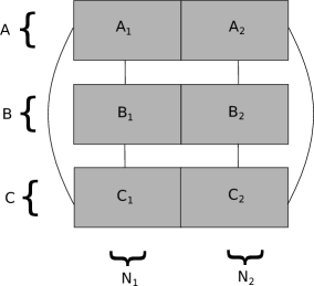
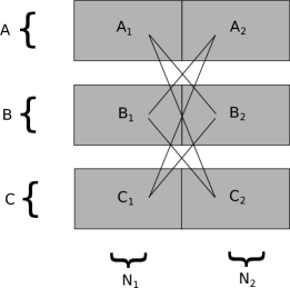
Figure 7: Clique Node. A node $N=(N_{1},N_{2})$ of a binary IMDT of a switch cograph such that $A=(A_{1},A_{2})$, $B=(B_{1},B_{2})$ and $C=(C_{1},C_{2})$ are its three neighbors and $A_{1},B_{1},C_{1}$ are connected in a clique fashion and $A_{2},B_{2},C_{2}$ as well.

Figure 8: Bipartite Node. A node $N=(N_{1},N_{2})$ of a binary IMDT of a switch cograph such that $A=(A_{1},A_{2})$, $B=(B_{1},B_{2})$ and $C=(C_{1},C_{2})$ are its three neighbors and they are connected in a bipartite fashion.

3.3 Maximum Clique Problem

We now tackle the maximum clique problem, namely:

Definition 3.2.

Maximum Clique Problem.
Instance: A graph $G=(V,E)$.
Problem: Find the size of a maximum complete subgraph of $G$.

Let $G$ be a switch cograph, $N=(N_{1},N_{2})$ be a node of the tree and $A=(A_{1},A_{2}),B=(B_{1},B_{2})$ be its two children.

Lemma 3.8.

Maximum Clique on switch cographs. Let $G$ be a switch cograph, $N$ be a node of its involution modular binary IMDT and $A=(A_{1},A_{2})$ and $B=(B_{1},B_{2})$ be its two children.

If $N$ is a clique node

, then the maximum clique of $G$ is the maximum clique among the maximum clique of $N_{1}$ , the maximum clique of $N_{2}$ , the maximum clique of $A$ and the maximum clique of $B$.

If $N$ is a bipartite node

, then the maximum clique of G is the maximum clique among the maximum clique of $G_{[A_{1}\cup B_{2}]}$ , the maximum clique of $G_{[A_{2}\cup B_{1}]}$ , the maximum clique of $A$ and the maximum clique of $B$.

Proof.

We first give the proof for the clique case. The maximum clique of $G_{[N]}$ cannot contain simultaneously elements of $A_{1}$ and $B_{2}$ nor simultaneously elements of $B_{1}$ and $C_{2}$ (since there is no edge between these elements). Therefore, if the maximum clique contains elements of $A_{i}$ (resp $B_{j}$) then it can contain elements of $B_{i}$ (resp $A_{j}$) and in this case no element of $A_{3-i}$ (resp $B_{3-j}$) or the converse ($i\in\{1,2\}$).

Let us now consider the bipartite case. The maximum clique of $G_{[N]}$ cannot contain simultaneously elements of $A_{1}$ and $B_{1}$ nor simultaneously elements of $A_{2}$ and $B_{2}$ (since there is no edge between these elements). Therefore, if the maximum clique contains elements of $A_{i}$ (resp $B_{j}$) then it can contain elements of $B_{j}$ (resp $A_{i}$) and in this case no element of $A_{3-i}$ (resp $B_{3-j}$) or the converse ($i\in\{1,2\}$). ∎

We now show that we are able to compute these values for each node of the binary IMDT (assuming we already computed the corresponding values for its children).

Theorem 3.9.

The maximum clique problem can be solved with a linear time complexity when restricted to switch cographs.

Proof.

Going from the leaves of the tree to its arbitrary-chosen root, for each node $N$ with $A=(A_{1},A_{2})$ and $B=(B_{1},B_{2})$ its two children. We distinguish the two cases:

Clique Case:

If $N=(N_{1},N_{2})$ is a clique node such that $A_{1}$,$B_{1}$ and $A_{2},B_{2}$ are completely joined. We first compute the size of the largest clique of $G_{[N_{1}]}$ (resp. $G_{[N_{2}]}$), which is, by lemma 3.8 sum of the size of the largest clique of $G_{[A_{1}]}$ (resp. $A_{2}$) and the size of the largest clique of $G_{[B_{1}]}$ (resp. $G_{[B_{2}]}$). This operation can be done in $\mathcal{O}(1)$ by lemma 3.4. We can now compute the maximum clique of $G_{[N]}$ which is the maximum among the maximum clique of $G_{[N_{1}]}$, the maximum clique of $G_{[N_{2}]}$, the maximum clique of $G_{[A]}$ and the maximum clique of $G_{[B]}$. This operation can be done in $\mathcal{O}(1)$ provided we already computed the largest clique of its children and by lemma 3.4.

Bipartite Case:

If $N=(N_{1},N_{2})$ is a bipartite node such that $A_{1}$,$B_{2}$ and $A_{2}$,$B_{1}$ are completely joined. We first compute the size of the largest clique on $G_{[N_{1}]}$ (resp. $G_{[N_{2}]}$), which is, by lemma 3.8 the maximum of the size of the largest clique of $G_{[A_{1}]}$ (resp. $A_{2}$) and the size of the largest clique of $G_{[B_{1}]}$ (resp. $G_{[B_{2}]}$). This operation can be done in $\mathcal{O}(1)$ by lemma 3.4. We can now compute the maximum clique of $G_{[N]}$ which is the maximum among the maximum clique of $G_{[N_{1}]}$, the maximum clique of $G_{[N_{2}]}$, the maximum clique of $G_{[A]}$ and the maximum clique of $G_{[B]}$. This operation can be done in $\mathcal{O}(1)$ provided we already computed the largest clique of its children and by lemma 3.4.

There are $\mathcal{O}(n)$ nodes on the tree-decomposition, the tree-decomposition can be computed in $\mathcal{O}(n+m)$, this leads to an $\mathcal{O}(n+m)$ algorithm to compute the maximum clique of a switch cograph. ∎

Corollary.

The maximum independant set problem can be solved with a linear time complexity when restricted to switch cographs.

Proof.

The same reasoning applies when computing an independant set. ∎

Corollary.

The chromatic number problem can be solved with a linear-time complexity when restricted to switch cographs.

Proof.

The class of switch cographs is included in the class of perfect graphs. ∎

Corollary.

The Clique Cover and Independant Set Cover problems can be solved with a linear time complexity when restricted to switch cographs.

Proof.

The class of switch cographs is closed under complement and the chromatic number of a switch cograph can be computed in linear time. ∎

3.4 Vertex Cover Problem

Let us now address the minimum vertex cover problem on switch cographs.

Definition 3.3.

Minimum Vertex Cover Problem.
Instance: A graph $G=(V,E)$.
Problem: Find a set of vertices $X$ such that $\forall\{x,y\}\in E$, $x\in X$ or $y\in X$ whose size is minimum.

We first introduce the two following lemmas.

Lemma 3.10.

Vertex Cover Problem on complete bipartite subgraphs. Let $G=(A,B)$ be a complete bipartite subgraph of a graph $H=(V,E)$. Let $S$ be a solution to the Vertex Cover Problem for $H$. Then, either $A\subseteq S$ or $B\subseteq S$.

Proof.

Suppose that neither $A$ or $B$ is included in $S$. Then there exists $a\in A$, $b\in B$ such that $a,b\notin S$. But because $G=(A,B)$ is a complete bipartite subgraph, it means that the edge $(a,b)\in E$ is not covered by $S$, a contradiction which concludes the proof. ∎

Lemma 3.11.

Vertex Cover Problem for Switch Cographs. Let $G$ be a switch cograph, $N=(N_{1},N_{2})$ a node of its binary IMDT and $A=(A_{1},A_{2})$ and $B=(B_{1},B_{2})$ be its two children.The minimal Vertex Cover for $G_{[N]}$ is the minimal solution among:

If $N$ is a clique node

:

(1)

$S_{1}=A_{1}\cup A_{2}\cup S_{B}$;

(2)

$S_{2}=B_{1}\cup B_{2}\cup S_{A}$;

(3)

$S_{3}=A_{1}\cup B_{2}\cup S_{B_{1}}\cup S_{A_{2}}$;

(4)

$S_{4}=A_{2}\cup B_{1}\cup S_{B_{2}}\cup S_{A_{1}}$;

If $N$ is a bipartite node

:

(1)

$S_{5}=A_{1}\cup A_{2}\cup S_{B}$;

(2)

$S_{6}=B_{1}\cup B_{2}\cup S_{A}$;

(3)

$S_{7}=A_{1}\cup B_{1}\cup S_{B_{2}}\cup S_{A_{2}}$;

(4)

$S_{8}=A_{2}\cup B_{2}\cup S_{B_{1}}\cup S_{A_{1}}$;

where $S_{A}$, $S_{B}$, $S_{A_{1}}$, $S_{A_{2}}$, $S_{B_{1}}$ and $S_{B_{2}}$ are respectively vertex cover solutions to $G_{[A]}$, $G_{[B]}$, $G_{[A_{1}]}$, $G_{[A_{2}]}$, $G_{[B_{1}]}$ and $G_{[B_{2}]}$.

Proof.

First, notice that cases (1) and (2) are symmetric (and (3) and (4) as well) regardless of whether $N$ is a clique or a bipartite node.

If $N$ is a clique node

: By lemma 3.10, either $A_{1}$ or $B_{1}$ (resp $A_{2}$ or $B_{2}$) is included in $S$. We consider the two possible cases (up to symmetry), $A_{1}\cup A_{2}\in S$ or $A_{1}\cup B_{2}\in S$.

In the first case, it is guaranted that all the edges between elements of $A$ and all the edges between $A$ and $B$ are covered, therefore we just need to cover the edges of $B$ and we use the solution for $G_{[B]}$ to cover them. This proves the cases (1) (and (2) likewise).

In the second case, it is guaranted that all the edges between $A_{1}$ (resp $B_{2}$) and $B_{1}\cup A_{2}$ are covered. We just need to cover the edges between elements of $B_{1}$ and the edges between elements of $A_{2}$. This proves cases (3) (and (4) likewise).

Since these cases are the only possible cases, this completes the clique node case proof.

If $N$ is a bipartite node

: By lemma 3.10, either $A_{1}$ or $B_{1}$ (resp $A_{2}$ or $B_{2}$) is included in $S$. We consider the two possible cases (up to symmetry), $A_{1}\cup A_{2}\in S$ or $A_{1}\cup B_{2}\in S$.

In the first case, it is guaranted that all the edges between elements of $A$ and all the edges between $A$ and $B$ are covered, therefore we just need to cover the edges of $B$ and we use the solution for $G_{[B]}$ to cover them. This proves the cases (1) (and (2) likewise).

In the second case, it is guaranted that all the edges between $A_{1}$ (resp. $B_{1}$) and $B_{2}\cup A_{2}$ (resp. $A_{2}\cup B_{2}$) are covered. We just need to cover the edges between elements of $B_{2}$ and the edges between elements of $A_{2}$. this proves the cases (3) and ((4) likewise).

Since these cases are the only possible cases, this completes the bipartite node case proof.

∎

Theorem 3.12.

The Vertex Cover Problem can be solved with a linear time complexity when restricted to switch cographs.

Proof.

We propose a bottom-up algorithm, from the leaves of the tree to its root. We claim that we are able to compute for each node $N=(N_{1},N_{2})$ of the tree, an optimal solution to Vertex Cover for $N$, $N_{1}$, and $N_{2}$ in constant time provided the solutions to the vertex cover problem on the children of $N$.

This is obviously true for the leaves since there is only one node. Assume that this holds for any node at a distance of at most $k$ from the root and we show that this holds for a node at a distance $k-1$.

Let $N=(N_{1},N_{2})$ be such a node and $A=(A_{1},A_{2})$ and $B=(B_{1},B_{2})$ be its two children.

Clique Node:

If $N$ is a clique node. We first show that we are able to compute $S_{N_{1}}$ (resp $S_{N_{2}}$) a solution to vertex cover to the subgraph $G_{[N_{1}]}$ (resp $G_{[N_{2}]}$). By lemma 3.10, either $A_{1}$ or $B_{1}$ is included in $S_{N_{1}}$.

If all the elements of $A_{1}$ are included then we just need to cover the edges of $G_{[B_{1}]}$ so we add $A_{1}$ to the solution to vertex cover for $G_{[B_{1}]}$. By induction hypothesis and lemma 3.4 we already computed this solution. If all the elements of $B_{1}$ are included we just need to cover the edges of $G_{[A_{1}]}$ so we add $B_{1}$ to the solution to vertex cover for $G_{[A_{1}]}$. By induction hypothesis and lemma 3.4 we also computed this solution.

These cases are the two possible cases, so the solution to vertex cover for $G_{[N_{1}]}$ is the smallest among these two cases. We can do the same operation to compute an optimal solution for $G_{[N_{2}]}$.

Bipartite Node:

If $N$ is a bipartite node. We first show that we are able to compute $S_{N_{1}}$ (resp $S_{N_{2}}$) a solution to vertex cover to the subgraph $N_{1}$ (resp $N_{2}$). Since there is no edge between $G_{[A_{i}]}$ and $G_{[B_{i}]}$, the solution for $G_{[N_{i}]}$ is $S_{A_{i}}\cup S_{B_{i}}$ where $S_{A_{i}}$ and $S_{B_{i}}$ are the solution for $G_{[A_{i}]}$ and $G_{[B_{i}]}$. By induction hypothesis and lemma 3.4, these solutions are already computed.

We now show that we are able to compute a solution for $G_{[N]}$. By lemma 3.11 there are only 4 different cases and by induction hypothesis and lemma 3.4 we have already computed the solutions for $G_{[A_{1}]},G_{[A_{2}]},G_{[B_{1}]},G_{[B_{2}]},G_{[A]}$ and $G_{[B]}$. Thus we can choose the smallest among the four cases we described above to be the solution for $G_{[N]}$.

We now prove the complexity and correctness of the algorithm.

Correctness

: By lemma 3.11, 3.10, 3.4.

Complexity

: At each node, we compute the minimum over 4 values. The tree has $\mathcal{O}(n)$ nodes, the tree-decomposition is computed in $\mathcal{O}(n+m)$ the complexity of the algorithm is therefore $\mathcal{O}(n+m)$.

∎

3.5 Maximum Cut Problem

Whereas the clique-width of switch cographs is bounded (see section 3.7), the complexity of the maximum cut problem remained open. This problem is not expressible in monadic second order logic ([15]) and therefore is not caught by the famous theorem of Courcelle et al. [10]. This shows that our decomposition tool provides us with even more algorithmic properties than the clique-width decomposition for the class of switch cographs.

Definition 3.4.

Maximum Cut Problem.
Instance: A graph $G=(V,E)$.
Problem: Find two sets of vertices $A$ and $B$ such that $A\cap B=\emptyset$ and the set $\{\{x,y\}$ $|$ $\{x,y\}\in E$, $x\in A$ and $y\in B\}$ has maximum size.

In order to compute the Maximum Cut of a switch cograph we will use a dynamic programming approach. We first prove two lemmas of particular importance.

Lemma 3.13.

Maximum Cut on Switch Cographs. Let $G=(V,E)$ be a switch cograph and $N=(N_{1},N_{2})$ a node of its IMDT and $A=(A_{1},A_{2})$ and $B=(B_{1},B_{2})$ its two childen. Let us define $C_{N}$ be a $|V|\times|V|$ array such that $C_{N}[i,j]$ equals the size of a maximum cut $(X,Y)$ such that $|X\cap N_{1}|=i$ and $|X\cap N_{2}|=j$. Then

If $N$ is a clique node

:
$C_{N}[i,j]=\max\limits_{\scriptsize\begin{array}[]{c}k+l=i\\ q+r=j\end{array}}C_{A}[l,q]+C_{B}[k,r]+l(|B_{1}|-k)+k(|A_{1}|-l)+q(|B_{2}|-r)+r(|A_{2}|-q)$

If $N$ is a bipartite node

:
$C_{N}[i,j]=\max\limits_{\scriptsize\begin{array}[]{c}k+l=i\\ q+r=j\end{array}}C_{A}[l,q]+C_{B}[k,r]+q(|B_{1}|-k)+k(|A_{2}|-q)+l(|B_{2}|-r)+r(|A_{1}|-l)$

Proof.

We distinguish the two sorts of nodes.

If $N$ is a clique node

Let $S=(X,Y)$ be a maximum cut of value $v$ such that $|X\cap N_{1}|=i$, $|X\cap N_{2}|=j$, $|X\cap A_{1}|=l$, $|X\cap A_{2}|=q$, $|X\cap B_{1}|=k$ and $|X\cap B_{2}|=r$.

Assume towards contradiction that $v>C_{N}[i,j]=C_{A}[l,q]+C_{B}[k,r]+l(|B_{1}|-k)+k(|A_{1}|-l)+q(|B_{2}|-r)+r(|A_{2}|-q)$.

Since there are $l$ elements from $A_{1}$ in $X$ and $k$ elements from $B_{1}$ in $X$, there are $l(|B_{1}|-k)+k(|A_{1}|-l)$ edges crossing the cut in $G_{1}$. The same reasoning applies to $G_{2}$.

Now, let $v_{A}$ (resp. $v_{B}$) be the value of the cut $S$ restricted to the edges of $G_{[A]}$ (resp. $G_{[B]}$). Since $v$ is strictly greater than $C_{N}[i,j]$ it means that $v_{A}+v_{B}>C_{A}[l,q]+C_{B}[k,r]$. By induction hypothesis and lemma 3.4, we have both $C_{A}[l,q]\geq v_{A}$ and $C_{B}[k,r]\geq v_{B}$, a contradiction which concludes the proof.

If $N$ is a bipartite node

Let $S=(X,Y)$ be a maximum cut of value $v$ such that $|X\cap N_{1}|=i$, $|X\cap N_{2}|=j$, $|X\cap A_{1}|=l$, $|X\cap A_{2}|=q$, $|X\cap B_{1}|=k$ and $|X\cap B_{2}|=r$.

Assume towards contradiction that $v>C_{N}[i,j]=C_{A}[l,q]+C_{B}[k,r]+q(|B_{1}|-k)+k(|A_{2}|-q)+l(|B_{2}|-r)+r(|A_{1}|-l)$.

Since there are $l$ elements from $A_{1}$ in $X$ and $r$ elements from $B_{2}$ in $X$, there are exactly $l(|B_{2}|-r)+r(|A_{1}|-l)$ edges crossing the cut from $G_{[A_{1}]}$ to $G_{[B]}$. We apply the same reasoning to $A_{2}$.

Now, let $v_{A}$ (resp. $v_{B}$) be the value of the cut $S$ restricted to the edges of $G_{[A]}$ (resp. $G_{[B]}$). Since $v$ is strictly greater than $C_{N}[i,j]$ it means that $v_{A}+v_{B}>C_{A}[l,q]+C_{B}[k,r]$. By induction hypothesis and lemma 3.4, we have both $C_{A}[l,q]\geq v_{A}$ and $C_{B}[k,r]\geq v_{B}$, a contradiction which concludes the proof.

We now show that if $C_{N}[i,j]=v$ there exists a cut $S$ such that $|X\cap N_{1}|=i$ and $|X\cap N_{2}|=j$ of value $v$. There exist $l,q,k,r\in\{0,...,n\}$ such that $v=C_{A}[l,q]+C_{B}[k,r]+l(|B_{1}|-k)+k(|A_{1}|-l)+q(|B_{2}|-r)+r(|A_{2}|-q)$. By induction hypothesis, there exist cuts of $A$ and $B$ such that $|X\cap A_{1}|=l$, $|X\cap A_{2}|=q$, $|X\cap B_{1}|=k$ and $|X\cap B_{2}|=r$ of values $C_{A}[l,q]$ and $C_{B}[k,r]$. By combining these two cuts, one obtain a new cut of value $v$ in both cases.

∎

Theorem 3.14.

The Maximum Cut Problem can be solved in $\mathcal{O}(n^{4})$ time when restricted to switch cographs.

Proof.

Correctness

: By lemmas 3.13 and 3.4.

Complexity

:

The computing time at a single node of the tree is $(n_{A}^{2}*n_{B}^{2})$ where $n_{A}$ and $n_{B}$ are respectively the number of nodes in the subtrees rooted on $A$ and $B$. We conclude by lemma 3.7 that the algorithm takes an $\mathcal{O}(n^{4})$ computation time.

∎

3.6 Vertex Separator Problem

In this section we show that the vertex separator problem is polynomially tractable when restricted to switch cographs.

Definition 3.5.

Vertex Separator Problem.
Instance: $G=(V,E)$.
Problem: Find sets $X_{1},X_{2}\subseteq V$, such that
(1) $X_{1}\cup X_{2}=V$.
(2) For each $\{u,v\}\in E$ there is an $i\in\{1,2\}$ s.t $\{u,v\}\subseteq X_{i}$.
and minimize $\max(|X_{1}|,|X_{2}|)$.

Theorem 3.15.

[20]. The Vertex Separator problem is NP-Complete.

We first show that the Vertex Separator problem is polynomial when restricted to the class of cographs and we prove the following lemma.

Lemma 3.16.

Bipartite subgraph contention. Let $G=(V,E)$ be a graph and $(A,B)$ be a complete bipartite subgraph of $G$. Let $X_{1},X_{2}$ be an optimal solution for the vertex separator problem on $G$. If $A\not\subseteq X_{1}$ and $A\not\subseteq X_{2}$ then $B\subseteq X_{1}$ and $B\subseteq X_{2}$.

Proof.

Assume that $A\not\subseteq X_{1}$ and $A\not\subseteq X_{2}$, then there exists $a_{1},a_{2}\in A$ such that $a_{1}\in X_{1}$, $a_{1}\notin X_{2}$ and $a_{2}\in X_{2}$, $a_{2}\notin X_{1}$. These two vertices are both adjacent to all the vertices of $B$, therefore, in order to fullfil (2) $X_{1}$ and $X_{2}$ have to contain $B$.
∎

In the following, we refer to $X_{1}$ and $X_{2}$ as “bags”.

Theorem 3.17.

The Vertex Separator Problem can be solved in $\mathcal{O}(n^{4})$ time when restricted to cographs.

Proof.

Let $G=(V,E)$ a cograph and $T$ a binary modular decomposition tree of $G$. We compute a solution to the vertex separator problem in a bottom-up fashion, i.e going from the leaves to the root of the tree. We compute a solution for a node when its two children have been computed.

We use dynamic programming in the following sense: for each node $N$ of the tree and its children $C_{1}$ and $C_{2}$, we define an $|V|\times|V|$ boolean array $Z_{N}$ such that $Z_{N}[i,j]$ iff there exists a solution to the vertex separator restricted to $G_{[N]}$ with $|X_{1}|=i$ and $|X_{2}|=j$. Consider a step at a node $N$ and assume that we already filled the two arrays of its two children, $Z_{C_{1}}$ and $Z_{C_{2}}$. We distinguish the two following cases:

1. First, if the node $N$ is a series node, namely there are all the edges between the vertices of $C_{1}$ and the vertices of $C_{2}$. By lemma 3.16, if $C_{1}$ and $C_{2}$ are not empty we have either $C_{1}$ on the two bags or $C_{2}$ on the two bags. In the first case, the minimal vertex separator consists of taking the minimal solution of $C_{2}$ and adding $C_{1}$ on both bags. In the second case, take the minimal solution of $C_{1}$ and add $C_{2}$ on both bags. We now fill the array in the following way: $\forall i,j\in\{0,...,n\}$, $Z[i,j]\iff Z_{C_{1}}[i-|C_{2}|,j-|C_{2}|]$ or $Z_{C_{2}}[i-|C_{1}|,j-|C_{1}|]$.

2. Let us now suppose $N$ is a parallel node, namely there is no edge between the vertices of $C_{1}$ and the vertices of $C_{2}$. We can fill the array in the following way: $\forall i,j\in\{0,...,|V|\}$, $Z[i,j]\iff\exists k,l,f,h\in\{1,...,n\}$, $k+l=i$ and $f+h=j$, such that $Z_{C_{1}}[k,f]$ and $Z_{C_{2}}[l,h]$ or $Z_{C_{1}}[k,f]$ and $Z_{C_{2}}[h,l]$ or $Z_{C_{1}}[f,k]$ and $Z_{C_{2}}[l,h]$ or $Z_{C_{1}}[f,k]$ and $Z_{C_{2}}[h,l]$. We mean here that for any solutions of $C_{1}$ and $C_{2}$, say $(X_{C_{1}}^{1},X_{C_{1}}^{2})$ and $(X_{C_{2}}^{1},X_{C_{2}}^{2})$, $(X_{C_{1}}^{i}\cup X_{C_{2}}^{j},X_{C_{1}}^{k}\cup X_{C_{2}}^{l})$ are solutions for $N$ for any $i,j,k,l\in\{1,2\}$, $i\neq k$ and $j\neq l$.

Correctness:

We show that the algorithm we gave above is correct. In the parallel case, let $S=(X,Y)$ be a solution, then $S$ restricted to $A$ and $S$ restricted to $B$ are solutions to $A$ and $B$. In the series case, let $S=(X,Y)$ be an optimal solution, then by lemma 3.16, this solution contains either $A$ or $B$. In the first case, the solution restricted to $B$ is a solution for $B$ and the same reasoning applies to $A$.

Complexity:

The computing time at a single node of the tree is $(n_{A}^{2}*n_{B}^{2})$ where $n_{A}$ and $n_{B}$ are respectively the number of nodes in the subtrees rooted on $A$ and $B$. We conclude by lemma 3.7 that the algorithm takes an $\mathcal{O}(n^{4})$ computation time.

∎

We now show that the Vertex Separator problem is polynomial when restricted to the class of switch cographs.

Theorem 3.18.

The Vertex Separator problem can be solved in $\mathcal{O}(n^{8})$ time when restricted to switch cographs.

Proof.

Let $G=(V,E)$ be a switch cograph and $T$ the binary IMDT of $G$. For each node $N=(N_{1},N_{2})$ of the tree and its children $A=(A_{1},A_{2})$ and $B=(B_{1},B_{2})$, we define an $n\times n\times n\times n$ boolean array $Z_{N}$, such that $Z_{N}[X_{N_{1}},X_{N_{2}},Y_{N_{1}},Y_{N_{2}}]$ if and only if there exists a solution $(X,Y)$ to the vertex separator problem on $G_{[N]}$ such that $|N_{1}\cap X|=X_{N_{1}}$, $|N_{2}\cap X|=X_{N_{2}}$, $|N_{1}\cap Y|=Y_{N_{1}}$, $|N_{2}\cap Y|=Y_{N_{2}}$. If we are able to fill this array, we can find the optimal solution among the possible values of $X_{N_{1}},X_{N_{2}},Y_{N_{1}},Y_{N_{2}}$, i.e the solution which minimizes $\max(X_{N_{1}}+X_{N_{2}},Y_{N_{1}}+Y_{N_{2}})$.

Now we give the following algorithm to fill this array:

Clique Node:

$Z_{G}[X_{N_{1}},X_{N_{2}},Y_{N_{1}},Y_{N_{2}}]$ $\iff$ $\exists X_{A_{1}},X_{A_{2}},X_{B_{1}},X_{B_{2}},Y_{A_{1}},Y_{A_{2}},Y_{B_{1}},Y_{B_{2}}$, such that $X_{A_{1}}+X_{B_{1}}=X_{N_{1}}$, $X_{A_{2}}+X_{B_{2}}=X_{N_{2}}$, $Y_{A_{1}}+Y_{B_{1}}=Y_{N_{1}}$, $Y_{A_{2}}+Y_{B_{2}}=Y_{N_{2}}$,

(1)

$Z_{A}[X_{A_{1}},X_{A_{2}},Y_{A_{1}},Y_{A_{2}}]$ and $Z_{B}[X_{B_{1}},X_{B_{2}},Y_{B_{1}},Y_{B_{2}}]$ and

(2)

$\forall,i,j\in\{1,2\}$, $i\neq j$, if $X_{A_{i}}<|A_{i}|$ then $X_{B_{i}}=|B_{i}|$ and if $X_{B_{j}}<|B_{j}|$ then $X_{A_{j}}=|A_{j}|$ and if $Y_{A_{i}}<|A_{i}|$ then $Y_{B_{i}}=|B_{i}|$ and if $Y_{B_{j}}<|B_{j}|$ then $Y_{A_{j}}=|A_{j}|$.

Bipartite Node:

$Z_{G}[X_{N_{1}},X_{N_{2}},Y_{N_{1}},Y_{N_{2}}]$ $\iff$ $\exists X_{A_{1}},X_{A_{2}},X_{B_{1}},X_{B_{2}},Y_{A_{1}},Y_{A_{2}},Y_{B_{1}},Y_{B_{2}}$, such that $X_{A_{1}}+X_{B_{1}}=X_{N_{1}}$, $X_{A_{2}}+X_{B_{2}}=X_{N_{2}}$, $Y_{A_{1}}+Y_{B_{1}}=Y_{N_{1}}$, $Y_{A_{2}}+Y_{B_{2}}=Y_{N_{2}}$,

(1)

$Z_{A}[X_{A_{1}},X_{A_{2}},Y_{A_{1}},Y_{A_{2}}]$ and $Z_{B}[X_{B_{1}},X_{B_{2}},Y_{B_{1}},Y_{B_{2}}]$ and

(2)

$\forall,i,j\in\{1,2\}$, $i\neq j$, if $X_{A_{i}}<|A_{i}|$ then $X_{B_{j}}=|B_{j}|$ and if $X_{B_{i}}<|B_{i}|$ then $X_{A_{j}}=|A_{j}|$ and if $Y_{A_{j}}<|A_{j}|$ then $Y_{B_{i}}=|B_{i}|$ and if $Y_{B_{i}}<|B_{i}|$ then $Y_{A_{j}}=|A_{j}|$.

Correctness:

We give the proof for a clique node, the same reasoning applies for a bipartite node. We first prove that for any clique node $N=(N_{1},N_{2})$, $\forall X_{N_{1}},X_{N_{2}},Y_{N_{1}}$, $Y_{N_{2}}\in\{1,...,|V|\}$,
$Z_{G}[X_{N_{1}},X_{N_{2}},Y_{N_{1}},Y_{N_{2}}]$ $\iff$ there exists a solution to the vertex separator problem for $G$ with $|N_{1}\cap X|=X_{N_{1}},|N_{2}\cap X|=X_{N_{2}},|N_{1}\cap Y|=Y_{N_{1}},|N_{2}\cap Y|=Y_{N_{2}}$. This is obviously true for the leaves and we assume that it holds for each node at a distance of at most $k$ from the root. We now show that it holds for any node at a distance $k-1$. We assume we already filled the array for its two children $A=(A_{1},A_{2})$ and $B=(B_{1},B_{2})$.

By induction hypothesis, we assume that $\forall X_{A_{1}}$, $X_{A_{2}}$, $Y_{A_{1}}$, $Y_{A_{2}}$ $\in$ $\{1,...,|V|\}$,
$Z_{A}[X_{A_{1}}$,$X_{A_{2}}$,$Y_{A_{1}}$,$Y_{A_{2}}]$ $\iff$ there exists a solution $(X^{\prime},Y^{\prime})$ to the vertex separator problem on $A$ such that $|A_{1}\cap X^{\prime}|=X_{A_{1}},|A_{2}\cap X^{\prime}|=X_{A_{2}},|A_{1}\cap Y^{\prime}|=Y_{A_{1}},|A_{2}\cap Y^{\prime}|=Y_{A_{2}}$ and the same applies to $B$.

(1)

$Z_{A}[X_{A_{1}},X_{A_{2}},Y_{A_{1}},Y_{A_{2}}]$, $Z_{B}[X_{B_{1}},X_{B_{2}},Y_{B_{1}},Y_{B_{2}}]$ and

(2)

$forall,i,j\in\{1,2\}$, if $X_{A_{i}}<|A_{i}|$ then $X_{B_{i}}=|B_{i}|$ and if $X_{B_{j}}<|B_{j}|$ then $X_{A_{j}}=|A_{j}|$ and if $Y_{A_{i}}<|A_{i}|$ then $Y_{B_{i}}=|B_{i}|$ and if $Y_{B_{j}}<|B_{j}|$ then $Y_{A_{j}}=|A_{j}|$.

By lemma 3.16, if the solution fullfils the requirement (2) then all the edges between $B_{i}$ and $A_{i}$ are covered. By induction hypothesis, if the solution fullfils the requirement (1) then all the edges between $A_{1}$ and $A_{2}$ (resp $B_{1}$ and $B_{2}$) are covered. We can conclude that $\forall X_{N_{1}},X_{N_{2}},Y_{N_{1}},Y_{N_{2}}\in\{1,...,|V|\},Z_{G}[X_{N_{1}},X_{N_{2}},Y_{N_{1}},Y_{N_{2}}]\implies$ there exists a solution to the vertex separator problem for $G$ with $|N_{1}\cap X|=X_{N_{1}},|N_{2}\cap X|=X_{N_{2}},|N_{1}\cap Y|=Y_{N_{1}},|N_{2}\cap Y|=Y_{N_{2}}$.

We now show the converse, let $(X,Y)$ be a solution to the vertex separator problem for $G$ such that $|N_{1}\cap X|=X_{N_{1}},|N_{2}\cap X|=X_{N_{2}},|N_{1}\cap Y|=Y_{N_{1}},|N_{2}\cap Y|=Y_{N_{2}}$ and there exists $X_{A_{1}},X_{A_{2}},X_{B_{1}},X_{B_{2}},Y_{A_{1}},Y_{A_{2}},Y_{B_{1}},Y_{B_{2}}$, such that $X_{A_{1}}+X_{B_{1}}=X_{N_{1}}$, $X_{A_{2}}+X_{B_{2}}=X_{N_{2}}$, $Y_{A_{1}}+Y_{B_{1}}=Y_{N_{1}}$, $Y_{A_{2}}+Y_{B_{2}}=Y_{N_{2}}$, and assume towards contradiction that the solution does not satisfy either (1) or (2) (for the clique node).

By lemma 3.16, the solution has to fullfil (2).

If the solution does not satisfy (1), then w.l.o.g $Z_{A}[X_{A_{1}},X_{A_{2}},Y_{A_{1}},Y_{A_{2}}]$ is false. Therefore, by induction hypothesis, $(X\cap A,Y\cap A)$ is not a solution to the vertex separator problem for $A$, which means that there is an edge of $A$ which is not covered by the solution $(X,Y)$, a contradiction.

It remains now to go through the array of the root in order to find the optimal solution. We can conclude that the algorithm computes the minimal vertex separator solution for $G$.

Complexity:

The computing time at a single node of the tree is $(n_{A}^{4}*n_{B}^{4})$ where $n_{A}$ and $n_{B}$ are respectively the number of nodes in the subtrees rooted on $A$ and $B$. We conclude by lemma 3.7 that the algorithm takes an $\mathcal{O}(n^{8})$ computation time.

∎

3.7 Clique-Width

Let us now consider the clique-width problem, namely:

Definition 3.6.

Clique-Width number.
The Clique-Width number of a graph is the minimum number of different labels that is needed to construct the graph using the following operations:

1. Creation of a vertex with label $i$,

2. Disjoint union of two graphs,

3. Relabelling the nodes labeled $i$ with label $j$,

4. Connecting all vertices with label $i$ to all vertices with label $j$.

Theorem 3.19.

The class of switch cographs in strictly included in the class of graphs with Clique-Width at most 4.

Proof.

We first show that any switch cographs has Clique-Width at most 4. Let $G=(V,E)$ be a switch cograph. Build the binary IMDT of $G$. We proceed bottom-up to build the graph with 4 labels.

We show that for a node $N=(N_{1},N_{2})$, it is possible to construct the graph $G_{[N]}$ with at most 4 labels and such that $N_{1}$ receive at most 2 labels and $N_{2}$ as well and $N_{1}$ and $N_{2}$ do not share any label. Clearly it is always possible for the leaves, we assume this is possible for each node at a distance of at most $k+1$ from the root and we show that it holds for the nodes at a distance $k$. We assume we already built $A$ and $B$.

Let $N=(N_{1},N_{2})$ be such a node and $A=(A_{1},A_{2})$ and $B=(B_{1},B_{2})$ be its two children. By induction hypothesis $A_{1}$ has at most 2 labels, w.l.o.g label1 and label2, and $A_{2}$ has no vertex with these labels; $A_{2}$ has only vertices with label3 and label4, We first relabel the vertices labeled label2 with label1 such that $A_{1}$ has only vertices labeled 1.

Now, we process $B_{1}$ by relabelling the vertices of $B_{1}$ in such way that they all receive label2.

We now relabel the vertices of $A_{2}$ in such a way that they all receive label3 and the vertices of $B_{2}$ in such way that they all receive label4.

Remark that $A_{1}$,$A_{2}$,$B_{1}$,$B_{2}$ received labels that are pairwise different.

We now make the disjoint union of $A$ and $B$. We use then the (4) rule to connect the vertices of $A_{1}$ to the vertices of $B_{1}$ (resp. $A_{2}$ to $B_{2}$) if the node is a clique node and the vertices of $A_{1}$ to the vertices of $B_{2}$ (resp. $A_{2}$ to $B_{1}$) if the node is a bipartite node.

We created $G_{[N]}$ and we ensured that $N_{1}$ and $N_{2}$ received different colors and each at most two colors.

Figure 9 shows that the bound is tight, there exists a switch cograph with Clique-Width 4.

The bull graph is a forbidden induced subgraph with Clique-Width 3 and so the class of switch cographs is strictly included in the class of graphs with Clique-Width at most 4. ∎

Corollary.

For any switch cograph, one can compute a clique-width expression of clique-width at most 4 in linear time.

Proof.

As described in the proof of theorem 3.19, the binary modular involution tree of any switch cograph leads to a clique-width expression of clique-width at most 4. This tree can be computed in $\mathcal{O}(n)$ time given the binary IMDT which can be computed in $\mathcal{O}(n+m)$. ∎

Figure 9: A switch cograph with Clique-Width 4.

4 Concluding remarks and open problems

We gave section 2 a generalization of modular decomposition, the first which has strong properties in more general contexts than graphs. We showed that the family of involution modules has a unique linear-sized tree representation for any 2-structure. We derived an $\mathcal{O}(n^{2})$ algorithm which computes the tree representation of the family of involution modules of any 2-structure.

Then, we used our decomposition tool to demonstrate both algorithmic and structural properties on graphs. We summarize our algorithmic results in table 1. The table presents the classical graph problems we addressed with their previous best complexity and the complexity we obtain thanks to our decomposition tool. We then gave an algorithm to compute a Clique-Width expression of a Switch Cograph in linear time. Thanks to the celebrated Courcelle’s theorem [10] this led all the problems expressible in MSOL₁ to be solved in linear time. Nevertheless the theorem induces a huge constant factor in the big-O notation that makes the algorithms impractical. Based on our new framework, we gave easily implementable and optimal algorithms for these problems and we solved two other problems that are not expressible in MSOL₁. Besides, we also gave an $\mathcal{O}(n^{4})$ algorithm for the vertex separator problem for cographs which was still open. Eventually, we showed that the class of Switch Cographs has a clique-width bounded by 4.

Table 1: A table of well-known graph problems and their current complexity for the class of switch cographs according to [12] and the complexity that result from our contribution.

Problem	Current Best Result	Our Contribution
Maximum Clique	Polynomial	$\mathcal{O}(n+m)$
Maximum Independant Set	Polynomial	$\mathcal{O}(n+m)$
Minimum Clique Cover	Polynomial	$\mathcal{O}(n+m)$
Colourability	Polynomial	$\mathcal{O}(n+m)$
Recognition	Polynomial	$\mathcal{O}(n+m)$
Minimum Vertex Cover	Polynomial	$\mathcal{O}(n+m)$
Maximum Cut	Unknown	$\mathcal{O}(n^{4})$
Vertex Separator	Unknown	Polynomial
Clique-Width	16	4
Clique-Width Expression	Polynomial	$\mathcal{O}(n+m)$

We now present open questions. Does our decomposition tool provides as many algorithmic properties as the modular decomposition tree? Namely, most of the classical graph problems which are NP-complete in the general case have polynomial algorithms for the class of cographs thanks to the modular decomposition, does this hold for switch cographs? For example, the complexity of the path cover problem is still open for the class of switch cographs. Whereas the particular case of the hamiltonian path problem is caught by the Courcelle’s theorem, the more general version of the problem, the path cover problem is not expressible in monadic second order logic [17]. [22] presented a polynomial-time algorithm for the path cover problem when restricted to cographs (the class of clique-width-2 graphs). Besides, [17] showed that this problem is NP-complete when restricted to the class of graphs with Clique-Width at most 6. The class of switch cographs is between these two classes.

Also, the tree-width of the switch cographs is not bounded and it is of particular interest to determine whether computing the treewidth of a switch cographs can be computed in polynomial time or not.

Conjecture 4.1.

The problem of computing the tree-width of a switch cograph is NP-Complete.

References

- [1] HansL. Bodlaender and Klaus Jansen. On the complexity of the maximum cut problem. In Patrice Enjalbert, ErnstW. Mayr, and KlausW. Wagner, editors, STACS 94, volume 775 of Lecture Notes in Computer Science, pages 769–780. Springer Berlin Heidelberg, 1994.
- [2] Andreas Brandstädt, Van Bang Le, and Jeremy P. Spinrad. Graph classes: a survey. Society for Industrial and Applied Mathematics, Philadelphia, PA, USA, 1999.
- [3] Andreas Brandstädt and Dieter Kratsch. On the structure of (,gem)-free graphs. Discrete Applied Mathematics, 145(2):155 – 166, 2005. Structural Decompositions, Width Parameters, and Graph Labelings.
- [4] B.-M. Bui-Xuan. Tree-representation of set families in graph decompositions and efficient algorithms. PhD thesis, Université Montpellier II, 2008.
- [5] Binh-Minh Bui-Xuan, Michel Habib, Fabien de Montgolfier, and Vincent Limouzy. A new tractable combinatorial decomposition. 2010.
- [6] Binh-Minh Bui-Xuan, Michel Habib, and Michaël Rao. Tree-representation of set families and applications to combinatorial decompositions. Eur. J. Comb., 33(5):688–711, July 2012.
- [7] M. Chein, Michel Habib, and M. C. Maurer. Partitive hypergraphs. Discrete Mathematics, pages 35–50, 1981.
- [8] Vašek Chvátal and Najiba Sbihi. Bull-free berge graphs are perfect. Graphs and Combinatorics, 3(1):127–139, 1987.
- [9] D.G. Corneil, H. Lerchs, and L.Stewart Burlingham. Complement reducible graphs. Discrete Applied Mathematics, 3(3):163 – 174, 1981.
- [10] B. Courcelle, J.A. Makowsky, and U. Rotics. On the fixed parameter complexity of graph enumeration problems definable in monadic second-order logic. Discrete Applied Mathematics, 108(1–2):23 – 52, 2001. Workshop on Graph Theoretic Concepts in Computer Science.
- [11] Fabien de Montgolfier and Michael Rao. Bipartitive families and the bi-join decomposition. submitted to special issue of Discrete Mathematics devoted to ICGT05, 2005.
- [12] H.N. de Ridder et al. http://www.graphclasses.org, 2001 - 2013.
- [13] A. Ehrenfeucht, H.N. Gabow, R.M. Mcconnell, and S.J. Sullivan. An divide-and-conquer algorithm for the prime tree decomposition of two-structures and modular decomposition of graphs. Journal of Algorithms, 16(2):283 – 294, 1994.
- [14] A. Ehrenfeucht and G. Rozenberg. Theory of 2-structures. part i: clans, basic subclasses, and morphisms. Theor. Comput. Sci., 70(3):277–303, February 1990.
- [15] Fedor V. Fomin, Petr A. Golovach, Daniel Lokshtanov, and Saket Saurabh. Algorithmic lower bounds for problems parameterized by clique-width. In Proceedings of the Twenty-First Annual ACM-SIAM Symposium on Discrete Algorithms, SODA ’10, pages 493–502, Philadelphia, PA, USA, 2010. Society for Industrial and Applied Mathematics.
- [16] T. Gallai. Transitiv orientierbare graphen. Acta Mathematica Academiae Scientiarum Hungarica, 18(1-2):25–66, 1967.
- [17] Frank Gurski and Egon Wanke. Vertex disjoint paths on clique-width bounded graphs. Theor. Comput. Sci., 359(1):188–199, August 2006.
- [18] Ryan B. Hayward. Recognizingp3-structure: A switching approach. Journal of Combinatorial Theory, Series B, 66(2):247 – 262, 1996.
- [19] Alain Hertz. On perfect switching classes. Discrete Applied Mathematics, 94(1–3):3 – 7, 1999. Proceedings of the Third International Conference on Graphs and Optimization GO-III.
- [20] David S Johnson. The np-completeness column: An ongoing guide. J. Algorithms, 7(2):289–305, June 1986.
- [21] Jan Kratochvíl, Jaroslav Nesetril, and Ondrej Zýka. On the computational complexity of seidel’s switching. In Jaroslav Nesetril and Miroslav Fiedler, editors, Fourth Czechoslovakian Symposium on Combinatorics, Graphs and Complexity, volume 51 of Annals of Discrete Mathematics, pages 161 – 166. Elsevier, 1992.
- [22] R. Lin, S. Olariu, and G. Pruesse. An optimal path cover algorithm for cographs. Computers and Mathematics with Applications, 30(8):75–83, 1995.
- [23] J. J. Seidel. A survey of two-graphs. In Colloquio Internazionale sulle Teorie Combinatorie, 1976.