Average synaptic activity and neural networks topology: a global inverse problem

Abstract

The dynamics of neural networks is often characterized by collective behavior and quasi-synchronous events, where a large fraction of neurons fire in short time intervals, separated by uncorrelated firing activity. These global temporal signals are crucial for brain functioning. They strongly depend on the topology of the network and on the fluctuations of the connectivity. We propose a heterogeneous mean–field approach to neural dynamics on random networks, that explicitly preserves the disorder in the topology at growing network sizes, and leads to a set of self-consistent equations. Within this approach, we provide an effective description of microscopic and large scale temporal signals in a leaky integrate-and-fire model with short term plasticity, where quasi-synchronous events arise. Our equations provide a clear analytical picture of the dynamics, evidencing the contributions of both periodic (locked) and aperiodic (unlocked) neurons to the measurable average signal. In particular, we formulate and solve a global inverse problem of reconstructing the in-degree distribution from the knowledge of the average activity field. Our method is very general and applies to a large class of dynamical models on dense random networks.

Introduction

Topology has a strong influence on phases of dynamical models defined on a network. Recently, this topic has attracted the interest of both theoreticians and applied scientists in many different fields, ranging from physics, to biology and social sciences Xiao ; vespignani ; mendes ; cohenhavlin ; Arenas ; Boccaletti . Research has focused in two main directions. The direct problem aims at predicting the dynamical properties of a network from its topological parameters donetti . The inverse problem is addressed to the reconstruction of the network topological features from dynamic time series inverse1 ; inverse1A ; inverse2 ; aurell . The latter approach is particularly interesting when the direct investigation of the network is impossible or very hard to be performed.

Neural networks are typical examples of such a situation. In local approaches to inverse problems inverse1 ; inverse1A ; inverse2 ; aurell , the network is reconstructed through the knowledge of long time series of single neuron dynamics, a methods that applies efficiently to small systems only. Actually, the signals emerging during neural time evolution are often records of the average synaptic activity from large regions of the cerebral cortex – a kind of observable likely much easier to be measured than signals coming from single neuron activities fmri ; fmri1 . Inferring the topological properties of the network from global signals is still an open and central problem in neurophysiology. In this paper we investigate the possibility of formulating and solving such a global version of the inverse problem, reconstructing the network topology that has generated a given global (i.e. average) synaptic-activity field. The solution of such an inverse problem could also imply the possibility of engineering a network able to produce a specific average signal.

As an example of neural network dynamics, we focus on a system of leaky integrate–and–fire (LIF) excitatory neurons, interacting via a synaptic current regulated by the short–term plasticity mechanism plast1 ; plast2 . This model is able to reproduce synchronization patterns observed in in vitro experiments tsodyksnet ; volman ; DL . As a model for the underlying topology we consider randomly uncorrelated diluted networks made of $N$ nodes. In general $N$ is considered quite a large number, as is the number of connections between pairs of neurons. This suggests that the right framework for understanding large–population neural networks should be a mean–field approach, where the thermodynamic limit, $N\to\infty$, is expected to provide the basic ingredients for an analytic treatment. On the other hand, the way such a thermodynamic limit is performed may wipe out any relation with the topological features that are responsible, for finite $N$, of relevant dynamical properties.

In Erdös–Renyi directed networks, where each neuron is randomly and uniformly connected to a finite fraction of the other neurons (massive or dense connectivity), the fluctuations of the degree determine a rich dynamical behavior, characterized in particular by quasi-synchronous events (QSE). This means that a large fraction of neurons fire in a short time interval of a few milliseconds (ms), separated by uncorrelated firing activity lasting over some tens of ms. Such an interesting behavior is lost in the thermodynamic limit, as the fluctuations of the connectivity vanish and the ”mean-field-like” dynamics reduces to a state of fully synchronized neurons (e.g., see DLLPT ). In order to maintain the QSE phenomenology in the large $N$ limit, we can rather consider the sequence of random graphs that keep the same specific in-degree distribution $P(\tilde{k})$, where ${\tilde{k}}_{i}=k_{i}/N$ is the fraction of incoming neurons connected to neuron $i$ for any finite $N$, similarly to the configuration models confi . This way of performing the thermodynamic limit preserves the dynamical regime of QSE and the difference between synchronous and non-synchronous neurons according to their specific in-degree $\tilde{k}$. By introducing explicitly this $N\to\infty$ limit in the differential equations of the model, we obtain a heterogeneous mean–field (HMF) description, similar to the one recently introduced in the context of epidemiological spreading on networks vespignani ; mendes ; vesp1 ; vesp2 . Such mean–field like or HMF equations can be studied analytically by introducing the return maps of the firing times. In particular, we find that a sufficiently narrow distributions of $P(\tilde{k})$ is necessary to observe the quasi–synchronous dynamical phase, which vanishes on the contrary for broad distributions of $\tilde{k}$.

More importantly, these HMF equations allow us to design a ”global” inverse–problem approach, formulated in terms of an integral Fredholm equation of the first kind for the unknown $P(\tilde{k})$ kress . Starting from the dynamical signal of the average synaptic-activity field, the solution of this equation provides with good accuracy the $P(\tilde{k})$ of the network that produced it. We test this method for very different uncorrelated network topologies, where $P(\tilde{k})$ ranges from a Gaussian with one or several peaks, to power law distributions, showing its effectiveness even for finite size networks.

The overall procedure applies to a wide class of network dynamics of the type

$$\dot{\textit{{w}}_{i}}=\mathbf{F}\Big{(}{\textit{{w}}}_{i},\frac{g}{N}\sum_{j\neq i}\epsilon_{ji}G(\textit{{w}}_{j})\Big{)}\,\,\,,\,$$ (1)

where the vector $\textit{{w}}_{i}$ represents the state of the site $i$, $\mathbf{F}(\textit{{w}}_{i},0)$ is the single site dynamics, $g$ is the coupling strength, $G(\textit{{w}}_{j})$ is a suitable coupling function and $\epsilon_{j,i}$ is the adjacency matrix of the directed uncorrelated dense network, whose entries are equal to $1$ if neuron $j$ fires to neuron $i$, and $0$ otherwise.

Results

The LIF model with short term plasticity

Let us introduce LIF models, that describe a network of $N$ neurons interacting via a synaptic current, regulated by short–term–plasticity with equivalent synapses tsodyksnet . In this case the dynamical variable of the neuron $i$ is $\textit{{w}}_{i}=(v_{i},x_{i},y_{i},z_{i})$ where $v_{i}$ is the rescaled membrane potential and $x_{i}$, $y_{i}$, and $z_{i}$ represent the fractions of synaptic transmitters in the recovered, active, and inactive state, respectively ($x_{i}+y_{i}+z_{i}=1$). Eq. (1) then specializes to:

$$\dot{v}_{i}=a-v_{i}+\frac{g}{N}\sum_{j\neq i}\epsilon_{ji}y_{j}$$ (2)

$$\dot{y}_{i}=-\frac{y_{i}}{\tau_{\mathrm{in}}}+ux_{i}S_{i}$$ (3)

$$\dot{z}_{i}=\frac{y_{i}}{\tau_{\mathrm{in}}}-\frac{z_{i}}{\tau_{\mathrm{r}}}\,\,\,.$$ (4)

The function $S_{j}(t)$ is the spike–train produced by neuron $j$, $S_{j}(t)=\sum_{m}\delta(t-t_{j}(m))$, where $t_{j}(m)$ is the time when neuron $j$ fires its $m$-th spike. Notice that we assume the spike to be a $\delta$ function of time. Whenever the potential $v_{i}(t)$ crosses the threshold value $v_{\mathrm{th}}=1$, it is reset to $v_{\mathrm{r}}=0$, and a spike is sent towards its efferent neurons. The mechanism of short–term plasticity, that mediates the transmission of the field $S_{j}(t)$, was introduced in plast1 ; plast2 to account for the activation of neurotransmitters in neural dynamics mediated by synaptic connections. In particular, when neuron $i$ emits a spike, it releases a fraction of neurotransmitters $ux_{i}(t)$ (see the second term in the r.h.s. of Eq. (3) ), and the fraction of active resources $y_{i}(t)$ is increased. Between consecutive spikes of neuron $i$, the use of active resources determines the exponential decrease of $y_{i}(t)$, on a time scale $\tau_{\mathrm{in}}$, thus yielding the increment of the fraction of inactive resources $z_{i}(t)$ (see the first term on the r.h.s. of Eq. (4)). Simultaneously, while $z_{i}(t)$ decreases (see the second term on the r.h.s. of Eq. (4)), the fraction of available resources is recovered over a time scale $\tau_{\mathrm{r}}$: in fact, from Eq.s (3) and (4) one readily obtains $\dot{x}_{i}(t)=z_{i}(t)/\tau_{\mathrm{r}}-ux_{i}(t)S_{i}(t)$. We assume that all parameters appearing in the above equations are independent of the neuron indices, and that each neuron is connected to a macroscopic number, ${\mathcal{O}}(N)$, of pre-synaptic neurons: this is the reason why the interaction term is divided by the factor $N$. In all data hereafter reported we have used phenomenological values of the rescaled parameters: $\tau_{\mathrm{in}}=0.2$, $\tau_{\mathrm{r}}=133\tau_{\mathrm{in}}$, $a=1.3$, $g=30$ and $u=0.5$ DLLPT .

The choice of the value of the external current, $a$, is quite important for selecting the dynamical regime one is interested to reproduce. In fact, for $a>v_{th}=1$, neurons are in a firing regime, that tyically gives rise to collective oscillations DLLPT ; olmi ; luccioli ; brunel . These have been observed experimentally in mammalian brains, where such a coherent rythmic behavior involves different groups of neurons busaki . On the other hand, it is also well known that in many cases neurons operate in the presence of a subthreshold external current DL . In this paper, we aim to present an approach that works irrespectively of the choice of $a$. For the sake of simplicity, we have decided to describe it for $a=1.3$, i.e. in a strong firing regime.

Numerical simulations can be performed effectively by transforming the set of differential equations (2)–(4) into an event–driven map DLLPT ; brette ; zill . On Erdös–Renyi random graphs, where each link is accepted with probability $p$, so that the average in-degree $\langle k\rangle=pN$, the dynamics has been analyzed in detail DLLPT . Neurons separate spontaneously into two different families: the locked and the unlocked ones. The locked neurons determine quasi-synchronous events (QSE) and exhibit a periodic dynamics. The unlocked ones participate in the uncorrelated firing activity and exhibit a sort of irregular evolution. Neurons belong to one of the two families according to their in-degree $k_{i}$. In this topology, the thermodynamic limit can be simply worked out. Unfortunately, this misses all the interesting features emerging from the model at finite $N$. Actually, for any finite value of $N$, the in–degree distribution $P(k)$ is centered around $\langle k\rangle$, with a standard deviation $\sigma_{k}\sim N^{\frac{1}{2}}$. The effect of disorder is quantified by the ratio $\sigma_{k}/\langle k\rangle$, that vanishes for $N\to\infty$. Hence the thermodynamic limit reproduces the naive mean–field like dynamics of a fully coupled network, with rescaled coupling $g\to pg$, that is known to eventually converge to a periodic fully synchronous state DLLPT .

The LIF model on random graphs with fixed in–degree distribution

At variance with the network construction discussed in previous sections, uncorrelated random graphs can be defined by different protocols, that keep track of the in-degree inhomogeneity in the thermodynamic limit. In our construction, we fix the normalized in–degree probability distribution $P(\tilde{k})$, so that $\sigma_{k}/\langle k\rangle$ is kept constant for any $N$ confi . Accordingly, $P(\tilde{k})$ is a normalized distribution defined in the interval $\tilde{k}\in(0,1]$ (while the number of inputs $k\in(0,N]$). In particular, if $P(\tilde{k})$ is a truncated Gaussian distribution, the dynamics reproduces the scenario observed in DLLPT for an Erdös–Renyi random graph. In fact, also in this case neurons are dynamically distinguished into two families, depending on their in–degree. Precisely, neurons with $\tilde{k}$ in between two critical values, $\tilde{k}_{c1}$ and $\tilde{k}_{c2}\approx\langle\tilde{k}\rangle$, are locked and determine the QSE: they fire with almost the same period, but exhibit different ($\tilde{k}$-dependent) phases. All the other neurons are unlocked and fire in between QSE displaying an aperiodic behavior. Notice that the range $0<\tilde{k}<\tilde{k}_{c1}$ corresponds to the left tail of the truncated Gaussian distribution; accordingly, the large majority of unlocked neurons is found in the range $\tilde{k}_{c2}<\tilde{k}<1$ (see Fig. 1). In order to characterize the dynamics at increasing $N$, we consider for each neuron its inter-spike-interval (ISI), i.e. the lapse of time in between consecutive firing events. In Fig.2 we show the time-average of ISI vs $\tilde{k}$, or $\overline{ISI}(\tilde{k})$. One can clearly observe the plateau of locked neurons and the crossover to unlocked neurons at the critical values $\tilde{k}_{c1}$ and $\tilde{k}_{c2}$.

Remarkably, networks of different sizes ($N=500,~{}5000$ and $20000$) feature the same $\overline{ISI}(\tilde{k})$ for locked neurons, and almost the same values of $\tilde{k}_{c1}$ and $\tilde{k}_{c2}$. There is not a sharp transition from locked to unlocked neurons, because for finite $N$ the behavior of each neuron depends not only on its $\tilde{k}$, but also on neighbor neurons sending their inputs. Nevertheless, in the inset, the crossover appears to be sharper and sharper for increasing $N$, as expected for true critical points. Furthermore, the fluctuations of $\overline{ISI}(\tilde{k})$ over different realizations, by $P(\tilde{k})$, of three networks of different size exhibit a peak around $\tilde{k}_{c1}$ and $\tilde{k}_{c2}$, while they decrease with $N$ as $\sim N^{-1/2}$ (data not shown). Thus, the qualitative and quantitative features of the QSE at finite sizes are expected to persist in the thermodynamic limit, where fluctuations vanish and the dynamics of each neuron depends only on its in–degree.

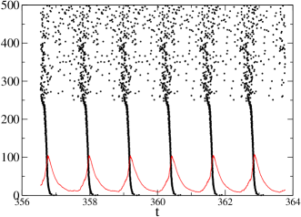
Figure 1: Raster plot representation of the dynamics of a network of $N=500$ neurons with a Gaussian in-degree distribution $P(\tilde{k})$ ($\langle\tilde{k}\rangle=0.7$, $\sigma_{\tilde{k}}=0.077$). Black dots signal single firing events of neurons at time $t$. Neurons are naturally ordered along the vertical axis according to the values of their in-degree. The global field $Y(t)$ (red line) is superposed to the raster plot for comparison (its actual values are multiplied by the factor $10^{3}$, to make it visible on the vertical scale).

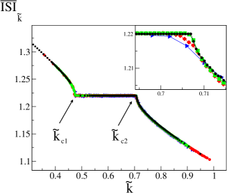
Figure 2: Time average of inter-spike intervals $\overline{ISI}({\tilde{k}})$ vs $\tilde{k}$ from a Gaussian distribution with $\langle\tilde{k}\rangle=0.7$ and $\sigma_{\tilde{k}}=0.077$ and for three networks with $N=500$ (blue triangles), $N=5000$ (red diamonds), $N=20000$ (green squares). For each size, the average is taken over 8 different realizations of the random network. We have also performed a suitable binning over the values of $\tilde{k}$, thus yielding the numerical estimates of the critical values $\tilde{k}_{c1}\approx 0.49$ and $\tilde{k}_{c2}\approx 0.70$. In the inset we show a zoom of the crossover region close to $\langle\tilde{k}\rangle=0.7$. Black dots are the result of simulations of the mean field dynamics (see Eq.s (6) – (8)) with $M=307$.

Heterogeneous Mean Field equations

We can now construct the Heterogeneous Mean–Field (HMF) equations for our model by combining this thermodynamic limit procedure with a consistency relation in Eqs. (2) - (4). The input field received by neuron $i$ is $Y_{i}=1/N\sum_{j}\epsilon_{ij}y_{j}(t)=1/N\sum_{j\in I(i)}y_{j}$, where $I(i)$ is the set of $k_{i}$ neurons transmitting to neuron $i$. For very large values of $N$ the average field generated by presynaptic neurons of neuron $i$, i.e. $1/k_{i}\sum_{j\in I(i)}y_{j}$, can be approximated with $1/N\sum_{j}y_{j}$, where the second sum runs over all neurons in the network (mean–field hypothesis). Accordingly, we have $Y_{i}=(k_{i}/N)(1/k_{i})\sum_{j\in I(i)}y_{j}\approx\tilde{k}_{i}(1/N\sum_{j}y_{j})$: as a consequence in the thermodynamic limit the dynamics of each neuron depends only on its specific in–degree. In this limit, $\tilde{k}_{i}$ becomes a continuous variable independent of the label $i$, taking values in the interval (0,1]. Therefore, all neurons with the same in–degree $\tilde{k}$ follow the same dynamical equations and we can write the dynamical equations for the class of neurons with in–degree $\tilde{k}$. Finally, we can replace $Y_{i}$ with $\tilde{k}Y(t)$, where

$$Y(t)=\int_{0}^{1}P(\tilde{k})y_{\tilde{k}}(t)d\tilde{k}$$ (5)

The HMF equations, then, read

$$\dot{v}_{\tilde{k}}(t)=a-v_{\tilde{k}}(t)+g\tilde{k}Y(t)$$ (6)

$$\dot{y}_{\tilde{k}}(t)=-\frac{y_{\tilde{k}}(t)}{\tau_{\mathrm{in}}}+u(1-y_{\tilde{k}}(t)-z_{\tilde{k}}(t))S_{\tilde{k}}(t)$$ (7)

$$\dot{z}_{\tilde{k}}(t)=\frac{y_{\tilde{k}}(t)}{\tau_{\mathrm{in}}}-\frac{z_{\tilde{k}}(t)}{\tau_{\mathrm{r}}}\,\,\,,$$ (8)

where $v_{\tilde{k}}$, $y_{\tilde{k}}$ and $z_{\tilde{k}}$ are the membrane potential, fraction of active and inactive resources of the class of neurons with in–degree $\tilde{k}$, respectively. Despite this set of equations cannot be solved explicitly, they provide a great numerical advantage with respect to direct simulations of large systems. Actually, the basic features of the dynamics of such systems can be effectively reproduced (modulo finite–size corrections) by exploiting a suitable sampling of $P(\tilde{k})$. For instance, one can sample the continuous variable $\tilde{k}\in[0,1]$ into $M$ discrete values $\tilde{k}_{i}$ in such a way that $\int_{\tilde{k}_{i}}^{\tilde{k}_{i+1}}P(\tilde{k})d\tilde{k}$ is kept fixed (importance sampling). Simulations of Equations (5)-(8) show that the global field field $Y(t)$ is periodic and the neurons split into locked and unlocked. Locked neurons feature a firing time delay with respect the peak of $Y(t)$, and this phase shift depends on the in–degree $\tilde{k}$. As to unlocked neurons, that typically have an in-degree $\tilde{k}>\langle\tilde{k}\rangle$, they follow a complex dynamics with irregular firing times. In Fig. 2 (black dots) we compare $\overline{ISI}(\tilde{k})$, obtained from the HMF equations for $M=307$, with the same quantity computed by direct simulations of networks up to size $N=2\times 10^{4}$. The agreement is remarkable evidencing the numerical effectiveness of the method.

The direct problem: stability analysis and the synchronization transition

In the HMF equations, once the global field $Y(t)$ is known, the dynamics of each class of neurons with in-degree $\tilde{k}$ can be determined by a straightforward integration, and we can perform the stability analysis that Tsodyks et al. applied to a similar model tso_locked . As an example, we have considered the system studied in Fig.2. The global field $Y(t)$ of the HMF dynamics has been obtained using the importance sampling for the distribution $P(\tilde{k})$. We have fitted $Y(t)$ with an analytic function of time $Y_{f}(t)$, continuous and periodic in time, with period $T$. Accordingly, Eq. (6) can be approximated by

$$\dot{v}_{\tilde{k}}(t)=a-v_{\tilde{k}}(t)+g\tilde{k}Y_{f}(t).$$ (9)

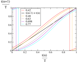
Figure 3: The return map $R_{\tilde{k}}$ in Eq. (10) of the rescaled variables $t_{\tilde{k}}(n)/T$ for different values of $\tilde{k}$, corresponding to lines of different colors, according to the legend in the inset: the black line is the bisector of the square.

Notice that, by construction, the field $Y_{f}(t)$ features peaks at times $t=nT$, where $n$ is an integer. In this way we can represent Eq. (9) as a discrete single neuron map. In practice, we integrate Eq.(9) and determine the sequence of the (absolute value of the) firing time–delay, $t_{\tilde{k}}(n)$, of neurons with in–degree $\tilde{k}$ with respect to the reference time $nT$. The return map $R_{\tilde{k}}$ of this quantity reads

$$t_{\tilde{k}}(n+1)=R_{\tilde{k}}t_{\tilde{k}}(n).$$ (10)

In Fig. 3 we plot the return map of the rescaled firing time–delay $t_{\tilde{k}}(n)/T$ for different values of $\tilde{k}$. We observe that in-degrees $\tilde{k}$ corresponding to locked neurons (e.g., the brown curve) have two fixed points $t_{\tilde{k}}^{s}$ and $t_{\tilde{k}}^{u}$, i.e. two points of intersection of the curve with the diagonal. The first one is stable (the derivative of the map $R_{\tilde{k}}$ is ¡ 1 ) and the second unstable (the derivative of the map $R_{\tilde{k}}$ is ¿ 1). Clearly, the dynamics converges to the stable fixed point displaying a periodic behavior. In particular, the firing times of neurons $\tilde{k}$ are phase shifted of a quantity $t_{\tilde{k}}^{s}$ with respect the peaks of the fitted global field. The orange and violet curves correspond to the dynamics at the critical in-degrees $\tilde{k}_{c1}$ and $\tilde{k}_{c2}$ where the fixed points disappear (see Fig.(2)). The presence of such fixed points influences also the behavior of the unlocked component (e.g., the red and light blue curves). In particular, the nearer $\tilde{k}$ is to $\tilde{k}_{c1}$ or to $\tilde{k}_{c2}$, the closer is the return map to the bisector of the square, giving rise to a dynamics spending longer and longer times in an almost periodic firing. Afterwards, unlocked neurons depart from this almost periodic regime, thus following an aperiodic behavior. As a byproduct, this dynamical analysis allows to estimate the values of the critical in–degrees. For the system of Fig.1$,\tilde{k}_{c1}=0.48$ and $\tilde{k}_{c2}=0.698$, in very good agreement with the numerical simulations (see Fig. 2).

Still in the perspective of the direct problem, the HMF equations provide further insight on how the network topology influences the dynamical behavior. We have found that, in general, the fraction of locked neurons increases as $P(\tilde{k})$ becomes sharper and sharper, while synchronization is eventually lost for broader distributions. In Fig. 4 we report the fraction of locked neurons, $f_{l}=\int_{\tilde{k}_{c1}}^{\tilde{k}_{c2}}P(\tilde{k})d\tilde{k}$, as a function of the standard deviation deviation $\sigma_{\tilde{k}}$, for different kinds of $P(\tilde{k})$ (single or double–peaked Gaussian, power law) in the HMF equations. For the truncated power law distribution, we set $P(\tilde{k})\sim\theta(\tilde{k}-\tilde{k}_{\mathrm{min}})\tilde{k}^{-\alpha}$. In all cases, there is a critical value of $\sigma_{\tilde{k}}$ above which $f_{l}$ vanishes, i.e. QSE disappear. The generality of this scenario points out the importance of the relation between $P(\tilde{k})$ and the average synaptic field $Y(t)$.

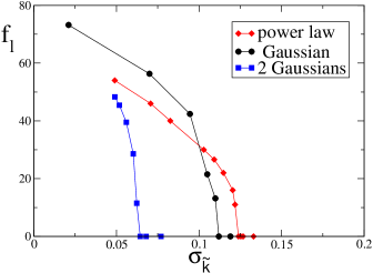
Figure 4: The fraction of locked neurons, $f_{l}$, as a function of the standard deviation $\sigma_{\tilde{k}}$ of the distributions: truncated Gaussian with $\langle\tilde{k}\rangle=0.7$ (black dots); truncated superposition of two Gaussians (both with standard deviation 0.03), one centered at $\tilde{k}_{1}=0.5$ and the other one at a varying value $\tilde{k}_{2}$, that determines the overall standard deviation $\sigma_{\tilde{k}}$ (blue squares); truncated power law distribution with $\tilde{k}_{\mathrm{min}}=0.1$ (red diamonds). In the last case the value of the standard deviation is changed by varying the exponent $\alpha$, while the average $\langle\tilde{k}\rangle$ changes accordingly. Lines have been drawn to guide the eyes.

The inverse problem

The HMF approach allows to implement the inverse problem and leads to the reconstruction of the distribution $P(\tilde{k})$ from the knowledge of $Y(t)$. If the global synaptic activity field $Y(t)$ is known, each class of neurons of in-degree $\tilde{k}$ evolves according to the equations:

$$\dot{\mathsf{v}}_{\tilde{k}}(t)=a-\mathsf{v}_{\tilde{k}}(t)+g\tilde{k}Y(t)$$ (11)

$$\dot{\mathsf{y}}_{\tilde{k}}(t)=-\frac{\mathsf{y}_{\tilde{k}}(t)}{\tau_{\mathsf{in}}}+u(1-\mathsf{y}_{\tilde{k}}(t)-\mathsf{z}_{\tilde{k}}(t))\tilde{S}_{\tilde{k}}(t)$$ (12)

$$\dot{\mathsf{z}}_{\tilde{k}}(t)=\frac{\mathsf{y}_{\tilde{k}}(t)}{\tau_{\mathsf{in}}}-\frac{\mathsf{z}_{\tilde{k}}(t)}{\tau_{\mathsf{r}}}\,\,\,.$$ (13)

Notice that the variable $\mathsf{v}(t)$, $\mathsf{y}(t)$, $\mathsf{z}(t)$ can take values that differ from the variables generating the field $Y(t)$, i.e. $v(t)$, $y(t)$, $z(t)$, as they start from different initial conditions. However, the self consistent relation for the global field $Y(t)$ implies:

$$Y(t)=\int_{0}^{1}P({\tilde{k}})\mathsf{y}_{\tilde{k}}(t)d{\tilde{k}}\,\,\,.$$ (14)

If $Y(t)$ and $\mathsf{y}_{\tilde{k}}(t)$ are known, this is a Fredholm equation of the first kind in $P(\tilde{k})$ kress . In the general case of Eq. (1), calling $E(t)$ the global measured external field, the evolution equations corresponding to Eq.s (11)–(13) read

$${\dot{\mathbf{w}}_{\tilde{k}}}=\mathbf{F}\Big{(}{\mathbf{w}}_{\tilde{k}},g\tilde{k}E(t)\Big{)}\,$$ (15)

and the Fredholm equation for the inverse problem is

$$E(t)=\int_{0}^{1}P(\tilde{k})G({\mathbf{w}}_{\tilde{k}}(t))d\tilde{k}\,\,\,.$$ (16)

In the case of our LIF model, as soon as a locked component exists, Eq. (14) can be solved by a functional Montecarlo minimization procedure applied to a sampled $P(\tilde{k})$. At variance with the direct problem, $P(\tilde{k})$ is the unknown function and, accordingly, we have to adopt a uniform sampling of the support of $\tilde{k}$. A sufficiently fine sampling has to be used for a confident reconstruction of $P(\tilde{k})$ (See Methods section).

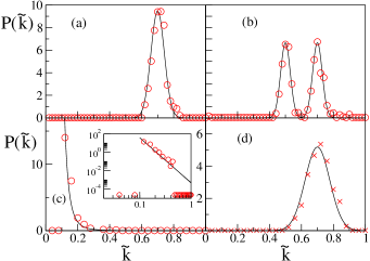
Figure 5: Inverse problem for $P(\tilde{k})$ from the global field $Y(t)$. Panels (a), (b) and (c) show three distributions of the kind considered in Fig. (4) (black continuous curves) for the HMF equations and their reconstructions (circles) by the inverse method. The parameters of the three distributions are $\sigma_{\tilde{k}}=0.043$, $\tilde{k}_{2}=0.7$ and $\alpha=4.9$. In panel (d) we show the reconstruction (crosses) of $P(\tilde{k})$ (black continuous line) by the average field $Y(t)$ generated by the dynamics of a finite size network with $N=500$.

To check our inverse method, we choose a distribution $P(\tilde{k})$, evolve the system and extract the global synaptic field $Y(t)$. We then verify if the procedure reconstructs correctly the original distribution $P(\tilde{k})$. In panels (a), (b) and (c) of Fig. 5 we show examples in which $Y(t)$ has been obtained from the simulation of the HMF with different $P(\tilde{k})$ (Gaussian, double peak Gaussian and power law). We can see that the method determines confidently the original distribution $P(\tilde{k})$. Notice that the method fails as soon as the locked component disappears, as explained in the methods section. Remarkably, the method can recognize the discontinuity of the distribution in $\tilde{k}=\tilde{k}_{\mathrm{min}}$ and the value of the exponent of the power law $\alpha=4.9$. Finally, in panel (d) of Fig.5, we show the result of the inverse problem for the distribution $P(\tilde{k})$ obtained from a global signal generated by a finite size realization with $N=500$ and $\langle k\rangle=350$. The significant agreement indicates that the HMF and its inverse problem are able to infer the in–degree probability distribution $P(\tilde{k})$ even for a realistic finite size network. This last result is particularly important, as it opens new perspectives for experimental data analysis, where the average neural activity is typically measured from finite size samples with finite but large connectivity.

Discussion

The direct and inverse problem for neural dynamics on random networks are both accessible through the HMF approach proposed in this paper. The mean-field equations provide a semi–analytic form for the return map of the firing times of neurons and they allow to evidence the effects of the in-degree distribution on the synchronization transition. This phenomenology is not limited to the LIF model analyzed here and it is observed in several neural models on random networks. We expect that the HMF equations could shed light on the nature of this interesting, but still not well understood, class of synchronization transitions ps ; olmi ; luccioli . The mean field nature of the approach does not represent a limitation, since the equations are expected to give a faithful description of the dynamics also in networks with finite but large average in-degree, corresponding to the experimental situation observed in many cortical regions kgrande .

The inverse approach, although tested here only on numerical experiments, gives excellent results on the reconstruction of a wide class of in-degree distributions and it could open new perspectives on data analysis, allowing to reconstruct the main topological features of the neural network producing the QSE. The inversion appears to be stable with respect to noise, as clearly shown by the effectiveness of the procedure tested on a finite realization, where the temporal signals of the average synaptic activity is noisy. We also expect our inverse approach to be robust with respect to the addition of limited randomness in leaky currents, and also with respect to a noise compatible with the signal detection from instruments. Finally, the method is very general and it can be applied to a wide class of dynamical models on networks, as those described in Eq. (1).

Further developments will allow to get closer to real experimental situations. We mention the most important, i.e. the introduction of inhibitory neurons and the extension of our approach by taking into account networks with degree correlations mendes , that are known to characterize real structures, and sparse networks. The HMF equations appear to be sufficiently flexible and simple to allow for these extensions.

Methods

Montecarlo approach to the inverse problem

In this section we provide details of the algorithmic procedure adopted for solving the inverse problem, i.e. reconstructing the distribution $P(\tilde{k})$ from Eq. (14). In the HMF formulation, the field $Y(t)$ is generated by an infinite number of neurons and $\tilde{k}$ is a continuous variable in the interval $(0,1]$. In practice, we can sample uniformly this unit interval by $L$ disjoint subintervals of length $1/L$, labelled by the integer $i$. This corresponds to an effective neural index $i$, that identifies the class of neurons with in-degree $\tilde{k}_{i}=i/L$. In this way we obtain a discretized definition converging to Eq.(14) for $L\to\infty$:

$$Y(t)=\int_{0}^{1}P(\tilde{k})\mathsf{y}_{\tilde{k}}(t)d\tilde{k}\simeq\frac{1}{L}\sum_{i=0}^{L-1}P(\tilde{k}_{i})\mathsf{y}_{\tilde{k}_{i}}(t)\,\,.$$ (17)

In order to improve the stability and the convergence of the algorithm by smoothing the fluctuations of the fields $\mathsf{y}_{\tilde{k}_{i}}(t)$, it is convenient to consider a coarse–graining of the sampling by approximating $Y(t)$ as follows

$$Y(t)=\frac{1}{L^{\prime}}\sum_{i=0}^{L^{\prime}-1}P(\tilde{k}_{i})\langle\mathsf{y}_{\tilde{k}_{i}}(t)\rangle.$$ (18)

where $\langle\mathsf{y}_{\tilde{k}_{i}}(t)\rangle$ is the average of $L/L^{\prime}$ synaptic fields of connectivity $\tilde{k}\in[{\tilde{k}_{i}},{\tilde{k}_{i+1}}]$. This is the discretized Fredholm equation that one can solve to obtain $P(\tilde{k}_{i})$ from the knowledge of $\langle\mathsf{y}_{\tilde{k}_{i}}(t)\rangle$ and $Y(t)$. For this aim we use a Monte Carlo (MC) minimization procedure, by introducing at each MC step, $n$, a trial solution, $P_{n}(\tilde{k}_{i})$, in the form of a normalized non-negative in-degree distribution. Then, we evaluate the field $Y_{n}(t)$ and the distance $\gamma_{n}$ defined as:

$$Y_{n}(t,P_{n}(\tilde{k}_{i})) =\frac{1}{L^{\prime}}\sum_{i=0}^{L^{\prime}-1}P_{n}(\tilde{k}_{i})\langle\mathsf{y}_{\tilde{k}_{i}}(t)\rangle$$ (19)

$$\gamma_{n}(P_{n}(\tilde{k}_{i}))^{2} =\frac{1}{t_{2}-t_{1}}\int_{t_{1}}^{t_{2}}\frac{\Big{[}Y_{n}(t,P_{n}(\tilde{k}_{i}))-Y(t))\Big{]}^{2}}{Y^{2}(t)}dt\,\,\,.$$ (20)

The time interval $[t_{1},t_{2}]$ has to be taken large enough to obtain a reliable estimate of $\gamma_{n}$. For instance, in the case shown in Fig.1, where $Y(t)$ exhibits an almost periodic evolution of period $T\approx 1$ in the adimensional units of the model, we have used $t_{2}-t_{1}=10$. The overall configuration of the synaptic fields, at iteration step $n+1$, is obtained by choosing randomly two values $\tilde{k}_{j}$ and $\tilde{k}_{l}$, and by defining a new trial solution $\bar{P}_{n+1}(\tilde{k})=P_{n}(\tilde{k})+\epsilon\delta_{\tilde{k},\tilde{k}_{j}}-\epsilon\delta_{\tilde{k},\tilde{k}_{l}}$, so that, provided both $\bar{P}_{n+1}(\tilde{k}_{j})$ and $\bar{P}_{n+1}(\tilde{k}_{l})$ are non-negative, we increase and decrease $P_{n}(\tilde{k}_{j})$ of the same amount, $\epsilon$, in $\tilde{k}_{j}$ and $\tilde{k}_{l}$ respectively. A suitable choice is $\epsilon\sim\mathcal{O}(10^{-4})$. Then, we evaluate $\gamma_{n+1}(\bar{P}_{n+1}(\tilde{k}_{i}))$: If $\gamma_{n+1}(\bar{P}_{n+1}(\tilde{k}_{i}))<\gamma_{n}({P}_{n}(\tilde{k}_{i}))$ the step is accepted i.e. $P_{n+1}=\bar{P}_{n+1}$, otherwise $P_{n+1}=P_{n}$. This MC procedure amounts to the implementation of a zero temperature dynamics, where the cost function $\gamma_{n}({P}_{n}(\tilde{k}_{i}))$ can only decrease. In principle, the inverse problem in the form of Eq.(18) is solved, i.e. $Y_{n}(t,P_{n}(\tilde{k}_{i}))=Y(t)$, if $\gamma_{n}({P}_{n}(\tilde{k}_{i}))=0$. In practice, the approximations introduced by the coarse-graining procedure do not allow for a fast convergence to the exact solution, but $P_{n}(\tilde{k}_{i})$ can be considered a reliable reconstruction of the actual $P(\tilde{k})$ already for $\gamma_{n}<10^{-2}$. We have checked that the results of the MC procedure are quite stable with respect to different choices of the initial conditions ${P}_{0}(\tilde{k}_{i})$, thus confirming the robustness of the method. We give in conclusion some comments on the very definition of the coarse-grained synaptic field $\langle\mathsf{y}_{\tilde{k}_{i}}(t)\rangle$. Since small differences in the values of $\tilde{k}_{i}$ reflect in small differences in the dynamics, for not too large intervals $[{\tilde{k}_{i}},{\tilde{k}_{i+1}}]$ the quantity $\langle\mathsf{y}_{\tilde{k}_{i}}(t)\rangle$ can be considered as an average over different initial conditions. For locked neurons the convergence of the average procedure defining $\langle\mathsf{y}_{\tilde{k}_{i}}(t)\rangle$ is quite fast, since all the initial conditions tend to the stable fixed point, identified by the return map described in the previous subsection. On the other hand, the convergence of the same quantity for unlocked neurons should require an average over a huge number of initial conditions. For this reason, the broader is the distribution, i.e. the bigger is the unlocked component (see Fig.4), the more computationally expensive is the solution of the inverse problem. This numerical drawback for broad distributions emerges in our tests of the inversion procedure described in Fig. 5. Moreover, such tests show that the procedure works insofar the QSE are not negligible, but it fails in the absence of the locking mechanism. In this case, indeed, the global field $Y(t)$ is constant and also $\langle\mathsf{y}_{\tilde{k}_{i}}(t)\rangle$ become constant, when averaging over a sufficiently large number of samples. This situation makes Eq.(18) trivial and useless to evaluate $P(\tilde{k}_{i})$. We want to observe that, while in general $\mathsf{y}_{\tilde{k}_{i}}(t)\not=y_{\tilde{k}_{i}}(t)$, one can reasonably expect that $\langle\mathsf{y}_{\tilde{k}_{i}}(t)\rangle$ is a very good approximation of $\langle y_{\tilde{k}_{i}}(t)\rangle$. This remark points out the conceptual importance of the HMF formulation for the possibility of solving the inverse problem.

Additional Information

Author contribution statement

R. B., M. C., M. d. V., R. L., A, V. contributed to the formulation of the problem, to its solution, to the discussions, and to the writing of the paper. M. d. V. performed the simulations and produced all the plots.

Competing financial interests

The authors declare no competing financial interests.

I Captions

Fig. 1: Raster plot representation of the dynamics of a network of $N=500$ neurons with a Gaussian in-degree distribution $P(\tilde{k})$ ($\langle\tilde{k}\rangle=0.7$, $\sigma_{\tilde{k}}=0.077$). Black dots signal single firing events of neurons at time $t$. Neurons are naturally ordered along the vertical axis according to the values of their in-degree. The global field $Y(t)$ (red line) is superposed to the raster plot for comparison (its actual values are multiplied by the factor $10^{3}$, to make it visible on the vertical scale).

Fig. 2: Time average of inter-spike intervals $\overline{ISI}({\tilde{k}})$ vs $\tilde{k}$ from a Gaussian distribution with $\langle\tilde{k}\rangle=0.7$ and $\sigma_{\tilde{k}}=0.077$ and for three networks with $N=500$ (blue triangles), $N=5000$ (red diamonds), $N=20000$ (green squares). For each size, the average is taken over 8 different realizations of the random network. We have also performed a suitable binning over the values of $\tilde{k}$, thus yielding the numerical estimates of the critical values $\tilde{k}_{c1}\approx 0.49$ and $\tilde{k}_{c2}\approx 0.70$. In the inset we show a zoom of the crossover region close to $\langle\tilde{k}\rangle=0.7$. Black dots are the result of simulations of the mean field dynamics (see Eq.s (6) – (8)) with $M=307$.

Fig. 3: The return map $R_{\tilde{k}}$ in Eq. (10) of the rescaled variables $t_{\tilde{k}}(n)/T$ for different values of $\tilde{k}$, corresponding to lines of different colors, according to the legend in the inset: the black line is the bisector of the square.

Fig. 4: The fraction of locked neurons, $f_{l}$, as a function of the standard deviation $\sigma_{\tilde{k}}$ of the distributions: truncated Gaussian with $\langle\tilde{k}\rangle=0.7$ (black dots); truncated superposition of two Gaussians (both with standard deviation 0.03), one centered at $\tilde{k}_{1}=0.5$ and the other one at a varying value $\tilde{k}_{2}$, that determines the overall standard deviation $\sigma_{\tilde{k}}$ (blue squares); truncated power law distribution with $\tilde{k}_{\mathrm{min}}=0.1$ (red diamonds). In the last case the value of the standard deviation is changed by varying the exponent $\alpha$, while the average $\langle\tilde{k}\rangle$ changes accordingly. Lines have been drawn to guide the eyes.

Fig. 5: Inverse problem for $P(\tilde{k})$ from the global field $Y(t)$. Panels (a), (b) and (c) show three distributions of the kind considered in Fig. (4) (black continuous curves) for the HMF equations and their reconstructions (circles) by the inverse method. The parameters of the three distributions are $\sigma_{\tilde{k}}=0.043$, $\tilde{k}_{2}=0.7$ and $\alpha=4.9$. In panel (d) we show the reconstruction (crosses) of $P(\tilde{k})$ (black continuous line) by the average field $Y(t)$ generated by the dynamics of a finite size network with $N=500$.

References

- (1) Wang, X.F. Synchronization in small-world dynamical networks, Int. J. Bifurcation Chaos 12, 885 (2002).
- (2) Barrat, A., Barthelemy, M. & Vespignani, A. Dynamical Processes on Complex Networks, Cambridge University Press, Cambridge, UK (2008).
- (3) Dorogovtsev, S.N., Goltsev, A.V. & Mendes, J.F.F. Critical phenomena in complex networks, Rev. Mod. Phys. 80, 1275 (2008).
- (4) Cohen, R. & Havlin,S. Complex Networks: Structure, Robustness and Function, Cambridge University Press, Cambridge, UK, (2010).
- (5) Arenas, A., Díaz-Guilera, Kurths, J., Moreno, Y. & Zhou, C. Synchronization in complex networks, Phys. Rep. 469, 93 (2008).
- (6) Boccaletti, S., Latora, V., Moreno, Y., Chavez, M. & Hwanga, D.U., Complex networks: Structure and dynamics Phys. Rep. 424, 175 (2006).
- (7) Donetti, L., Hurtado, P.I. & Muoz, M.A., Entangled networks, synchronization, and optimal network topology, Phys. Rev. Lett. 95, 188701 (2005).
- (8) Shneidman, E., Berry, M.J., Segev, R. & Bialek, W. Weak pairwise correlations imply strongly correlated network states in a neural population, Nature 440, 1007 (2006)
- (9) Cocco, S., Leibler, S. & Monasson, R. Neuronal couplings between retinal ganglion cells inferred by efficient inverse statistical physics methods, R. Proc. Natl. Acad. Sci. U.S.A. 106, 14058 (2009).
- (10) Shandilya, S.G. & Timme, M. Inferring network topology from complex dynamics, New J. Phys. 13, 013004 (2011).
- (11) Zheng, H.L., Alava, M., Aurell, E., Hertz, J. & Roudi, Y. Maximum likelihood reconstruction for Ising models with asynchronous updates, Phys. Rev. Lett. 110, 210601 (2013).
- (12) Niedermeyer, E. & Lopes da Silva, F.H. Electroencephalography: Basic Principles, Clinical Applications, and Related Fields, Lippincott Williams & Wilkins, (2005).
- (13) Huettel, S.A., Song, A.W. & McCarthy, G. Functional Magnetic Resonance Imaging, Sunderland, MA: Sinauer Associates, (2009).
- (14) Tsodyks, M. & Markram, H. The neural code between neocortical pyramidal neurons dependson neurotransmitter release probability, Proc. Natl. Acad. Sci. USA 94, 719 (1997).
- (15) Tsodyks, M., Pawelzik, K. & Markram, H. Neural networks with dynamic synapses, Neural Comput. 10, 821, (1998).
- (16) Tsodyks, M., Uziel, A. & Markram, H. Synchrony Generation in Recurrent Networks withFrequency-Dependent Synapses, The Journal of Neuroscience, 20, RC1 (1-5) (2000).
- (17) Volman, V., Baruchi, I., Persi, E. & Ben-Jacob, Generative modelling of regulated dynamical behavior in cultured neuronal networks, E. Physica A 335, 249 (2004).
- (18) di Volo, M. & Livi, R. The influence of noise on synchronous dynamics in a diluted neural network, J. of Chaos Solitons and Fractals 57, 54–61 (2013).
- (19) di Volo, M., Livi, R., Luccioli, S., Politi, A. & Torcini, A. Synchronous dynamics in the presence of short-term plasticity, Phys. Rev. E 87, 032801 (2013).
- (20) Chung, F., Lu, L. Complex Graphs and Networks, CBMS Series in Mathematics, AMS (2004).
- (21) Pastor-Satorras, R. & Vespignani, A. Epidemic spreading in scale-free networks. Phys. Rev. Lett. 86, 3200 (2001).
- (22) A. Vespignani, Modelling dynamical processes in complex socio-technical systems Nature Physics 8, 39 (2012).
- (23) Kress, R. Linear Integral equations, Applied numerical sciences, 82, Springer-Verlag, New York, (1999).
- (24) Olmi, S., Livi, R., Politi, A. & Torcini, A. Collective oscillations in disordered neural networks, Phys. Rev. E 81 046119 (2010).
- (25) Luccioli, S., Olmi, S., Politi, A. & Torcini, A. Collective dynamics in sparse networks, A. Phys. Rev. Lett. 109, 138103 (2012).
- (26) Buzsaki, G., Rhythms of the Brain, Oxford University Press, New York (2006).
- (27) Richardson Magnus J. E., Brunel N. and Hakim V. From Subthreshold to Firing-Rate Resonance, J Neurophysiol 89, 2538 2554, (2003).
- (28) Brette, R. Exact simulation of integrate–and–fire models with synaptic conductances, Neural Comput. 18, 2004 (2006).
- (29) Zillmer, R., Livi, R., Politi, A. & Torcini, A. Stability of the splay state in pulse-coupled networks, Phys. Rev. E 76, 046102 (2007).
- (30) Tsodyks, M., Mitkov, I. & Sompolinsky, H. Pattern of synchrony in inhomogeneous networks of oscillators with pulse interactions, Phys. Rev. Lett. 71, 1280 (1993).
- (31) Mohanty, P.K. & Politi A. A new approach to partial synchronization in globally coupled rotators, J. Phys. A: Math. Gen. 39 L415-L421 (2006).
- (32) Deco G., Ponce-Alvarez A., Mantini D., Romani G.L., Hagmann P., Corbetta M. Resting-State Functional Connectivity Emerges from Structurally and Dynamically Shaped Slow Linear Fluctuations, The Journal of Neuroscience, 33(27), 11239 (2013).
Acknowledgements
This work is partially supported by the Centro Interdipartimentale per lo Studio delle Dinamiche Complesse (CSDC) of the Universita’ di Firenze, and by the Istituto Nazionale di Fisica Nucleare (INFN).