Accelerating inference for diffusions observed with measurement error and large sample sizes using Approximate Bayesian Computation

Abstract

In recent years dynamical modelling has been provided with a range of breakthrough methods to perform exact Bayesian inference. However it is often computationally unfeasible to apply exact statistical methodologies in the context of large datasets and complex models. This paper considers a nonlinear stochastic differential equation model observed with correlated measurement errors and an application to protein folding modelling. An Approximate Bayesian Computation (ABC) MCMC algorithm is suggested to allow inference for model parameters within reasonable time constraints. The ABC algorithm uses simulations of “subsamples” from the assumed data generating model as well as a so-called “early rejection” strategy to speed up computations in the ABC-MCMC sampler. Using a considerate amount of subsamples does not seem to degrade the quality of the inferential results for the considered applications. A simulation study is conducted to compare our strategy with exact Bayesian inference, the latter resulting two orders of magnitude slower than ABC-MCMC for the considered setup. Finally the ABC algorithm is applied to a large size protein data. The suggested methodology is fairly general and not limited to the exemplified model and data.

Keywords: likelihood-free inference, MCMC, protein folding, stochastic differential equation.

1 Introduction

In the so-called “Big Data” era we face the need and the opportunity to extract information provided by a steadily increasing amount of data, as produced by e.g. in-silico and in-vivo experiments, to describe real-world systems at previously unattainable resolutions. As the size of datasets requiring analysis increases, so must the statistical techniques used to analyse them be able to efficiently handle the increase in scale. Standard statistical approaches, both classical and Bayesian, were not designed with this in mind and statisticians now have to consider models of adequate complexity while trying to obtain inferential results within reasonable time limits.

In recent years statistical inference for dynamical modelling has been provided with powerful tools to perform exact inference on models of considerable complexity, thanks to sequential Monte Carlo methods embedded within Markov chain Monte Carlo (MCMC) algorithms Andrieu et al. (2010) as well as “likelihood-free” methods Bretó et al. (2009); Golightly and Wilkinson (2011), see section 3 for more details. Such methods have flourished in the Bayesian community and have pushed the exploration for possibilities previously unrealistic to contemplate. However these computational methods usually don’t scale well enough to match the increasing sizes of datasets. In this work we exemplify inference for a stochastic dynamical model describing protein dynamics time series data approximately of size 25,000, and even if such size is not large enough to be considered a typical example of “Big Data”, it has been a challenge for us to perform inference for a particular nonlinear stochastic differential equation (SDE) model observed with correlated measurement error. The use of exact methods in our application was not feasible, without reverting to a rather arbitrary subsample of the available data. Similar difficulties are expected in applications in systems biology and bioinformatics.

Here we present a strategy to rely on the full data-set without having to simulate trajectories for the latent process of the same size as the data. The considered inferential framework is approximate Bayesian computation (ABC) within an MCMC algorithm, where acceptance of simulated trajectories and corresponding generating parameters is regulated by the use of specific “summary statistics”. When the chosen summary statistics applied on (relatively short) simulated trajectories approximately match the summary statistics for the (much larger) observed dataset, the proposed parameter has a higher probability to be accepted. This mechanism thus enable approximate inference for arbitrarily large datasets, as the summary statistics for the real data need to be computed only once, whereas during the ABC-MCMC algorithm statistics for simulated datasets are relatively cheap to compute, due to the shorter size of the artificial trajectories. An analysis of protein folding data is presented, based on a recent model expressed as a sum of two diffusion processes Forman and Sørensen (2014), hereafter denoted “diffusion observed with measurement error”. Inference via ABC is performed on such data. A simulation study for a smaller dataset is also performed, comparing ABC against exact inference obtained via particle MCMC methods (Andrieu et al., 2010).

2 Diffusion observed with measurement error

As an example of a fairly complex dynamical model, we consider a nonlinear diffusion model observed with measurement error. The model was introduced by Forman and Sørensen (2014) to model the dynamics of a particular protein folding problem which is further investigated in section 6. The stationary distribution of the nonlinear diffusion is bimodal in order to reflect the two regimes of the protein, folded and unfolded. To be specific, let the observable stochastic process $\{Z_{t}\}$ be defined by

$$\begin{cases}Z_{t}=\tau_{\psi}(X_{t})+U_{t},\qquad t\geq t_{0}\\ dU_{t}=-\kappa U_{t}dt+\sqrt{2\kappa\gamma^{2}}dW_{t},\qquad U_{t_{0}}=0\\ dX_{t}=-\theta X_{t}dt+\sqrt{2\theta}dB_{t},\qquad X_{t_{0}}=x_{t_{0}}\\ \end{cases}$$ (1)

where the error process $\{U_{t}\}$ is a Ornstein-Uhlenbeck (OU) process with stationary mean zero, stationary variance $\gamma^{2}$ and autocorrelation function $\rho_{U}(t)=e^{-\kappa t}$, the latent process $\{X_{t}\}$ is yet another OU process with stationary mean zero, unit variance and autocorrelation function $\rho_{X}(t)=e^{-\theta t}$, $\{W_{t}\}$ and $\{B_{t}\}$ are independent Brownian motions. The transformation $\tau_{\psi}(\cdot)$ with ${\bm{\psi}}=(\alpha,\mu_{1},\mu_{2},\sigma_{1},\sigma_{2})$ is given by $\tau_{\psi}(x)=(F_{\psi}^{-1}\circ\Phi)(x)$ where

$$F_{\psi}(y)=\alpha\cdot\Phi\left(\frac{y-\mu_{1}}{\sigma_{1}}\right)+(1-\alpha)\cdot\Phi\left(\frac{y-\mu_{2}}{\sigma_{2}}\right)$$ (2)

and $\Phi(\cdot)$ denotes the cumulative distribution function of the standard normal distribution. Note that the transformation $\operatorname{\tau}_{\psi}(\cdot)$ maps the invariant $N(0,1)$-distribution of the OU-process $\{X_{t}\}$ to a bimodal mixture of normal distributions with modes at $\mu_{1}$ and $\mu_{2}$ and mixture parameter $\alpha\in(0,1)$. In other words, $\tau_{\psi}(X_{t})$ is the $\Phi(X_{t})$-percentile of the two-components Gaussian mixture having cumulative distribution function (2). It is important to notice that the model has a simple latent structure arising from the fact that both the error process $\{U_{t}\}$ and the nonlinear diffusion $\{X_{t}\}$ are OU processes, where one has been transformed to match the desired stationary distribution of the data. Recall that an OU process has Gaussian transition densities, for example for $\{X_{t}\}$ we have

$$X_{t}|X_{s}=x\sim N(x\cdot e^{-\theta\Delta_{t}},1-e^{-2\theta\Delta_{t}}),\quad\textnormal{ with }\Delta_{t}=t-s$$ (3)

for $s<t$. Further note that the process $\{Z_{t}\}_{t\geq 0}$ is able to display multi-scale behaviour. Whenever $0<\theta\ll\kappa$, the error process $\{U_{t}\}$ dominates the dynamics of the observable process on the short time scale, while the latent nonlinear diffusion $\{\tau_{\psi}(X_{t})\}$ determines the observed behaviour on the long time scale. We refer to Pavliotis and Stuart (2007); Azencott et al. (2013) for further discussion of multi-scale models and the difficulties related to performing statistical inference.

Please note that the statistical methodology discussed in this paper applies to a much wider range of processes than the exemplified model (1). In particular, the transformation could be replaced by one targeting other distributions than the bimodal normal mixture or the process $\{\tau_{\psi}(X_{t})\}$ could be replaced by an entirely different diffusion, e.g. a double-well potential model or a nonlinear diffusion model as considered by Aït-Sahalia (1996). More general partially observed and multi-scale diffusions such as the ones presented in Pokern et al. (2009); Crommelin and Vanden-Eijnden (2011) could also be considered. The motivation for choosing model (1) is due to the fact that it yields explicit formulae for the mean passage times, see Forman and Sørensen (2014), which are important for estimating the folding and unfolding rates of the protein data (section 6). From the perspective of the protein folding problem, the model has the further advantage that the nonlinear latent diffusion displays increased volatility inbetween the modes which is in accordance with the empirical finding of state-dependent diffusion in protein reaction coordinates, see Best and Hummer (2010). Finally, Forman and Sørensen (2014) found that the diffusion with error model was able to fit the protein data satisfactory both on the short and the long time scale, which was not the case with any plain diffusion model.

3 Issues with exact Bayesian inference

Consider the problem of making inference for the parameter ${\bm{\eta}}=(\theta,\kappa,\gamma,{\bm{\psi}})$ of the nonlinear diffusion with error model described in Section 2. Denote with ${\bm{z}}=\{z_{0},z_{1},\ldots,z_{n}\}$ a set of discrete observations from $\{Z_{t}\}$ and with ${\bm{x}}=\{x_{0},x_{1},\ldots,x_{n}\}$ corresponding unobserved values from $\{X_{t}\}$. The likelihood function of ${\bm{\eta}}$ based on ${\bm{z}}$ is

$$L({\bm{\eta}}) =p({\bm{z}}|{\bm{\eta}})=\prod_{i=1}^{n}p(z_{i}|z_{0},z_{1},...,z_{i-1};{\bm{\eta}})$$ (4)

$$=\int p(z_{0},...,z_{n}|\tau(x_{0}),...,\tau(x_{n});{\bm{\eta}})p(\tau(x_{0}),...,\tau(x_{n})|{\bm{\eta}})d\tau(x_{0})\cdots d\tau(x_{n})$$

$$=\int p(z_{0},...,z_{n}|\tau(x_{0}),...,\tau(x_{n}))\prod_{i=1}^{n}p(\tau(x_{i})|\tau(x_{i-1});{\bm{\eta}})d\tau(x_{0})\cdots d\tau(x_{n})$$

where the product in the last integrand is due to the Markov property of $\{X_{t}\}$. This likelihood function is neither explicitly known nor easy to approximate. For this reason we wish to consider a Bayesian approach for doing inference on ${\bm{\eta}}$. Unfortunately, as discussed below, several difficulties related to our specific application prevent using conventional exact methodology. Firstly, due to the autocorrelation in $\{U_{t}\}$, the observations ${\bm{z}}$ are not conditionally independent given the latent state ${\bm{x}}$. This obstructs the use of most methods available for state-space models (aka Hidden Markov Models). In Andrieu et al. (2010) it has been shown how to use sequential Monte Carlo (SMC) methods for a class of models larger than state-space models by use of the particle MCMC methodology. In principle, particle MCMC algorithms plug an SMC approximation to (4) into an MCMC procedure for inference on ${\bm{\eta}}$, state variables or both. When such approximation is an unbiased estimate of the likelihood we are rewarded with exact Bayesian inference, regardless the number of particles used in the SMC step. However, since in our case $n\approx 2.5\times 10^{4}$, this approach is not practically feasible as it would take several weeks of computation on our hardware, depending on the number of particles used. To be specific, we initially implemented particle MCMC approach with the adaptation suggested in Golightly and Wilkinson (2011), suitable for Bayesian inference for diffusion models. Even when using only 10 particles and writing our program in the Julia language (Bezanson et al., 2012) (in some cases comparable to C++ in terms of performance), the result was far too slow to be worthwhile. It has to be noted, though, that we have not exploited available GPUs implementations such as Murray (2013), which are likely to reduce the computational cost.

Without reverting to SMC methods, a class of methods that often gives satisfactory results is the one enabling so-called “likelihood-free” inference, see section 9.6 in Wilkinson (2012). This is sometimes referred to as “plug-and-play” Ionides et al. (2006); Bretó et al. (2009) as it bypasses the explicit calculation of the likelihood function by forward simulating from the data-generating model. Unfortunately the application of likelihood–free MCMC is not feasible in our “large data” context. Poor mixing is a well known problem in inference for diffusion models via MCMC as the underlying process is by nature very erratic. For large data sets such as the one exemplified in Section 6 it is very unlikely for a generated trajectory to be close enough to data to have the corresponding parameter proposal accepted. Low acceptance rates could be observed even when the value of ${\bm{\eta}}$ is in the bulk of the posterior distribution support. Another reason to expect inefficiency in forward simulations is when trajectories are generated unconditional on data. SMC methods offers an improvement in this regards by having the ability to assign larger weights to particles close to observed data, but we cannot use such approach as explained in the above.

An additional difficulty is related to the simulation of a sufficiently accurate trajectory for $\{\tau(X_{t})\}$. This is in general a non-issue for SDE models as many approximation schemes are available (Kloeden and Platen, 1992; Rößler, 2010). In our specific case numerical discretization is not even required as the process $\{X_{t}\}$ can be simulated exactly using the transition densities (3). Unfortunately, computing $\tau(X_{t})$ is not straightforward because we need to apply the quantile function of the Gaussian mixture distribution which does not have a closed–form expression. In practice, we get to solve a nonlinear optimization problem amounting to finding the zero point $Y_{t}=\tau(X_{t})$ of $f(\cdot,X_{t})=F_{\psi}(\cdot)-\Phi(X_{t})$ where $F_{\psi}$ is the cumulative distribution function defined by (2). The optimization must be repeated for any given sampling time $t_{i}$ ($i=1,...,n$) where in our case $n$ is large ($\approx 25,000$) and for any parameter value ${\bm{\eta}}$ occuring during the inferential procedure of choice. This is computationally very demanding even though the generation of the $\tau(X_{t})$’s can be considered virtually exact, as we control the precision of the approximated values from the numerical optimization.

Because of the many difficulties highlighted above we revert to approximate Bayesian computation, which offers a likelihood–free approach to treat complex stochastic models.

4 Approximate Bayesian computation

The attempt to model complete data sets has dominated the Bayesian methodology for decades. However, with the advent of large datasets and complex models this often turns challenging, if not impossible. Some recent attempts at speeding-up inference via MCMC using subsets of available data are presented by Girolami et al. (2013); Korattikara et al. (2014) and the references therein. Aside from the Bayesian framework “composite likelihood” offers several possibilities to simplify computations with large datasets, see the review in Varin et al. (2011).

Approximate Bayesian computation (ABC) offers a principled way to incorporate information from summary statistics to make inference for stochastic models for which the likelihood function is analytically unavailable or computationally too expensive to approximate, see Marin et al. (2012) for a historical review. Essentially this is done by sampling from an approximation to the posterior distribution rather than from the exact posterior distribution itself. In the context of our case study, we will show how ABC maintains essential information about data in a Bayesian procedure while easing the computational burden considerably.

Algorithm 1 below summarizes the first genuine ABC procedure due to Pritchard et al. (1999). Hereby we introduce basic notation which is used in the exposition of our own contribution in section 4.1. Let $\pi({\bm{\eta}})$ denote the prior density for ${\bm{\eta}}$, $p({\bm{z}}|{\bm{\eta}})$ the joint density of the data given ${\bm{\eta}}$ (i.e. the likelihood function), and ${\bm{S}}(\cdot)$ a suitable vector of summary statistics, enabling comparison between a simulated dataset ${\bm{z}}_{sim}$ and the observed data ${\bm{z}}$ according to some measure $\rho(\cdot)$, e.g. the Euclidean distance, and the tolerance $\delta\geq 0$.

for $r=1$ to $R$ do

    repeat

       Generate ${\bm{\eta}}^{\prime}$ from its prior distribution $\pi({\bm{\eta}})$

       Generate ${\bm{z}}_{sim}$ from the likelihood $p({\bm{z}}|{\bm{\eta}}^{\prime})$

    until $\rho({\bm{S}}({\bm{z}}_{sim}),{\bm{S}}({\bm{z}}))\leq\delta$

    set ${\bm{\eta}}_{r}={\bm{\eta}}^{\prime}$

end for

Algorithm 1 An ABC-rejection algorithm

Algorithm 1 produces $R$ draws from the joint posterior distribution $\pi({\bm{z}}_{sim},{\bm{\eta}}|\rho({\bm{S}}({\bm{z}}_{sim}),{\bm{S}}({\bm{z}}))\leq\delta)$. When the generated ${\bm{z}}_{sim}$ are discarded from the output, the remaining draws are from the ABC marginal posterior of ${\bm{\eta}}$. Note that when $\delta=0$ and ${\bm{S}}(\cdot)$ is a sufficient statistic for ${\bm{\eta}}$, algorithm 1 samples from the exact posterior $\pi({\bm{z}}_{sim},\bm{\eta}|{\bm{z}})$. On the other hand, when $\delta\rightarrow\infty$ the algorithm samples from the prior $\pi({\bm{\eta}})$. In real life applications, ${\bm{S}}(\cdot)$ is usually not sufficient and the choice of a strictly positive $\delta$ must be made in order to make the procedure computationally feasible. The motivation for ABC is that an informative summary statistic ${\bm{S}}(\cdot)$ coupled with a small tolerance $\delta$ should produce a good approximation to the exact posterior distribution. Another merit of ABC is that the likelihood function need not be explicitly known, all that is needed to run the algorithm is the ability to sample from the data-generating model. It is important to notice that ABC methods require careful tuning as both ${\bm{S}}(\cdot)$, $\rho(\cdot)$ and $\delta$ are user-defined. In particular, the choice of ${\bm{S}}(\cdot)$ is delicate and Fearnhead and Prangle (2012) give directions for constructing ${\bm{S}}(\cdot)$. A typical choice for $\rho(\cdot)$ is the uniform kernel, however other possibilities are e.g. the Gaussian and Epanechnikov kernels, see Beaumont (2010). We describe the choice of ${\bm{S}}(\cdot)$ for our case study in Section 4.1 below.

4.1 Early-rejection ABC-MCMC

Having introduced the basic concepts of ABC, we now turn to the “early-rejection‘” ABC-MCMC algorithm proposed in Picchini (2014) and implemented in the abc-sde package for Matlab (Picchini, 2013), but with three fundamental differences. (i) In Picchini (2014) the vector of summary statistics ${\bm{S}}(\cdot)$ was obtained from “semi-automatic” regression following Fearnhead and Prangle (2012). In particular, the size of ${\bm{S}}(\cdot)$ was the same as the size of ${\bm{\eta}}$. In the present case we use ad-hoc statistics, where $d_{s}:=\dim({\bm{S}})$ does not necessarily match $\dim({\bm{\eta}})$. (ii) Most importantly, in our application a “subsample” of the sampling times $\{t_{i_{1}},t_{i_{2}},...,t_{i_{n^{\prime}}}\}\subset\{t_{0},...,t_{n}\}$ (with $n^{\prime}\ll n$) is used to simulate trajectories for $\{Z_{t}\}$. When the times of subsampling are chosen in a sensible way the features of the model reflected in the summary statistics are retained while the overall computational effort is dramatically reduced. As an example of a subsampling strategy, consider Figure 1 displaying every $q=30$’th observation, i.e. the $n^{\prime}=\lceil n/q\rceil$ data at times $\{t_{0},t_{30},t_{60}...,t_{n-30},t_{n}\}$. Comparing with Figure 5 in which the complete dataset is displayed, it appears that the qualitative features of data are preserved by the subsample. Therefore we will simulate trajectories on a smaller set of times, for example $\{t_{0},t_{30},t_{60},...,t_{n-30},t_{n}\}$ (in section 6 we also experiment with larger values for $n^{\prime}$). Such procedure leads to summary statistics defined on different sample spaces for real and simulated data, see below. (iii) A user-defined upper bound for $\delta$ is progressively and automatically decreased in our algorithm.

An important question arising in connection with subsampling is how to choose a set of summary statistics for observed and simulated data. The latter are produced on a smaller set of time-points and therefore the comparison between ${\bm{S}}({\bm{z}}):\mathbb{R}^{n}\rightarrow\mathbb{R}^{d_{s}}$ and ${\bm{S}}({\bm{z}}_{sim}):\mathbb{R}^{n^{\prime}}\rightarrow\mathbb{R}^{d_{s}}$ is not immediate. To avoid ambiguity we label the summary functions corresponding to ${\bm{z}}$ and ${\bm{z}}_{sim}$ with ${\bm{S}}_{n}$ and ${\bm{S}}_{n^{\prime}}$ respectively. Both summary functions must enclose relevant information for the dynamics of the process as manifested by the covariance parameters $(\theta,\kappa,\gamma)$ as well as for the static features linked to the parameters of the stationary distribution ${\bm{\psi}}=(\mu_{1},\mu_{2},\sigma_{1},\sigma_{2},\alpha)$. For the application described in section 6 we consider different values of the autocorrelation function of $\{Z_{t}\}$ to represent information pertaining the dynamics of the observed process. Specifically, we have chosen autocorrelations of the observed data ${\bm{z}}$ at lags $(60,300,600,1200,1800,2100)$ and autocorrelations of ${\bm{z}}_{sim}$ at lags $(2,10,20,40,60,70)$ when considering $q=30$, so that lags for the subsample match lags for the data (e.g. $2=60/q$, $10=300/q$ etc.). Regarding the marginal distribution, the summary statistics need not depend on the ordering of the data. We suggest using empirical percentiles and for our application we choose the 15th, 30th, 45th, 60th, 75th and 90th empirical percentiles for the simulated data ${\bm{z}}_{sim}$ to be compared with the corresponding percentiles for the observed data ${\bm{z}}$.

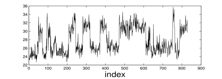
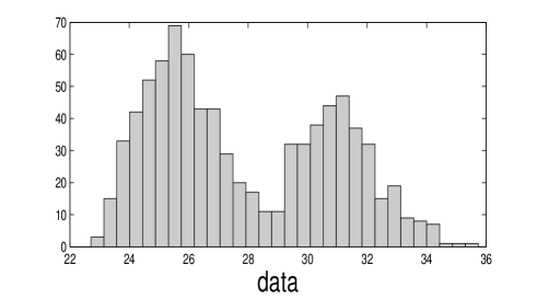
Figure 1: Every 30th observation from the data in Figure 5 is considered here.

Algorithm 2 reports our ABC-MCMC procedure. The algorithm proposes simultaneously draws for ${\bm{\eta}}$ and $\delta$ with the purpose of retrospectively filtering-out the ${\bm{\eta}}$’s by retaining only those corresponding to sufficiently small $\delta$’s. Further, the algorithm is often able to “early-reject” proposed draws without having to generate ${\bm{z}}_{sim}$ due to our choice of a uniform kernel for $\rho(\cdot)$; i.e. we set

$$\rho({\bm{S}}_{n^{\prime}}({\bm{z}}_{sim}),{\bm{S}}_{n}({\bm{z}}))=K\left(\frac{|{\bm{S}}_{n^{\prime}}({\bm{z}}_{sim})-{\bm{S}}_{n}({\bm{z}})|}{\delta}\right)$$

where

$$K({\bm{w}})=I({\bm{w}}\colon\,{\bm{w}}^{T}\mathbf{A}{\bm{w}}<\pi^{-1}(\Gamma(d_{s}/2)d_{s}/2)^{2/d_{s}}|\mathbf{A}|^{1/d_{s}}).$$ (5)

The $\pi$ in (5) denotes the mathematical constant, $I(\cdot)$ is the indicator function and $\mathbf{A}$ is a user-defined $d_{s}\times d_{s}$ diagonal matrix of positive weights scaling the values of the entries in the vector of summary statistics. Notice that the quantity on the right hand side of the inequality in (5) is the unique value such that the volume of the region ${\bm{w}}^{T}\mathbf{A}{\bm{w}}$ equals 1. We refer to Fearnhead and Prangle (2012); Picchini (2014) for additional details. We can initially check whether to reject the proposed $({\bm{\eta}}^{\prime},\delta^{\prime})$ by evaluating a part of the traditional Metropolis-Hastings acceptance ratio; the one denoted as “ratio” in algorithm 2 below. When the draw $\omega\sim U(0,1)$ from the uniform distribution in step 2 is larger than this ratio we can immediately reject the proposed parameters regardless the value of $K(\cdot)\in\{0,1\}$ (which in fact does not need to be computed at this stage) and without having to simulate ${\bm{z}}_{sim}$. When $\omega$ is smaller or equal than “ratio” ${\bm{z}}_{sim}$ is produced and the usual Metropolis-Hastings procedure is resumed. This is extremely beneficial from the computational point of view, especially since ABC methods are usually performed at low acceptance rates. Another “early rejection” mechanism for ABC has been suggested in the “one-hit MCMC-ABC” algorithm by Lee and Andrieu (2012). Notice in step 1 of the algorithm the proposal mechanism for ${{\bm{\eta}}}$ and $\delta$ is written in a very general way: however in our experiments we assume the two quantities to be independent and therefore we could also write $u({{\bm{\eta}}},\delta|{{\bm{\eta}}}_{r},\delta_{r})=u_{1}({{\bm{\eta}}}|{{\bm{\eta}}}_{r})u_{2}(\delta|\delta_{r})$ with $u_{1}(\cdot)$ and $u_{2}(\cdot)$ the corresponding proposal distributions. For $u_{1}(\cdot)$ we employ an automatically tuned Metropolis random walk with Gaussian innovations Haario et al. (2001). Therefore in practice $u_{1}$ is used to simulate log-transformed parameters ${\bm{\eta}}=(\log\theta,\log\kappa,\log\gamma,\log\mu_{1},\log\mu_{2},\log\sigma_{1},\log\sigma_{2},\log\alpha)$. For $u_{2}$ we consider a (truncated) Gaussian Metropolis random walk on the support $(-\infty,\log\delta_{max}]$ where $\delta_{max}$ is initially set by the user and during the algorithm execution it gets automatically decreased until a user defined threshold $\delta_{minmax}$ is reached (see the update step in algorithm 2). In our experiments the update procedure for $\delta_{max}$ is executed every $g=3,000$ ABC-MCMC iterations using $m=99$, i.e. $\delta_{max}$ is assigned the 99th percentile from the last $g$ simulated values $\delta_{(l-1)g:lg-1}:=(\delta_{(l-1)g},\delta_{(l-1)g+1},...,\delta_{lg-1})$, for $l=1,2,...$, see also Lenormand et al. (2013). If the percentile is smaller than $\delta_{minmax}$ we set $\delta_{max}:=\delta_{minmax}$. This way the algorithm does not waste computational time for simulations corresponding to excessively large values of $\delta$. Of course the choice of $\delta_{max}$ and $\delta_{minmax}$ is applications specific and has to be a balanced compromise between exploration of the posterior surface (not too small $\delta_{max}$ nor $\delta_{minmax}$) and inferential accuracy (not too large $\delta_{max}$ and $\delta_{minmax}$).

0. Initialization: Compute ${\bm{S}}_{n}({\bm{z}})$. Fix $R$, $m$, $g$, $\delta_{minmax}<\delta_{max}$ and $\delta_{start}\leq\delta_{max}$. Simulate ${{\bm{\eta}}}_{start}\sim\pi({{\bm{\eta}}})$, ${{\bm{x}}}_{start}\sim\pi({{\bm{x}}}|{{\bm{\eta}}}_{start})$, and ${\bm{z}}_{start}\sim\pi({\bm{z}}|\tau({\bm{x}}_{start}),{\bm{\eta}}_{start})$. Set $r=0$, $({{\bm{\eta}}}_{0},\delta_{0})\equiv({{\bm{\eta}}}_{start},\delta_{start})$, and ${{\bm{S}}}_{n^{\prime}}({{\bm{z}}}_{sim,0})\equiv{{\bm{S}}}_{n^{\prime}}({{\bm{z}}}_{start})$.

At $(r+1)$th ABC-MCMC iteration:

1. generate $({\bm{\eta}}^{\prime},\delta^{\prime})\sim u({\bm{\eta}},\delta|{{\bm{\eta}}}_{r},\delta_{r})$ and update $\delta_{max}$ if appropriate (see $\star$ below);

2. generate $\omega\sim U(0,1)$;

if 

$$\omega>\frac{\pi({{\bm{\eta}}}^{\prime})\pi(\delta^{\prime})u({{\bm{\eta}}}_{r},\delta_{r}|{{\bm{\eta}}}^{\prime},\delta^{\prime})}{\pi({{\bm{\eta}}}_{r})\pi(\delta_{r})u({{\bm{\eta}}}^{\prime},\delta^{\prime}|{{\bm{\eta}}}_{r},\delta_{r})}\qquad(=\text{``ratio''})$$

 then

    $({{\bm{\eta}}}_{r+1},\delta_{r+1},{{\bm{S}}}_{n^{\prime}}({{\bm{z}}}_{sim,r+1})):=({{\bm{\eta}}}_{r},\delta_{r},{{\bm{S}}}_{n^{\prime}}({{\bm{z}}}_{sim,r}))$; $\triangleright$ (proposal early-rejected)

else generate ${{\bm{x}}}_{sim}\sim\pi({{\bm{x}}}|{{\bm{\eta}}}^{\prime})$ and ${{\bm{z}}}_{sim}\sim\pi({{\bm{z}}}|\tau({\bm{x}}_{sim}),{{\bm{\eta}}}^{\prime})$ conditionally on the ${{\bm{\eta}}}^{\prime}$ from step 1

    if $K(|{{\bm{S}}}_{n^{\prime}}({{\bm{z}}}_{sim})-{{\bm{S}}}_{n}({{\bm{z}}})|/\delta^{\prime})=0$ then

        $({{\bm{\eta}}}_{r+1},\delta_{r+1},{{\bm{S}}}_{n^{\prime}}({{\bm{z}}}_{sim,r+1})):=({{\bm{\eta}}}_{r},\delta_{r},{{\bm{S}}}_{n^{\prime}}({{\bm{z}}}_{sim,r}))$ $\triangleright$ (proposal rejected)

    else if $\omega\leq\mathrm{ratio}$ then

        $({{\bm{\eta}}}_{r+1},\delta_{r+1},{{\bm{S}}}_{n^{\prime}}({{\bm{z}}}_{sim,r+1})):=({{\bm{\eta}}}^{\prime},\delta^{\prime},{{\bm{S}}}_{n^{\prime}}({{\bm{z}}}_{sim}))$ $\triangleright$ (proposal accepted)

    else

        $({{\bm{\eta}}}_{r+1},\delta_{r+1},{{\bm{S}}}_{n^{\prime}}({{\bm{z}}}_{sim,r+1})):=({{\bm{\eta}}}_{r},\delta_{r},{{\bm{S}}}_{n^{\prime}}({{\bm{z}}}_{sim,r}))$ $\triangleright$ (proposal rejected)

    end if

end if

3. increment $r$ to $r+1$. If $r>R$ stop, else go to step 1.

^⋆ This is the update procedure for $\delta_{max}$:

When iteration $r$ is a multiple of a positive integer $g$, i.e. $r=l\cdot g$ for $l=1,2,...$ set $\delta_{max}$ as the $m$th percentile of $\delta_{(l-1)g:r-1}$. If $\delta_{max}<\delta_{minmax}$ set $\delta_{max}:=\delta_{minmax}$.

Algorithm 2 Early–Rejection ABC-MCMC

Note that whenever we write ${\bm{x}}_{sim}\sim\pi({\bm{x}}|{\bm{\eta}^{\prime}})$ it means that we are simulating the Markov process $\{X_{t}\}$ conditionally on some ${\bm{\eta}^{\prime}}$ using (3) and starting at $X_{0}=x_{0}$, where $x_{0}$ is a constant determined in section 6. Once ${\bm{x}}_{sim}$ is available we apply the $\tau(\cdot)$ transformation to obtain $\tau({\bm{x}}_{sim})$ and then add a realization of $\{U_{t}\}$ (generated using its own transition density and of course conditionally on ${\bm{\eta}^{\prime}}$). The result is a realization of what is synthetically denoted with ${{\bm{z}}}_{sim}\sim\pi({{\bm{z}}}|\tau({\bm{x}}_{sim}),{{\bm{\eta}}}^{\prime})$, that is a realization of process $\{Z_{t}\}$.

All trajectories are generated at times belonging to the subsample $\{t_{i_{1}},t_{i_{2}},...,t_{i_{n^{\prime}}}\}$, i.e. ${\bm{z}}_{sim}=(z_{sim,t_{i_{1}}},...,z_{sim,t_{i_{n^{\prime}}}})$ (and similarly for ${\bm{x}}_{sim}$) and the corresponding ${\bm{S}}_{n^{\prime}}({\bm{z}}_{sim})$ is then compared to the statistics for the full dataset ${\bm{S}}_{n}({\bm{z}})$. Also notice that conditional independence of observations is nowhere invoked in algorithm 2, which is therefore suitable for the diffusion model with error (1). Algorithm 2 produces $R$ draws $\{{\bm{\eta}}_{r},\delta_{r}\}_{r=1:R}$ from the augmented posterior $\pi({\bm{\eta}},\delta|\rho({\bm{S}}({\bm{z}}_{sim}),{\bm{S}}({\bm{z}}))\leq\delta)$ but we are only interested in the marginal posterior $\pi({\bm{\eta}}|\rho({\bm{S}}({\bm{z}}_{sim}),{\bm{S}}({\bm{z}}))\leq\delta)$: therefore once the algorithm run has been completed we filter-out draws for ${\bm{\eta}}$ which are not consistent with some suitable (small enough) threshold $\delta^{*}$. A strategy for “filtering” the output and determining $\delta^{*}$ is illustrated in section 5, see also Picchini (2014); Bortot et al. (2007).

5 Simulation study: a comparison with exact Bayesian inference

We have conducted a small-sample simulation study to compare results from our ABC-MCMC algorithm with exact Bayesian inference based on the particle MCMC methodology Andrieu et al. (2010) in form of a parallelised version proposed in Drovandi (2014).

Particle MCMC produces exact Bayesian inference whenever an unbiased estimate $\hat{p}({\bm{z}}|{\bm{\eta}})$ to the likelihood in (4) can be computed. This is possible for model (1) as explained in what follows. Note that conditionally on the latent state $\{\tau(X_{0})=\tau(x_{0}),\ldots,\tau(X_{{j}})=\tau(x_{{j}})\}$, the observation $(z_{0},\ldots,z_{{j}})$ is merely a translation of the measurement errors thus having density $p(z_{0},\ldots,z_{{j}}|\tau(x_{0}),\ldots,\tau(x_{{j}});{\bm{\eta}})$ equal to

$$\frac{1}{\gamma}\cdot\phi\left(\frac{z_{{0}}-\tau(x_{{0}})}{\gamma}\right)\times\prod_{i=1}^{j}\frac{1}{\gamma\sqrt{1-e^{-2\kappa\Delta_{i}}}}\cdot\phi\left(\frac{z_{i}-\tau(x_{i})-e^{-\kappa\Delta_{i}}(z_{{i-1}}-\tau(x_{{i-1}}))}{\gamma\sqrt{1-e^{-2\kappa\Delta_{i}}}}\right),$$

where $\Delta_{i}=t_{i}-t_{i-1}$ and where $\phi(\cdot)$ denotes the density of the standard Gaussian distribution. We obtain an approximation to $p(z_{0},...,z_{j}|{\bm{\eta}})$ via SMC by use of the bootstrap filter of Gordon et al. (1993), see also Doucet et al. (2001). Let $\{\tau(x_{i-1}^{l})\}$ denote the set of $N$ particles available at time $t_{i-1}$ before randomisation occur, and $\{\tau(\tilde{x}_{i-1}^{l})\}$ the resulting randomised particles which are used as a starting point to propagate particles forward to time $t_{i}$. Then

$$\hat{p}(z_{0},...,z_{j}|{\bm{\eta}})=\prod_{i=1}^{j}\hat{p}(z_{i}|z_{0},...,z_{i-1};{\bm{\eta}})=\prod_{i=1}^{j}\frac{1}{N}\sum_{l=1}^{N}w_{i}^{l}$$

with weights $w_{i}^{l}$ ($l=1,...,N$; $i=1,...,n$) given by

$$w_{i}^{l}=\frac{1}{\gamma\sqrt{1-e^{-2\kappa\Delta_{i}}}}\cdot\phi\left(\frac{z_{i}-\tau(x_{i}^{l})-e^{-\kappa\Delta_{i}}(z_{i-1}-\tau(\tilde{x}_{i-1}^{l}))}{\gamma\sqrt{1-e^{-2\kappa\Delta_{i}}}}\right).$$ (6)

Note that $w_{i}^{l}$ depend on $\tau(\tilde{x}_{i-1}^{l})$ which is the parent of $\tau(\tilde{x}_{i}^{l})$ in the genealogy of the $l$’th particle. Finally we can compute the (unbiased) likelihood approximation

$$\hat{p}({\bm{z}}|{\bm{\eta}}) =\hat{p}(z_{0}|{\bm{\eta}})\prod_{i=1}^{n}\hat{p}(z_{i}|z_{0},...,z_{i-1};{\bm{\eta}})$$

$$\text{where}\quad\hat{p}(z_{0}|{\bm{\eta}}) =\frac{\sum_{l=1}^{N}w_{0}^{l}}{N},\quad w_{0}^{l}=\frac{1}{\gamma}\cdot\phi\biggl{(}\frac{z_{0}-\tau(\tilde{x}_{0}^{l})}{\gamma}\biggr{)}.$$

The procedure above can be parallelised over $M$ machines/cores to obtain $M$ independent approximations of $p({\bm{z}}|{\bm{\eta}})$ for the running value of ${\bm{\eta}}$. The average of these approximations is a more precise (unbiased) estimate of the likelihood which can be used in the Metropolis-Hastings procedure to produce exact Bayesian inference for ${\bm{\eta}}$. Parallel computation improves the mixing of the resulting chain for particle MCMC, although only marginally for a small $M$. We used the parfor functionality from the Parallel Computing Toolbox for Matlab (release R2013a) with $M=4$ cores and $N=100$ particles for each core.

As mentioned in section 3, running an exact Bayesian algorithm based on SMC on a large dataset is extremely time consuming when considering a model such as (1). This would be the case with the sample size $n=24,842$ of the data in our application, section 6. Therefore we conduct a simulation study with artificial data of a much smaller size. As model parameters we used the parameters denoted with “true values” in Table 1. Setting the initial state to $x_{0}=-2.45$ we produced $n=355$ observations from model (1) at times $\{1,71,141,...,24781\}$. The simulated data (not reported) have switching structure resembling Figure 1. Please note that in this case we are not making use of subsampling as the $n=n^{\prime}=355$ data points are considered to be a full dataset. Therefore, ABC and exact Bayesian results are based on the same amount of data. A proper subsampling experiment is considered in section 6.

We employ the following uniform priors: $\log\theta\sim U(-7,-5.3),$ $\log\kappa\sim U(-1.5,0.3)$, $\log\gamma\sim U(-0.7,0.5)$, $\log\mu_{1}\sim U(3.1,3.3)$, $\log\mu_{2}\sim U(3.3,3.7)$, $\log\sigma_{1}\sim U(-2.5,1)$, $\log\sigma_{2}\sim U(-2.5,1)$, $\log\alpha\sim U(-1.5,-0.05)$. The ABC summary statistics comprise autocorrelation values at lags 2, 5, 10 and 15 together with the 15, 30, 45, 60, 75, 90th percentiles for both ${\bm{z}}$ and ${\bm{z}}_{sim}$. Hence, both ${\bm{S}}_{n}(\cdot)$ and ${\bm{S}}_{n^{\prime}}(\cdot)$ have length $d_{s}=10$. Algorithm 2 was run for $R=2\times 10^{6}$ iterations, with starting bandwidth $\delta_{start}=0.5$ and exponential prior on $\delta\sim Exp(0.2)$. The proposals for $\log\delta$ were generated via (truncated) Gaussian Metropolis random walk on the support $(-\infty,\log\delta_{max}]$ using steps having variance 0.2. We update the initial $\delta_{max}=0.8$ as described in section 4.1 and using $\delta_{minmax}=0.47$. The weight matrix $\mathbf{A}$ defining the uniform kernel (5) was set to $\mathrm{diag}(\mathbf{A})=[100,100,100,100,1,1,1,1,1,1]$. This assigns larger weights to the autocorrelations to compensate for their smaller values compared to the percentiles. Results were obtained in about 4.7 hrs on a Intel Core i7-2600 CPU 3.40 GhZ with 4 Gb RAM. We observed an acceptance rate in the range 0.3–1% during the simulations, which is a good compromise between statistical accuracy (the smaller $\delta$ the larger the rejection rate) and exploration of the posterior surface. We thinned the generated chain by retaining each 10th draw and then removed as burnin the first 30,000 draws, essentially disregarding draws corresponding to the update phase for $\delta_{max}$ and $\delta_{minmax}$, see Figure 2.

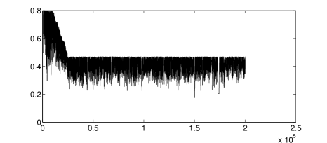
Figure 2: Thinned chain for $\delta$ for the simulated data problem.

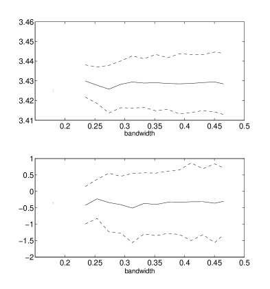
Figure 3: Marginal posterior means vs $\delta$ before filtering the ABC-MCMC output [$\pm 2$ SD] for $\log\mu_{2}$ (top) and $\log\sigma_{2}$ (bottom).

Finally by inspecting plots as in Figure 3 we “filtered” the remaining chain by studying the posterior means for varying values of $\delta$ and ultimately selected draws for ${\bm{\eta}}$ corresponding to $\delta$’s not exceeding $\delta^{*}=0.35$, where $\delta^{*}$ has been defined at the end of section 4.1. Note that this is possible as our ABC-MCMC algorithm produces chains for both ${\bm{\eta}}$ and $\delta$. Inferential results from the remaining 28,000 draws are compared to particle MCMC (exact Bayesian inference) in Table 1. The particle MCMC algorithm was run for $R=200,000$ iterations. Results were obtained in about 67 hrs, with an average acceptance rate of 10%. After removing the initial 25,000 draws (burn-in) we produced the exact (up to Monte Carlo sampling) inferential results given in Table 1.

Table 1: Posterior means and 95% posterior intervals from particle MCMC (lines without asterisks) and ABC-MCMC (lines with asterisks) when $n=355$.

	True values
$\log\theta$	$-5.914$	$-6.108$	$[-6.634,-5.700]$
		$-6.244^{*}$	$[-6.744,-5.738]$
$\log\kappa$	$-0.620$	$-0.811$	$[-1.473,0.206]$
		$-0.902^{*}$	$[-1.460,0.014]$
$\log\gamma$	0.061	0.072	$[-0.040,0.171]$
		$-0.002^{*}$	$[-0.233,0.219]$
$\log\mu_{1}$	3.24	3.24	$[3.24,3.25]$
		$3.25^{*}$	$[3.23,3.26]$
$\log\mu_{2}$	3.43	3.43	$[3.42,3.43]$
		$3.43^{*}$	$[3.42,3.44]$
$\log\sigma_{1}$	$-0.616$	$-0.401$	$[-0.803,-0.077]$
		$-1.586^{*}$	$[-2.359,-1.088]$
$\log\sigma_{2}$	$-0.472$	$-0.852$	$[-1.936,-0.190]$
		$-0.392^{*}$	$[-1.379,0.373]$
$\log\alpha$	$-0.622$	$-0.652$	$[-0.970,-0.426]$
		$-0.630^{*}$	$[-0.916,-0.423]$

Figure 4 reports the estimated marginal posterior densities from the particle MCMC and ABC-MCMC methods. The “static” features of the model represented by ${\bm{\psi}}=(\mu_{1},\mu_{2},\sigma_{1},\sigma_{2},\alpha)$ seem to be overall well captured by both inferential procedures. The modes $\mu_{1}$ and $\mu_{2}$ and the mixture parameter $\alpha$ can easily be identified, while the variance parameters $\gamma$, $\sigma_{1}$, and $\sigma_{2}$ are somewhat harder to identify and ABC appears to fail for $\sigma_{1}$ (this parameter is better estimated when using a larger sample size, see below). Regarding the correlation parameters $\theta$ and $\kappa$, less information is available from the data and the posteriors do not dominate strongly over the prior. In particular, $\kappa$ can hardly be identified, which is likely due to the “thinning” of the data leaving little information on the short scale correlation (recall that $\kappa$ is the correlation parameter of the measurement error process). This is confirmed by further results below as well as in section 6, where several levels of subsampling are considered and the identification of $\kappa$ improves for a smaller $q$. We conclude that in this preliminary analysis ABC has shown an overall satisfactory performance. We now produce further results using a larger sample size $n=n^{\prime}=1,380$ while maintaining all other settings unchanged to obtain the following posterior inference (means and 95% posterior intervals for each parameter), $\log\theta$: $-6.275$ $[-6.950,-5.624]$, $\log\kappa$: $-0.538$ $[-1.407,0.219]$, $\log\gamma$: $-0.027$ $[-0.540,0.263]$, $\log\mu_{1}$: $3.24$ $[3.22,3.25]$, $\log\mu_{2}$: $3.43$ $[3.41,3.45]$, $\log\sigma_{1}$: $-1.017$ $[-2.362,0.083]$, $\log\sigma_{2}$: $-0.854$ $[-2.240,0.419]$, $\log\alpha$: $-0.697$ $[-1.159,-0.396]$. Clearly the estimation of $\kappa$ and $\sigma_{1}$ has improved. Unfortunately we cannot perform a comparison with particle MCMC when $n=1,380$ as this would require about 260 hrs of computation. Finally we check for possible improvements when using $n=1,380$ together with a larger set of percentiles in our vector of summary statistics (in addition to the usual autocorrelation values): we consider nine percentiles instead of six, i.e. the 10th, 20th,…,90th empirical percentiles. We select $\delta^{*}=0.4$ and obtain the following posterior inference: $\log\theta$: $-6.247$ $[-6.734,-5.706]$, $\log\kappa$: $-0.534$ $[-1.448,0.220]$, $\log\gamma$: $0.003$ $[-0.371,0.225]$, $\log\mu_{1}$: $3.24$ $[3.22,3.25]$, $\log\mu_{2}$: $3.43$ $[3.41,3.45]$, $\log\sigma_{1}$: $-1.025$ $[-2.419,0.095]$, $\log\sigma_{2}$: $-0.877$ $[-2.402,0.321]$, $\log\alpha$: $-0.627$ $[-0.959,-0.398]$. No striking difference emerges in comparison with the previous analysis, therefore we prefer to use only six percentiles, as the larger the size $d_{s}$ of $S(\cdot)$, when compared to $\mathrm{dim}(\theta)$, the larger the Monte Carlo error (Lemma 1 in (Fearnhead and Prangle, 2012)).

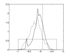
(a) $\log\theta$

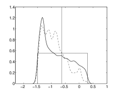
(b) $\log\kappa$

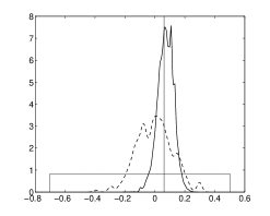
(c) $\log\gamma$

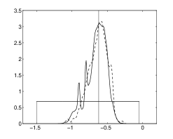
(d) $\log\alpha$

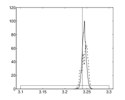
(e) $\log\mu_{1}$

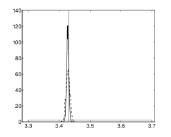
(f) $\log\mu_{2}$

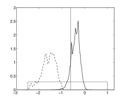
(g) $\log\sigma_{1}$

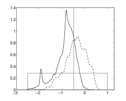
(h) $\log\sigma_{2}$

Figure 4: Inference from simulated data when $n=355$: posterior marginal densities (by kernel smoothing approximation) for ABC-MCMC (dashed lines), particle MCMC (solid lines) and uniform priors. Vertical lines mark true parameter values. See the main text for further results.

A striking difference between ABC and particle MCMC lies in the computational cost: for the case $n=355$ a cycle of 1,000 iterations of particle MCMC is completed in 1,210 sec whereas for ABC-MCMC it requires only 6.5 sec. This makes it difficult to overlook an approximate inferential method such as ABC-MCMC. Of course the price to be paid is the difficulty in tuning ABC algorithms and most importantly choose the summary statistics. The choice of kernel $K(\cdot)$ and tolerance $\delta$ is not particularly challenging. However particle MCMC methods require not so much tuning (once efficient proposal functions are constructed, and this is not an easy task in general) and return draws exactly from the posterior. Important examples of successful application of ABC are e.g. Barthelmé and Chopin (2014) using expectation-propagation and Toni et al. (2009) using SMC within ABC.

6 Application: A protein folding problem

Proteins are synthesized in the cell on ribosomes as linear, unstructured polymers that self-assemble into specific and functional three-dimensional structures. This self-assembly process, called protein folding, is the last and crucial step in the transformation of genetic information, encoded in DNA, into functional protein molecules. Because of its biological importance, the understanding of protein folding has received enormous interest both in experiments, theory and simulations (Wolynes et al., 2012). For reasons of simplification and tractability, the dynamics of a protein are often modelled as diffusions along a single reaction coordinate, that is one-dimensional diffusion models are considered to model a projection of the actual dynamics in high-dimensional space, see Socci et al. (1996); Das et al. (2006) and references therein. In our case study we consider the so-called L-reaction coordinate of the small Trp-zipper protein with $n=24,842$ observations taken at a sampling frequency of $\Delta^{-1}=$1/nsec. The high-dimensional dynamics of the protein were simulated from the Monte Carlo algorithm of Bottaro et al. (2012) using the PHAISTOS software package Boomsma et al. (2013). Alongside the L-reaction coordinate was computed. The sample path of the reaction coordinate, Figure 5, clearly reflects the random switching of the protein between the folded (lower mode) and unfolded (upper mode) state.

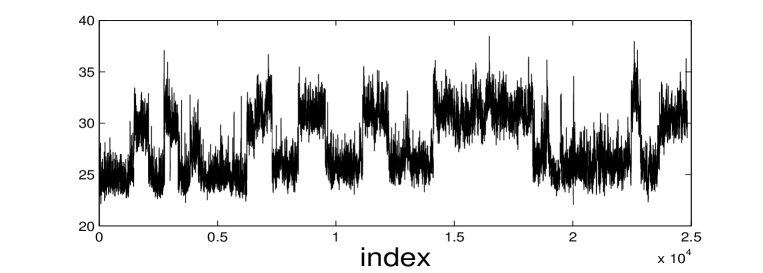
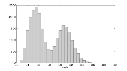
Figure 5: Sample path and sample histogram of the so-called $L$-projection of the small Trp-zipper protein. The distribution of the data reflects the two states of the protein.

In a preliminary analysis, Forman and Sørensen (2014) found that these data were not well fitted by any Markovian model, but that the diffusion observed with measurement error model (1) gave a good fit both on the short and on the long time scale.

To estimate the parameter ${\bm{\eta}}$ from the protein data we apply the ABC algorithm 2. The priors and the overall setup is the same as in the simulation study but this time we use subsampling in the simulations within algorithm 2. In fact we perform three studies where a different value for the subsample size $n^{\prime}$ (hence a different $q$) is considered in each case: in the first study trajectories are simulated in correspondence of every $q=30$’th observation of the full data, so that $n^{\prime}=829$ and the ${\bm{x}}_{sim}$’s (and ${\bm{z}}_{sim}$’s) are simulated at times $\{t_{0},t_{30},t_{60},...,t_{n-30},t_{n}\}=\{1,31,61,...,24841\}$. Similarly in the other two studies we choose $q=15$ ($n^{\prime}=1,657$) and $q=7$ ($n^{\prime}=3,549$) respectively, and corresponding time grids. The algorithm assumes the initial state for $\{X_{t}\}$ to be a known constant $x_{0}$. Since $U\approx 0$ we have $x_{0}\approx\tau^{-1}(z_{0})$. The initial observation $z_{0}=23.248$ corresponds to the empirical $0.0072$-quantile of the data. Hence, in the three studies we set $x_{0}=\Phi^{-1}(0.0072)=-2.45$.

We now start discussing the experiment with $n^{\prime}=829$. As anticipated in section 4.1, we take values of the autocorrelation function as summary statistics, namely the ones at lags $(60,300,600,1200,1800,2100)$ for observed data ${\bm{z}}$ and at lags $(2,10,20,40,60,70)$ for ${\bm{z}}_{sim}$. Additionally we use the 15th, 30th, 45th, 60th, 75th and 90th empirical percentiles of both observed and simulated data as summary statistics. Thus ${\bm{S}}_{n}(\cdot)$ and ${\bm{S}}_{n^{\prime}}(\cdot)$ have length $d_{s}=12$. Finally we set $\delta_{start}=0.7$, $\delta_{max}=0.9$, $\delta_{minmax}=0.65$. Algorithm 2 was run for $R=2\times 10^{6}$ iterations, thinning every 10th draw and obtaining an average acceptance rate of about 1%. The simulation was completed in about 6.3 hrs when $n^{\prime}=829$. Same as in section 5 we observed how the posterior means of the ABC output change for varying values of $\delta$ and decided to filter-out draws corresponding to $\delta>\delta^{*}=0.45$. Results from the remaining 16,000 draws are shown in Table 2 and Figure 6. Same as before parameters $\kappa$ and $\sigma_{1}$ are quite uncertain, while the other parameters appears to be well identified from the data. In particular, we expect $\kappa$ to be better identified when increasing the size of the subsample, and this is confirmed in the other two studies. When experimenting with $n^{\prime}=1,657$ and $n^{\prime}=3,549$ we keep the same simulation settings as detailed above, including the choice $\delta^{*}=0.45$, and in the first case results were returned in 12.5 hrs and in 27.5 hrs in the second case. Results are compared in Table 2 and Figure 6. As expected, for increasing $n^{\prime}$ we note a markedly different approximated posterior for $\log\kappa$, because such parameter enters the autocorrelation function for the Ornstein-Uhlenbeck model $\{U_{t}\}$ and therefore a different subsampling has an effect on the autocorrelation function, hence an effect on $\kappa$. It is reassuring not to spot serious differences in the inference for the remaining parameters (except for $\sigma_{1}$), this implying that the information explained by our model (1) and contained in our summary statistics is preserved for different levels of subsampling and that a “harder” subsampling ($q=30$) does not seem to have a major influence on overall results.

Table 2: Protein folding data experiment: posterior means from the filtered ABC-MCMC output and 95% posterior intervals for the cases $n^{\prime}=829$ (first line of each estimated parameter), $n^{\prime}=1657$ (second line) and $n^{\prime}=3549$ (third line).

	ABC inference
$\log\theta$	–6.448	[–6.646,–5.909]
	–6.421	[–6.899,–5.847]
	–6.438	[–6.863,–5.891]
$\log\kappa$	–0.649	[–1.054,0.246]
	–0.492	[–1.202,0.185]
	-0.996	[–1.468,–0.522]
$\log\gamma$	0.070	[–0.052,0.378]
	-0.055	[–0.491,0.279]
	0.005	[–0.385,0.310]
$\log\mu_{1}$	3.24	[3.23,3.26]
	3.23	[3.21,3.26]
	3.24	[3.21,3.26]
$\log\mu_{2}$	3.43	[3.42,3.45]
	3.42	[3.39,3.45]
	3.43	[3.38,3.45]
$\log\sigma_{1}$	–0.962	[–1.665,0.364]
	–1.044	[–2.276,0.601]
	–0.719	[–2.269,0.546]
$\log\sigma_{2}$	–0.418	[–0.862,0.765]
	0.039	[–2.074,0.957]
	0.006	[–1.752,0.864]
$\log\alpha$	–0.663	[ –0.766,–0.383]
	–0.741	[–0.996,–0.420]
	–0.725	[–1.188,–0.399]

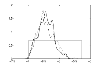
(a) $\log\theta$

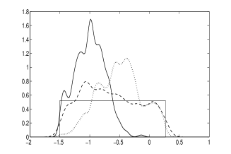
(b) $\log\kappa$

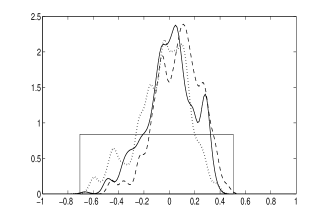
(c) $\log\gamma$

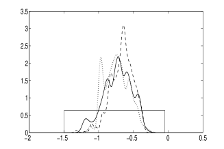
(d) $\log\alpha$

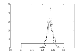
(e) $\log\mu_{1}$

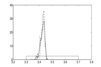
(f) $\log\mu_{2}$

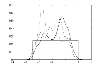
(g) $\log\sigma_{1}$

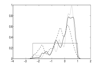
(h) $\log\sigma_{2}$

Figure 6: ABC inference from protein folding data: approximated marginal posteriors for subsamples having size $n^{\prime}=829$ (dashed line), $n^{\prime}=1657$ (dotted), $n^{\prime}=3549$ (solid) and uniform priors.

As a final informal check of our result we generated a time series of size $n=24,842$ from model (1) using parameters equal to the posterior means obtained for the case $n^{\prime}=829$. The sample path is compared to that of observed data in Figure 7. Although not perfect, the parameter estimates seem to capture the overall features in the data including timely switching between the two states. Corresponding trajectories for the case $n^{\prime}=3549$ do not result in noticeable differences and are thus not reported.

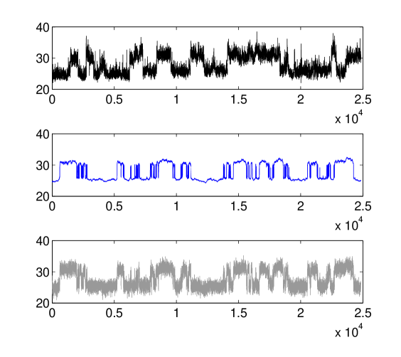
Figure 7: Comparison of protein folding data (top) with estimated processes $\tau(X_{t})$ (middle) and $Z_{t}$ (bottom) based on model 1 with parameters set to the estimated posterior means obtained for the case $n^{\prime}=829$.

7 Discussion

We have considered a complex stochastic dynamical model in form of a nonlinear diffusion observed with measurement error having a bimodal marginal structure with correlated error terms. The model has applications to a protein-folding problem where the data has size $n\approx 25,000$. Both the model and the size of data pose several problems both from a computational and a methodological point of view: (i) data analysed with the considered model are not conditionally independent given the latent state. This prevents the use of methods for state space models. (ii) The size of data prohibits the use of suitable but computer-intensive methods based on sequential Monte Carlo and likelihood-free Markov chain Monte Carlo (MCMC) algorithms. We proposed to conduct inference using approximated Bayesian computation (ABC) as a reasonable compromise between likelihood based inference and computational feasibility. An important feature of ABC is the ability to exploit the information carried by the data by means of summary statistics. We found that in our case ABC enables inference in a large data context by use of “subsampling”, that is while the entire dataset was used for inference, shorter trajectories, i.e. subsamples, were simulated within an ABC MCMC algorithm. Avoiding expensive simulations of latent trajectories having the same size as the available data is a major improvement in terms of time consumption and inferential results were encouraging. In fact the several levels of subsampling we investigated seem to affect only a small number of quantities in our model (specifically $\kappa$ and $\sigma_{1}$). This means that the speed we gain by simulating shorter trajectories does not translate in a significant loss of information, which is one of the advantages of using ABC, meaning that when available information is exploited via appropriate summaries (even if not sufficient statistics) satisfactory results can be obtained at a fraction of the cost corresponding to using the full data. Thus in the present case study the ABC method offered a valid alternative to exact but computationally expensive methodologies.

Other successful applications of subsampling can be found in Ahn et al. (2012); Korattikara et al. (2014) and it should be noted that it makes sense to consider subsampling for our specific application where dynamics follow a characteristic stationary pattern. In other applications, using subsampling may or may not be appropriate. Relevant and crucial comments on an early version of the present work have been raised in Christian P. Robert’s blog: one concern was the increased variability of the summary statistics when evaluated on a subsample. Given that we subsample dynamics having a fairly regular pattern, we expect that subsampling may lead to more variable results but not add any substantial bias. More in detail, both the empirical quantiles, empirical moments, and the empirical joint moments entering the summary statistics are M-estimators. Hence both the full sample and subsampled summary statistics are $\sqrt{n}$–consistent and asymptotically normal estimators of the true quantile/correlation-vector under suitable regularity conditions (see e.g. Newey (1990)) for large sample sizes and fixed subsampling level $q$. Under the true data generating measure the difference between the full data summary statistics and subsampled statistics generated independently hereof is thus approximately multivariate normal, with zero mean and a covariance matrix which could be derived from the asymptotic expansions of the estimators. This suggests that the inverse of the covariance for the difference would be an optimal weight in the distance measure and considered as matrix $\mathbf{A}$ into (5). However, the covariance matrix/optimal weight is in practice unknown as it depends on the true parameter. Ad hoc selections of this matrix are expected to produce asymptotically unbiased but suboptimal estimates. Note that subsampling in itself reduces efficiency as the asymptotic variance of the summary statistics is multiplied by a factor $q$. Giving a more formal account of the asymptotic properties of our estimators is technical and beyond the scope of the present paper.

Funding

Umberto Picchini and Julie Forman research is partly funded by a grant from the Swedish Research Council (VR grant 2013-5167).

References

- Ahn et al. (2012) S. Ahn, A. Korattikara, and M. Welling. Bayesian posterior sampling via stochastic gradient Fisher scoring. In John Langford and Joelle Pineau, editors, Proceedings of the 29th International Conference on Machine Learning, pages 1591–1598, 2012. arXiv:1206.6380.
- Aït-Sahalia (1996) Y. Aït-Sahalia. Testing continuous-time models of the spot interest rate. The Review of Financial Studies, 9:385–426, 1996.
- Andrieu et al. (2010) C. Andrieu, A. Doucet, and R. Holenstein. Particle Markov chain Monte Carlo methods (with discussion). Journal of the Royal Statistical Society: Series B, 72(3):269–342, 2010.
- Azencott et al. (2013) R. Azencott, B. Arjun, J. Ankita, and I. Timofeyev. Sub-sampling and parameter estimation for multiscale dynamics. Communications in Mathematical Sciences, 11:939–970, 2013.
- Barthelmé and Chopin (2014) S. Barthelmé and N. Chopin. Expectation propagation for likelihood-free inference. Journal of the American Statistical Association, 109(505):315–333, 2014.
- Beaumont (2010) M.A. Beaumont. Approximate Bayesian Computation in evolution and ecology. Annual Review of Ecology, Evolution, and Systematics, 41:379–406, 2010.
- Best and Hummer (2010) R. B. Best and G. Hummer. Coordinate-dependent diffusion in protein folding. PNAS, 107:1088–1093, 2010.
- Bezanson et al. (2012) J. Bezanson, S. Karpinskiy, V. B. Shah, and A. Edelman. Julia: A fast dynamic language for technical computing. arXiv:1209.5145v1, 2012.
- Boomsma et al. (2013) W. Boomsma et al. PHAISTOS: A framework for Markov chain Monte Carlo simulation and inference of protein structure. Journal of Computational Chemistry, 34(19):1697–1705, 2013.
- Bortot et al. (2007) P. Bortot, S.G. Coles, and S. Sisson. Inference for stereological extremes. Journal of the American Statistical Association, 102(477):84–92, 2007.
- Bottaro et al. (2012) S. Bottaro, W. E. Boomsma, K. Johansson, C. Andreetta, T. Hamelryck, and J. Ferkinghoff-Borg. Subtle Monte Carlo updates in dense molecular systems. Journal of Chemical Theory and Computation, 8:695–702, 2012.
- Bretó et al. (2009) C. Bretó, D. He, E. L. Ionides, and A. A. King. Time series analysis via mechanistic models. The Annals of Applied Statistics, 3(1):319–348, 2009.
- Crommelin and Vanden-Eijnden (2011) D. Crommelin and E. Vanden-Eijnden. Diffusion estimation from multiscale data by operator eigenpairs. SIAM Multiscale Modeling and Simulation, 9:1588–1623, 2011.
- Das et al. (2006) P. Das, M. Moll, H. Stamati, L. E. Kavraki, and C. Clementi. Low-dimensional, free-energy landscapes of protein-folding reactions by nonlinear dimensionality reduction. PNAS, 103:9885–9890, 2006.
- Doucet et al. (2001) A. Doucet, N. De Freitas, and N. Gordon. Sequential Monte Carlo methods in practice. Springer New York, 2001.
- Drovandi (2014) C. Drovandi. Pseudo-marginal algorithms with multiple CPUs. Queensland University of Technology, available at http://eprints.qut.edu.au/61505/, 2014.
- Fearnhead and Prangle (2012) P. Fearnhead and D. Prangle. Constructing summary statistics for approximate Bayesian computation: semi-automatic approximate Bayesian computation (with discussion). Journal of the Royal Statistical Society series B, 74:419–474, 2012.
- Forman and Sørensen (2014) J. L. Forman and M. Sørensen. A transformation approach to modelling multi-modal diffusions. Journal of Statistical Planning and Inference, 146:56–69, 2014.
- Girolami et al. (2013) M. Girolami, A. M. Lyne, H. Strathmann, D. Simpson, and Y. Atchade. Playing Russian roulette with intractable likelihoods. 2013. arXiv:1306.4032.
- Golightly and Wilkinson (2011) A. Golightly and D. J. Wilkinson. Bayesian parameter inference for stochastic biochemical network models using particle Markov chain Monte Carlo. Interface Focus, 1(6):807–820, 2011.
- Gordon et al. (1993) N. J. Gordon, D. J. Salmond, and A. F. M. Smith. Novel approach to nonlinear/non-Gaussian Bayesian state estimation. IEE PROCEEDINGS-F, 140(2):107–113, 1993.
- Haario et al. (2001) H. Haario, E. Saksman, and J. Tamminen. An adaptive Metropolis algorithm. Bernoulli, 7(2):223–242, 2001.
- Ionides et al. (2006) E. L. Ionides, C. Bretó, and A. A. King. Inference for nonlinear dynamical systems. Proceedings of the National Academy of Sciences, 103(49):18438–18443, 2006.
- Kloeden and Platen (1992) P. E. Kloeden and E. Platen. Numerical Solution of Stochastic Differential Equations. Springer, 1992.
- Korattikara et al. (2014) A. Korattikara, Y. Chen, and M. Welling. Austerity in MCMC land: cutting the Metropolis-Hastings budget. 2014. arXiv:1304.5299.
- Lee and Andrieu (2012) A. Lee and C. Andrieu. Discussion of “Constructing summary statistics for approximate Bayesian computation: semi-automatic approximate Bayesian computation”. Journal of the Royal Statistical Society series B, 74:419–474, 2012.
- Lenormand et al. (2013) M. Lenormand, F. Jabot, and G. Deffuant. Adaptive approximate Bayesian computation for complex models. Computational Statistics, 28(6):2777–2796, 2013.
- Marin et al. (2012) J. M. Marin, P. Pudlo, C. P. Robert, and R. Ryder. Approximate Bayesian computational methods. Statistics and Computing, 22(6):1167–1180, 2012.
- Murray (2013) L.M. Murray. Bayesian state-space modelling on high-performance hardware using LibBi. arXiv:1306.3277, 2013.
- Newey (1990) W.K. Newey. Semiparametric efficiency bounds. Journal of Applied Econometrics, 5(2):99–135, 1990.
- Pavliotis and Stuart (2007) G. A. Pavliotis and A. M. Stuart. Parameter estimation for multiscale diffusions. Journal of Statistical Physics, 127:741–781, 2007.
- Picchini (2013) U. Picchini. abc-sde: a Matlab toolbox for approximate Bayesian computation (ABC) in stochastic differential equation models, 2013. http://sourceforge.net/projects/abc-sde/.
- Picchini (2014) U. Picchini. Inference for SDE models via approximate Bayesian computation. Journal of Computational and Graphical Statistics, 23(4):1080–1100, 2014.
- Pokern et al. (2009) Y. Pokern, A. M. Stuart, and P. Wiberg. Parameter estimation for partially observed hypoelliptic diffusions. Journal of the Royal Statistical Society series B, 71:49–73, 2009.
- Pritchard et al. (1999) J. K. Pritchard, M. T. Seielstad, A. Perez-Lezaun, and M. W. Feldman. Population growth of human Y chromosomes: a study of Y chromosome microsatellites. Molecular Biology and Evolution, 16(12):1791–1798, 1999.
- Rößler (2010) A. Rößler. Runge-Kutta methods for the strong approximation of solutions of stochastic differential equations. SIAM Journal on Numerical Analysis, 48(3):922–952, 2010.
- Socci et al. (1996) N.D. Socci, J. N. Onuchic, and P. G. Wolynes. Diffusive dynamics of the reaction coordinate for protein folding funnels. Journal of Chemical Physics, 104:5860–5868, 1996.
- Toni et al. (2009) T. Toni, D. Welch, N. Strelkowa, A. Ipsen, and M. P. H. Stumpf. Approximate Bayesian computation scheme for parameter inference and model selection in dynamical systems. Journal of the Royal Society Interface, 6(31):187–202, 2009.
- Varin et al. (2011) C. Varin, N. Reid, and D. Firth. An overview of composite likelihood methods. Statistica Sinica, 21(1):5–42, 2011.
- Wilkinson (2012) D. J. Wilkinson. Stochastic Modelling for Systems Biology. CRC Press, second edition, 2012.
- Wolynes et al. (2012) P. G. Wolynes, W. A. Eaton, and A. R. Fersht. Chemical physics of protein folding. Proceedings of the National Academy of Sciences, 109(44):17770–17771, 2012.