Quantum correlations in the 1-D driven dissipative transverse field XY model.

Abstract

We study the non-equilibrium steady state (NESS) of a driven dissipative one-dimensional system near a critical point, and explore how the quantum correlations compare to the known critical behavior in the ground state. The model we study corresponds to a cavity array driven parametrically at a two photon resonance, equivalent in a rotating frame to a transverse field anisotropic XY model [C. E. Bardyn and A. Imamoğlu, Phys. Rev. Lett 109 253606 (2012)]. Depending on the sign of transverse field, the steady state of the open system can be either related to the ground state or to the maximum energy state. In both cases, many properties of the entanglement are similar to the ground state, although no critical behavior occurs. As one varies from the Ising limit to the isotropic XY limit, entanglement range grows. The isotropic limit of the NESS is however singular, with simultaneously diverging range and vanishing magnitude of entanglement. This singular limiting behavior is quite distinct from the ground state behavior, it can however be understood analytically within spin-wave theory.

I Introduction

A central feature of critical behavior in any non-mean-field phase-transition is the existence of a diverging correlation length Sachdev (2011); Kadanoff (2000). Such divergences explain why universal theories, controlled only by symmetries of the problem, apply in the vicinity of a critical point. They also lead to scaling behavior Kadanoff (2000) of correlation functions. More recently, it has been noted that measures of specifically quantum correlation, e.g. entanglement Nielsen and Chuang (2010), also show scaling behavior Osterloh et al. (2002); Osborne and Nielsen (2002); Vidal et al. (2003); Amico et al. (2008). Entanglement is one of the characteristic traits of quantum mechanics Nielsen and Chuang (2010) and is of practical significance as it captures quantum correlations which can be a resource for quantum cryptography, quantum teleportation, and dense coding Horodecki et al. (2009). Despite the diverging correlation length at critical points, entanglement generally has a finite range Osterloh et al. (2002); Osborne and Nielsen (2002); Amico et al. (2008), critical scaling is instead seen in the magnitude of the entanglement.

In a dissipative system, coupling to an external environment Breuer and Petruccione (2002) leads to dephasing, and consequent degradation of quantum correlations, ultimately reducing the system to a classical description Zurek (2003); Lo Franco et al. (2013). Nonetheless, in a coherently driven dissipative system, i.e. pumped by an external coherent drive, non-trivial steady states can be found Dimer et al. (2007); Hartmann (2010); Baumann et al. (2010); Nagy et al. (2010); Diehl et al. (2010); Ferretti et al. (2010); Lee et al. (2011); Marcos et al. (2012); Murch et al. (2012); Lee et al. (2012); Grujic et al. (2012); Dalla Torre et al. (2012, 2013); Le Boité et al. (2013); Jin et al. (2013); Lee et al. (2013); Genway et al. (2013); Hu et al. (2013). In an extended interacting driven dissipative system, such as an array of coupled nonlinear cavities as discussed below, this enables non-local quantum correlations to exist in the non-equilibrium steady state. Such systems allow one to study quantum correlations out of equilibrium, and to study whether dissipation has particular significance for distinctively quantum correlations such as entanglement.

The aim of this paper is to explore the range and scaling of quantum correlations in the non-equilibrium-steady-state (NESS) near to a critical point of the corresponding equilibrium system. A natural system in which to address such questions is an array of coupled cavities Hartmann et al. (2006); Greentree et al. (2006); Angelakis et al. (2007); Hartmann et al. (2008); Schmidt and Koch (2013). Such systems allow for tunable coupling and nonlinearity, and inevitably have dissipation, as light escapes from the cavities. Recently Bardyn and Imamoglu (2012) have shown that such systems can in certain limits map to dissipative spin chain models, as explained below. Their proposed configuration allows tuning of both the anisotropy of the spin-spin coupling, and of a transverse field. We study the non-equilibrium steady state, i.e. the long time behavior, in the presence of dissipation. Within this scenario, we determine the dependence of quantum correlations on both of these parameters, exploring the range from the transverse field Ising model to the transverse field XY model.

The transverse field Ising model is a paradigmatic example of quantum critical behavior Sachdev (2011), and so the scaling of entanglement in the equilibrium Ising model (or anisotropic XY model) was one of the first examples studied Osterloh et al. (2002); Osborne and Nielsen (2002); Vidal et al. (2003). As noted above, while the magnitude of entanglement shows critical scaling, the range over which non-zero entanglement exists does not Osterloh et al. (2002); Osborne and Nielsen (2002). This finite range behavior persists for all models in the Ising universality class Osborne and Nielsen (2002); Maziero et al. (2010); Štelmachovič Peter and Bužek Vladimír (2004). Following these early studies, there have been many subsequent explorations of critical entanglement, including the spin-boson system Le Hur (2008) which can be viewed as a phase transition of a dissipative quantum system. For a review, see Ref. Amico et al. (2008).

A major difficulty in understanding a many body quantum system is the exponential growth of Hilbert space dimension with the system size. One method to overcome this difficulty is to use a matrix product state (MPS) approach Vidal (2003, 2004). Such methods make use of the fact that many physically relevant states have entanglement which is either constant or grows at most polynomially with system size Zurek (2003); an MPS can efficiently represent such a state. The MPS representation of a state is the concept underlying the Density Matrix Renormalization Group (DMRG) White (1992, 1993) approach. While the DMRG was originally used as a method to determine ground states of interacting systems, it was later extended to study dynamics Cazalilla and Marston (2002); White and Feiguin (2004); Daley et al. (2004); Micheli et al. (2004); Clark and Jaksch (2004); Cai and Barthel (2013), by an approach known as time evolving block decimation (TEBD). All these approaches ultimately rely on the fact that an efficient MPS representation of the relevant states of the system exists, for a discussion of this see e.g. Ref. Schollwöck (2011). These approaches have also been extended to open systems (mixed states), by introducing matrix product operators (MPO) Zwolak and Vidal (2004); Orús and Vidal (2008); Prosen and Žnidarič (2009). This allows one to efficiently time evolve the density matrix equations of motion for one dimensional open systems, and thus find the non-equilibrium steady state.

The remainder of this paper is organized as follows. Section II reviews the basis of our calculations. In particular, sections II.1,II.2 introduce the effective Hamiltonian we study and its coupling to an external environment; section II.3 reviews the measures of quantum correlations we calculate; section II.4 outlines the MPO method we use to find the steady state. Section III then presents the results of our numerical calculation. After reviewing the nature of the steady state in section III.1, and comparing these results to the mean-field theory of our model in section  III.2, sections III.3,III.4,III.5 discuss the dependence of quantum correlations on each of the model parameters in turn. Finally, section IV discusses analytic calculations which can reproduce the behavior seen for weak driving. In section V we summarize our findings.

II Driven-dissipative model and observables

II.1 Effective Hamiltonian

Figure 1: (Color online) Cartoon illustrating coupled cavity array with hopping $J$, two-cavity pumping $\Omega$ and loss rate $\kappa$.

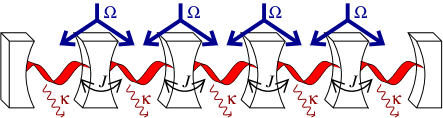
We consider a coupled cavity array realization of the transverse field anisotropic XY model, as introduced in Ref. Bardyn and Imamoglu (2012). For completeness, we briefly summarize the nature of such a model here. As illustrated in Fig. 1 the model consists of a 1-D array of optical cavities, supporting photon modes, described by bosonic operators $c_{j}$ with hopping amplitude $J$ between the cavities so that $H=\sum h_{j}-J\sum_{j}[c^{\dagger}_{j}c_{j+1}+\text{H.c.}]$. The on-site Hamiltonian, $h_{j}=\omega_{c}c^{\dagger}_{j}c_{j}+Uc^{\dagger}_{j}c^{\dagger}_{j}c_{j}c_{j}$, incorporates an optical nonlinearity $U$. Physically this can be induced by coupling each cavity to a saturable optical absorber Hartmann et al. (2006, 2008); Le Boité et al. (2013).

In addition to these elements, which would lead to a Bose-Hubbard model Fisher et al. (1989), we include a two-photon driving term as proposed in Ref. Bardyn and Imamoglu (2012). Specifically, we consider a drive $\Omega\cos(2\omega_{p}t)$ near two-photon resonance, i.e. $\omega_{p}\simeq\omega_{c}$, and we work in the limit of strong optical nonlinearity. In this limit, the problem simplifies, as one may truncate each site to occupations $0$ or $1$. Furthermore, this implies that the two-photon pump is only resonant for the creation of pairs of photons on adjacent cavities. When restricted to the $0,1$ occupation subspace, one may replace each cavity mode with a spin $1/2$, i.e. replace bosonic operators by Pauli matrices $(c_{j},c^{\dagger}_{j})\to(\sigma^{-}_{j},\sigma^{+}_{j})$. Here $\sigma^{\pm}_{j}=(\sigma^{x}_{j}\pm i\sigma^{y}_{j})/2$ in terms of regular Pauli matrices. In this notation, the Hamiltonian becomes:

$$\hat{H}_{0}=\sum_{j}\frac{\omega_{c}}{2}\sigma_{j}^{z}-J\sum_{j}\left(\sigma^{+}_{j}\sigma^{-}_{j+1}+\sigma^{-}_{j}\sigma^{+}_{j+1}\right)\\ -\Omega\sum_{j}\left(\sigma^{+}_{j}\sigma^{+}_{j+1}e^{-2i\omega_{p}t}+\sigma^{-}_{j}\sigma^{-}_{j+1}e^{2i\omega_{p}t}\right).$$ (1)

The explicit time dependence appearing here can be removed by a transformation to a rotating frame. In such a frame the Hamiltonian is given by:

$$\hat{H}=-J\sum_{j}\left[g\sigma_{j}^{z}+(\sigma_{j}^{+}\sigma_{j+1}^{-}+\sigma_{j+1}^{+}\sigma_{j}^{-})\right.\\ \left.+\Delta(\sigma_{j}^{+}\sigma_{j+1}^{+}+\sigma_{j+1}^{-}\sigma_{j}^{-})\right],$$ (2)

where we have introduced dimensionless parameters $g=(\omega_{p}-\omega_{c})/2J$ and $\Delta=\Omega/J$. This can also be written in the canonical form of the Ising model Mattis (2006):

$$\hat{H}=-J\sum_{j}\left[g\sigma_{j}^{z}+\frac{1+\Delta}{2}\sigma_{j}^{x}\sigma_{j+1}^{x}+\frac{1-\Delta}{2}\sigma_{j}^{y}\sigma_{j+1}^{y}\right].$$ (3)

The parameter $\Delta$ describes the anisotropy of the interaction: $\Delta=0$ corresponds to the isotropic $XY$ model, $\Delta=1$ to the Ising model. For $0<|\Delta|\leq 1$ the Hamiltonian is in the Ising universality class. In the ground state, changing the transverse field $g$ will induce a quantum phase transition Sachdev (2011) at $|g|=1$, between a phase with $\langle\sigma_{x}\rangle\neq 0$ for $|g|<1$, and a phase with vanishing $\langle\sigma_{x}\rangle$ for $|g|>1$.

II.2 Dissipation

In addition to the terms described so far, each cavity is also assumed to couple to a continuum of radiation modes describing irreversible loss into the environment Breuer and Petruccione (2002). At optical cavity and pump frequencies, one may eliminate such modes via the Born-Markov approximation Scully and Zubairy (1997); Breuer and Petruccione (2002), producing the master equation:

$$\frac{d}{dt}\rho=-i[\hat{H},\rho]+\kappa\sum_{j}[2\sigma_{j}^{-}{\rho}\sigma_{j}^{+}-\sigma_{j}^{+}\sigma_{j}^{-}\rho-\rho\sigma_{j}^{+}\sigma_{j}^{-}].$$ (4)

The dissipation described in Eq. (4) corresponds to independent incoherent loss from each cavity. In the spin language, this corresponds to a process that flips the spin from up to down. Such dissipation corresponds to a zero temperature bath, this is appropriate when considering optical frequency systems as the characteristic energy scales are much larger than temperature. In the following we introduce the dimensionless $\tilde{\kappa}=\kappa/J$, and consider the steady state of the system as a function of the parameters $(g,\Delta,\tilde{\kappa})$. In the remainder of the manuscript all energies are thus given in units of $J$.

It is important to note that the form of Eq. (4) can only follow from an originally time-dependent, i.e. pumped system. For a time-independent system coupled to an external bath, a correct treatment of the bath Cresser (1992) must lead to a Master equation which drives the system toward its thermal state. Such behavior is clearly required to be consistent with equilibrium statistical mechanics. The same is not however true of a time dependent Hamiltonian — in the rotating frame, coupling to the bath need not satisfy detailed balance due to the “extra” time dependence induced by the pump frequency Joshi et al. (2013). The crossover between these limits as one varies $\omega_{c},\omega_{p}$ while keeping $g$ constant is an interesting question for future work.

II.3 Measures of quantum correlations

To quantify the quantum correlations between different sites requires some care, since a given pair of sites will in general be entangled both with other sites and with the external environment. As such, it is important to use a measure of the quantum correlation between a specific pair of sites. The measure of pairwise entanglement we will use will be negativity, $\mathcal{N}$ defined as:

$$\mathcal{N}=\text{max}(0,\sum_{i}^{4}|\lambda_{i}|-1),$$ (5)

where $\lambda_{i}$ are the eigenvalues of the partially transposed two-qubit density matrix $\rho_{AB}^{T_{B}}$ Nielsen and Chuang (2010), where $T_{B}$ indicates transpose for system $B$. According to the Peres-Horodecki criterion Peres (1996); Horodecki et al. (1996) a (mixed) state of a bipartite system is separable if the negativity is zero. For any separable state, the density matrix would remain positive under a partial transpose. In an entangled state a partial transpose may produce a non-positive density matrix Lupo et al. (2005). The negativity as defined in Eq. (5) is a measure of whether the partial transpose produces negative eigenvalues. A non-zero value of negativity serves both as a necessary and sufficient condition for the inseparability of a general two qubit state Peres (1996); Horodecki et al. (1996).

For pure states entanglement is a sufficient measure of quantum correlations and quantifies the ability of a state to act as a resource for quantum computational speed-up Josza and Linden (2003). For mixed states separability (vanishing entanglement) does not in general imply classicality Ollivier and Zurek (2001); Henderson and Vedral (2001); Modi et al. (2012) — computational speed-up for mixed state quantum computing can occur without entanglement Knill and Laflamme (1998). Such speed-up has been attributed to the presence of non-zero quantum discord Ollivier and Zurek (2001); Henderson and Vedral (2001); Modi et al. (2012); Knill and Laflamme (1998); Dakić et al. (2012), $\mathcal{D}$ defined Modi et al. (2012) as follows: Consider a bipartite system AB in a state $\rho$, and a local measurement performed on subsystem B with its result ignored. Such a measurement will cause a disturbance of subsystem $A$ for almost all states. There is however a class, $\Omega$, of states that is unchanged by such a measurement. For such states $\chi\in\Omega$, known as “classical-quantum” states, one may write: $\chi=\sum_{i}p_{i}\rho_{Ai}\otimes|i\rangle_{B}{}_{B}\langle i|$, where $p_{i}$ is a probability distribution, $\rho_{Ai}$ is the marginal density matrix of A, and the states $|i\rangle_{B}$ form an orthonormal set. Geometric discord $\mathcal{D}$ is the distance between the state $\rho$ and the closest classical-quantum state $\chi\in\Omega$. Explicitly, for an arbitrary mixed state $\rho$ of a $d\otimes d$ quantum system it is $\mathcal{D}(\rho)=\frac{d}{d-1}\text{min}_{\chi\in\Omega}||\rho-\chi||^{2}$, where $||M||=\sqrt{\sum_{i}m_{i}^{2}}$ is the Hilbert-Schmidt norm of the operator $M$ with eigenvalues $m_{i}$.

In the specific case of two-level systems (qubits), a closed form for $\mathcal{D}$ exists Modi et al. (2012); Dakić et al. (2010) Writing the state of two qubits as:

$$\rho=\frac{1}{4}\sum_{i,j=0}^{3}R_{ij}\sigma_{i}\otimes\sigma_{j},\qquad\mathbf{R}=\left(\begin{array}[]{cc}1&\mathbf{y}^{T}\\ \mathbf{x}&\mathbf{t}\end{array}\right)$$ (6)

where $\sigma^{0,1,2,3}_{j}=\left\{\mathbbm{1}_{j},\sigma^{x}_{j},\sigma^{y}_{j},\sigma^{z}_{j}\right\}$, and $\mathbf{R}$ is given in block structure above, one may then construct the $3\times 3$ matrix $S=(1/4)(\mathbf{x}\mathbf{x}^{T}+\mathbf{t}\mathbf{t}^{T})$ from which

$$\mathcal{D}=2\text{Tr}[S]-2\lambda_{\text{max}}(S),$$ (7)

where $\lambda_{\text{max}}(S)$ is the largest eigenvalue of the matrix S.

II.4 Matrix product state evolution

As noted above, to find the non-equilibrium steady state, we time evolve Eq. (4) using a matrix product operator approach Zwolak and Vidal (2004); Orús and Vidal (2008); Prosen and Žnidarič (2009). We here briefly summarize the method used in our calculation. Further details of our specific implementation can be found in Ref. Nissen (2013).

Our problem requires time-evolving the density matrix of a chain of $N$ two-level systems. This density matrix may be written in the form:

$$\rho=\sum_{\{i_{1},i_{2},\ldots,i_{N}\}}c_{i_{1},i_{2},\ldots,i_{N}}\bigotimes_{j=1}^{N}\sigma_{j}^{i_{j}}$$ (8)

with $\sigma^{0,1,2,3}_{j}$ as given earlier forming a basis for the density matrix on each site. The central point of the MPO approach is to write the coefficients $c_{i_{1},i_{2},\ldots,i_{N}}$ in terms of matrices $\Gamma^{[j]i_{j}}$ and vectors $\lambda^{[j]}$ as follows:

$$c_{i_{1},i_{2},\ldots i_{N}}=\sum_{\{\alpha_{j}\}}\Gamma_{1,\alpha_{1}}^{[1]i_{1}}\lambda_{\alpha_{1}}^{[1]}\Gamma_{\alpha_{1},\alpha_{2}}^{[2]i_{2}}\ldots\\ \Gamma_{\alpha_{j-2},\alpha_{j-1}}^{[j-1]i_{j-1}}\lambda_{\alpha_{j-1}}^{[j-1]}\Gamma_{\alpha_{j-1},\alpha_{j}}^{[j]i_{j}}\ldots\Gamma_{\alpha_{N-2},\alpha_{N-1}}^{[N-1]i_{N-1}}\lambda_{\alpha_{N-1}}^{[N-1]}\Gamma_{\alpha_{N-1},1}^{[N]i_{N}}.$$

The matrix $\Gamma^{[j]i_{j}}$, corresponding to basis component $i_{j}$ on site $j$, is a $\chi_{j-1}\times\chi_{j}$ matrix, and $\lambda^{[j]}$ is a set of $\chi_{j}$ coefficients associated with the bond between site $j$ and site $j+1$. Here $\chi_{j}$ is the (integer) bond dimension of the matrix associated with bond $j$. If all $\chi_{j}=1$ then one has entirely separable density matrix, i.e. $\rho=\bigotimes\rho_{j}$, equivalent to a mean-field approximation. If $\chi_{j}$ are sufficiently large, any state can be written in the above form — the required size for our two-level-system density matrix is $\chi_{j}=\text{min}(4^{j},4^{N-j})$. To efficiently simulate such a system we restrict $\chi_{j}<\chi_{\text{max}}$. For a fixed $\chi_{\text{max}}$, the size of computation scales linearly with chain length. Despite this, the representation is able to accurately describe the full quantum dynamics in many problems.

To time-evolve the state, we follow the algorithm described in Ref. Vidal (2004); Orús and Vidal (2008). The Master equation may be written in a superoperator form, with the density matrix as a vector $\rho\to|\rho\rangle$, so that $\partial_{t}|\rho\rangle=M|\rho\rangle$. The superoperator $M$ can be decomposed as $M=\sum_{j}M^{\text{pair}}_{j,j+1}$, with the one-site operations split between the appropriate pair operators. Evolution by a time step $\delta t$ corresponds to propagating the coefficients $\Gamma^{[j]i_{j}},\lambda^{[j]}$ under the operator $\exp(M^{\text{pair}}_{j,j+1}\delta t)$. This is done by converting the MPO representation for a given pair of sites into its explicit form, evolving the pair, and then performing a singular value decomposition (SVD) Nielsen and Chuang (2010) to return the final form to MPO representation. The rank $\chi_{j}$ after such an update will generally have increased, but can be restored to $\chi_{j}\leq\chi_{\text{max}}$ by keeping only the largest $\chi_{\text{max}}$ singular values in the SVD.

To extend from a single pair to many, the overall superoperator $M$ can be divided into parts on odd and even sites $j$ and, using the Suzuki-Trotter expansion $e^{M\delta t}=e^{M^{\text{odd}}\delta t/2}e^{M^{\text{even}}\delta t}e^{M^{\text{odd}}\delta t/2}+\mathcal{O}(\delta t^{3})$. Since $M^{\text{odd}}$ involves a sum of pair operations which each mutually commute, all the updates in $M^{\text{odd}}$ can be performed in parallel. The same applies to $M^{\text{even}}$.

Figure 2: (Color online) Negativity $\mathcal{N}$ vs transverse field $g$, comparing MPO numerical solution for $\chi_{\text{max}}=20$ (blue-solid) to exact diagonalization (red-dashed) for a four-site Ising model. Parameters (in units of $J$): $\Delta=1$, $\tilde{\kappa}=0.5$.

To demonstrate the accuracy of our implementation Nissen (2013), Fig. 2 shows a comparison between exact diagonalization of the four-site Master equation and the open system MPO code with $\chi_{\text{max}}=20$ showing close agreement. These results, as all results in our paper, are calculated for a chain with open boundary conditions. For longer chains, comparison with exact solutions is not feasible so we instead check for convergence of numerical results with matrix rank $\chi_{\text{max}}$. Efficient simulation depends on whether convergence is achieved for sufficiently small values of the matrix rank $\chi_{\text{max}}$. If correlation lengths diverge, such as at critical points, strong long-range correlations exist. In such cases convergence would only occur at large $\chi_{\text{max}}$ and and evolution becomes computationally expensive. In our system, we will see that the dissipation $\tilde{\kappa}$ suppresses such long range correlations; for small values of $\tilde{\kappa}$ the computational cost would increase, particularly near the equilibrium critical points $|g|=1$. It is important also to note that in this paper we are only concerned with convergence of the steady-state properties. If one is also interested in the short time dynamics, the required matrix rank may be much larger Hartmann et al. (2009), due to transient correlations arising before dissipation has time to act. In addition to convergence with matrix rank, we also find and check that properties near the middle of the chain converge with increasing chain length.

III Scaling of quantum correlations in Non-equilibrium steady states

III.1 Nature of the Non-Equilibrium Steady state

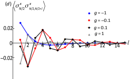
Before discussing the quantum correlations in the non-equilibrium steady state of Eq. (4), we first discuss the nature of the steady state itself. The dissipation term on its own would drive the system to a state with all spins pointing down. In the following we denote this state as the trivial empty state. In general (unless $\Delta=0$), this trivial state is not an eigenstate of the Hamiltonian so is not the steady state. An observable that gives a clear indication of the nature of the steady state is the correlation function $\langle\sigma^{x}_{j}\sigma^{x}_{j+l}\rangle$. This is plotted in Fig. 3 for $\Delta=1$, for sites near the center of the chain, hence avoiding edge effects.

Figure 3: (Color online) Panel (a) showing spin-spin correlations $\langle\sigma^{x}_{j}\sigma^{x}_{j+l}\rangle$ as a function of transverse field. The different lines correspond to different separations. Panel (b) showing decay of spin-spin correlations $\langle\sigma^{x}_{j}\sigma^{x}_{j+l}\rangle$ as a function of separation $l$ between the spin sites. Both panels plotted for the Ising limit ($\Delta=1$). It is clearly seen that the NESS exhibit FM and AFM ordering for negative and positive values of transverse field ($g=\pm 1$). Inset (panel (c)) shows short range incommensurate order for lower values of transverse field ($g=\pm 0.1$). The axes in the inset are same as in the main plot. Other parameters (in units of $J$): $\tilde{\kappa}=0.5$ and MPO calculation performed for $N=40$ site chain, with $\chi_{\text{max}}=20$.

As is clear from Fig. 3, in the NESS, the $x$ components of spin show (short range) ferromagnetic order for transverse fields around $g\simeq-1$ and antiferromagnetic order for fields around $g\simeq 1$. In comparison, in the ground state of the Ising model there are ferromagnetic correlations for $|g|<1$, regardless of the sign of $g$. As will be proven below, there is a direct relation between the NESS for positive and negative $g$, corresponding to a $\pi$ rotation around the $z$ axis on every second lattice site. This duality implies that if (short-range) ferromagnetic correlations are seen for a given $g$, anti-ferromagnetic correlations will exist for $g\to-g$. As well as this formal duality, we will also discuss next a more intuitive picture for the different behaviors at positive and negative $g$, a picture substantiated by analytic results of mean-field analysis given in Sec. III.2.

For large negative $g$, the ground state is compatible with the dissipation terms: both favor spins pointing in the $-z$ direction. For weak decay ($\kappa\to 0$), steady states of the collective dynamics generally correspond to stationary points of the closed-system dynamics. Such stationary points will correspond to extrema of the energy. The ferromagnetic correlations seen for $g<0$ clearly reflect the properties of the ground state, including a peak in correlations near $g=-1$, where the ground state undergoes a quantum phase transition. In contrast, for large positive $g$ the ground state is incompatible with the dissipation. However, the maximum energy state, which is also a stationary point of the dynamics is compatible with the dissipation. The behavior of the correlations seen in Fig. 3 suggests that for $g<0$, the attractor of the dynamics is related to the ground state, while for $g>0$ the attractor is instead related to the state of maximum energy. Similar behavior has been seen in the dynamics of the Dicke model, where duality under change of sign of cavity-pump detuning leads to an inverted normal state Bhaseen et al. (2012).

The proof of the duality under change of the sign of $g$ follows by considering transformations of the density matrix that relate its steady state for $g$ to that for $-g$. We consider dividing the chain into sublattices of odd and even sites. The switch from ferro- to antiferromagnetic order is equivalent to the statement that correlations between sites on different (the same) sublattices are odd (even) functions of the field $g$. Two dualities are required to show this. Firstly, duality under $\hat{H}\to-\hat{H}$, $\rho\to\rho^{\ast}$. This follows from taking the complex (not Hermitian) conjugate of the equation of motion. Since both $\hat{H}$ and all the loss terms are real, this complex conjugation means that $\hat{H}\to-\hat{H}$ is equivalent to $\rho\to\rho^{\ast}$. The second duality concerns rotation around the $z$ axis on one sublattice, $\rho\to\hat{R}_{\text{odd}}\rho\hat{R}_{\text{odd}}$ where $\hat{R}_{\text{odd}}=\prod_{j=1,3,5\ldots}\sigma^{z}_{j}$, this has the effect of modifying Eq. (3) by changing the sign of the inter-site couplings; this is equivalent to the combination $H\to-H,g\to-g$. Combining this duality with complex conjugation, one finds that interchanging $g\to-g$ alone is equivalent to $\rho\to\hat{R}_{\text{odd}}\rho^{\ast}\hat{R}_{\text{odd}}$. This transformation swaps the sign of correlations between the two sublattices as required. The dualities involved make clear the rôle of the inversion $H\to-H$ in relating the steady states for $g\to-g$, corroborating the statement that the $g>0$ steady state is related to the maximum energy state.

As can be seen in Fig. 3(c), for small values of $g$, correlations become small, and vanish as $g=0$. In the small $g$ regime these small short-range correlations are neither strictly ferromagnetic nor anti-ferromagnetic, but instead show an incommensurate ordering. Such behavior occurs in a regime where the mean-field theory would predict the trivial state. (Note that in other models, mean-field theory can also predict incommensurate orderings Lee et al. (2013).) As expected the spin-spin correlation functions always respects the sublattice dualities as discussed above.

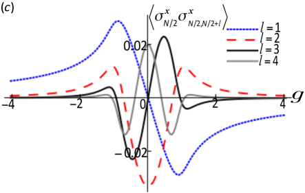
The appearance of the trivial state as an attractor at $g\to 0$, cannot be simply related to minimum or maximum energy states as in the earlier discussion. Note also that the above dualities do not explain why the same-sublattice correlators, which are even functions of $g$, should vanish at $g=0$. The state at $g=0$ can nonetheless be directly understood: at $g=0,\Delta=1$, the effective magnetic field seen by any site points purely in the $x$ direction, and so the evolution combines precession around the $x$ axis with decay. Consequently, the $x$ component of all spins vanishes at this point. The correlators $\langle\sigma^{y}_{j}\sigma^{y}_{j+l}\rangle$ (not shown) do not generally vanish at $g=0$, but still show the odd–even symmetry discussed above. For $\Delta<1$ the $\langle\sigma^{x}_{j}\sigma^{x}_{j+l}\rangle$ do not vanish at $g=0$ either; this is discussed further in Sec. III.4.

III.2 Comparison with the mean-field theory

To further understand the differences between the NESS and the ground state, we next discuss the mean-field prediction for the NESS. While mean-field theory incorrectly predicts long-range order in low dimensions, the nature of the order predicted is reflected by the full MPO numerics. Within mean-field theory it is possible to give closed-form expressions for the phase boundary, and for the nature of the order anticipated for given values of $g,\Delta,\kappa$. This provides further intuition for the differences between the NESS and the ground state.

In mean-field theory, the full density matrix is approximated as a product state (i.e. equivalent to restricting $\chi_{\text{max}}=1$ in an MPO simulation). The equations of motion then reduce to the following set of non-linear Bloch equations:

$$\frac{d}{dt}\langle\hat{\sigma}_{j}^{x}\rangle =\!-\tilde{\kappa}\langle\hat{\sigma}_{j}^{x}\rangle\!+\!2g\langle\hat{\sigma}_{j}^{y}\rangle\!-\!(1-\Delta)\langle\hat{\sigma}_{j}^{z}\rangle(\langle\hat{\sigma}_{j-1}^{y}\rangle+\langle\hat{\sigma}_{j+1}^{y}\rangle)$$

$$\frac{d}{dt}\langle\hat{\sigma}_{j}^{y}\rangle =\!-\tilde{\kappa}\langle\hat{\sigma}_{j}^{y}\rangle\!-\!2g\langle\hat{\sigma}_{j}^{x}\rangle\!+\!(1+\Delta)\langle\hat{\sigma}_{j}^{z}\rangle(\langle\hat{\sigma}_{j-1}^{x}\rangle+\langle\hat{\sigma}_{j+1}^{x}\rangle)$$

$$\frac{d}{dt}\langle\hat{\sigma}_{j}^{z}\rangle =\!-2\tilde{\kappa}(\langle\hat{\sigma}_{j}^{z}\rangle+1)-(1+\Delta)\langle\hat{\sigma}_{j}^{y}\rangle(\langle\hat{\sigma}_{j-1}^{x}\rangle+\langle\hat{\sigma}_{j+1}^{x}\rangle)$$

$$\!+(1-\Delta)\langle\hat{\sigma}_{j}^{x}\rangle(\langle\hat{\sigma}_{j-1}^{y}\rangle+\langle\hat{\sigma}_{j+1}^{y}\rangle).$$ (9)

One may either directly time-evolve these equations to determine steady states, or attempt to analytically solve these equations in cases where the spatial dependence is relatively simple. Below we first present the analytical approach, and then discuss direct numerical evolution.

It is clear from Eq. (III.2) that the trivial state $\langle\hat{\sigma}_{j}^{x}\rangle=\langle\hat{\sigma}_{j}^{y}\rangle=0,\langle\hat{\sigma}_{j}^{z}\rangle=-1$ is always a fixed point, i.e. a steady state. This trivial state does not break the $\mathbbm{Z}_{2}$ symmetry of Eq. (4) and so can also be referred to as a paramagnetic stateLee et al. (2013). While such a steady state always exists, this state need not always be stable to small fluctuations. To test linear stability, one may linearize the equations of motion around the steady state, and consider plane-wave fluctuations of the form:

$$\left(\begin{array}[]{c}\langle\hat{\sigma}_{j}^{x}\rangle\\ \langle\hat{\sigma}_{j}^{y}\rangle\\ \langle\hat{\sigma}_{j}^{z}\rangle\end{array}\right)=-\left(\begin{array}[]{c}0\\ 0\\ 1\end{array}\right)+\sum_{k}\left(\begin{array}[]{c}x_{k}\\ y_{k}\\ z_{k}\end{array}\right)e^{-i\nu_{k}t-ijk}.$$

The equations of motion then yield a secular equation for the frequencies $\nu_{k}$, with solutions

$$\nu_{k}=-i\tilde{\kappa}\pm 2\sqrt{g^{2}+2g\cos(k)+(1-\Delta^{2})\cos^{2}(k)}.$$ (10)

and $\nu_{k}=-2i\tilde{\kappa}$. The steady state is stable to such a plane wave fluctuation $k$ if $\Im[\nu_{k}]<0$, meaning such fluctuations exponentially decay.

It is clear that for $|\Delta|<1$, the trivial state is stable at both $g\to 0$ and $g\to\infty$. The trivial state can be unstable at intermediate $g$. For positive $g$, the most unstable fluctuations have $\cos(k)=-1$, i.e AFM fluctuations, whereas for negative $g$ FM fluctuations, $\cos(k)=1$ are the most unstable. In the Ising limit $\Delta=1$, one can write a simple expression for the phase boundary, $\tilde{\kappa}=2\sqrt{1-(g\pm 1)^{2}}$, indicating that for small enough $\tilde{\kappa}$ the normal state is unstable near to $g=\pm 1$.

In addition to the trivial state one may consider the FM ansatz $\langle\hat{\sigma}_{j}^{x}\rangle=X,\langle\hat{\sigma}_{j}^{y}\rangle=Y,\langle\hat{\sigma}_{j}^{z}\rangle=Z$, or AFM ansatz $\langle\hat{\sigma}_{j}^{x}\rangle=(-1)^{j}X,\langle\hat{\sigma}_{j}^{y}\rangle=(-1)^{j}Y,\langle\hat{\sigma}_{j}^{z}\rangle=Z$, and then find $X,Y,Z$ by substituting these forms into Eq. (III.2) and solving the resulting cubic equation. One finds that for negative $g$, there is a non-trivial FM solution ($X,Y\neq 0$), which exists only when the trivial state is unstable. (When the trivial state is stable, the cubic equation only has one real root corresponding to $X=Y=0,Z=-1$.) For $g>0$ the same statements apply to the AFM ansatz. Whenever these non-trivial solutions exist they can be shown to be stable.

This analysis predicts a simple phase diagram, corroborated by direct numerical time evolution of Eq. (III.2). There are three phases, trivial, FM and AFM. The boundaries between theses are given by the surfaces $\nu_{\pi}=0,\nu_{0}=0$ with $\nu_{k}$ from Eq. (10). This phase diagram is shown in Fig. 4 as a function of parameters $g,\Delta,\tilde{\kappa}$. It is clear that for a fixed $\tilde{\kappa}$ and with decreasing value of $\Delta$, the range of the transverse field strength $g$ over which the FM and AFM exist decreases. As $\Delta\to 0$, for finite $\kappa$, the trivial state always occurs regardless of the value $g$.

Figure 4: (Color online) Mean-field phase diagram for the non-equilibrium steady state of Eq. (4) as a function of dimensionless parameters $g,\Delta,\tilde{\kappa}$.

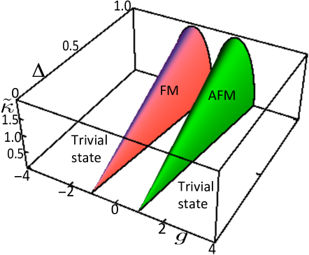
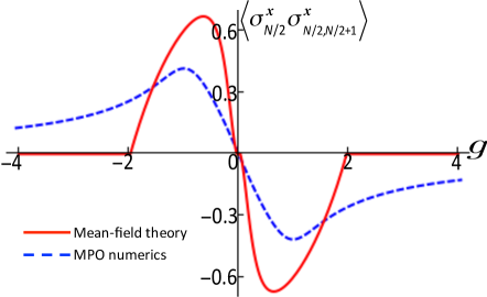
To compare the predictions of mean-field theory and the full numerics, Fig. 5 compares their predictions for the correlation function $\langle\hat{\sigma}_{j}^{x}\hat{\sigma}_{j+1}^{x}\rangle$ as a function of transverse field strength $g$. In the trivial state, MFT predicts this correlation to vanish, while in the ordered states it predicts $\pm X^{2}$, for the FM (AFM) states respectively. As can be seen, MFT does predict the kind of order that is seen, but predicts sharp phase boundaries that are not seen in the full numerics.

Figure 5: (Color online) Spin-spin correlations $\langle\sigma^{x}_{j}\sigma^{x}_{j+1}\rangle$ as a function of transverse field strength $g$. Parameters (in units of $J$): $\Delta=1,\tilde{\kappa}=0.5$ and MPO calculation performed for $N=40$ site chain, with $\chi_{\text{max}}=20$.

As noted above, direct time evolution of Eqs. (III.2) corroborate the above phase diagram. However, the steady state found does depend on the initial conditions used. Specifically, considering small periodic perturbations around the trivial state and time evolving Eq. (III.2) yields the AFM, trivial and FM states exactly as discussed above. In contrast, if time evolved from a random initial configuration, domains of FM/AFM can exist, separated by defect sites (domain walls). The dynamics of such domain walls becomes frozen within the mean-field numerics. The absence of long-range order seen in the full MPO numerics can be considered as the effect of a superposition of many different configurations of domain walls.

III.3 Correlations vs transverse field in the Ising limit

We now turn to the properties of quantum correlations at $\Delta=1$ (the Ising model). For comparison, we summarize here the ground state properties, as studied in Osterloh et al. (2002); Osborne and Nielsen (2002); Vidal et al. (2003). In the Ising model entanglement is short ranged: Only nearest and next-nearest neighboring spins are entangled. The magnitude of the nearest neighbor entanglement however shows critical scaling. At the critical point $|g|=1$ Ref. Osterloh et al. (2002) showed that $d\mathcal{C}/dg$ (where $\mathcal{C}$ is concurrence, another measure of entanglement) scaled as a power of the system size. Consequently, the peak value of $\mathcal{C}(g)$ actually occurs for $|g|>1$, rather than at the critical point. In the ground state, nearest neighbor entanglement only vanished at $g\to 0,|g|\to\infty$ Osterloh et al. (2002). Quantum discord for the same model was studied in Ref. Maziero et al. (2010). Discord is not restricted to nearest neighbors, and is peaked near $|g|=1$.

Figure 6: (Color online) Evolution of quantum correlations with transverse field $g$ in the Ising limit. Panel (a) shows negativity $\mathcal{N}$, panel (b) geometric quantum discord $\mathcal{D}$. In addition the integrated susceptibility $S^{xx}_{\text{int}}=\sum_{j}\langle\sigma_{i}^{x}\sigma_{j}^{x}\rangle$ is shown in (c); at the equilibrium critical point this would show a power law divergence with system size. Note that only one line is shown in panel (a) because entanglement vanishes beyond nearest neighbors at $\Delta=1$. Parameters as in Fig. 3.

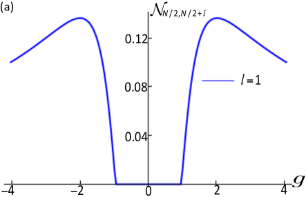
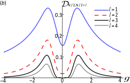
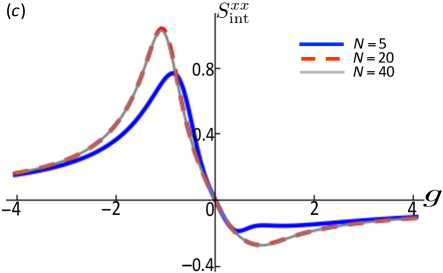
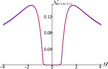
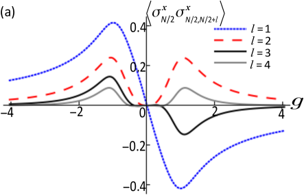
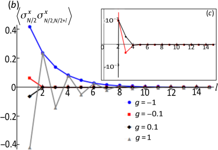
Figure 6 shows the evolution of quantum correlations (negativity  and geometric quantum discord) with transverse field $g$ in the non-equilibrium steady state at $\Delta=1,\tilde{\kappa}=0.5$. In addition, the integrated susceptibility $S^{xx}_{\text{int}}=\sum_{j}\langle\sigma_{i}^{x}\sigma_{j}^{x}\rangle$ (static spin structure factor) is shown. This correlation function both serves as an example of a correlation function that does not require specifically quantum correlations, and also as a function which would diverge (as a power law of system size) at the ground state critical point — such a divergence reflects the appearance of quasi-long range order in the spin-spin correlator. The asymmetry of this correlation function seen in Fig. 6(c) reflects the switch from ferromagnetic to antiferromagnetic order.

Despite the switch between ferro- and antiferromagnetic order with sign of $g$, which is absent in the ground state, several features of the quantum correlations match closely the ground state behavior. Entanglement has a short range, existing now only between nearest neighbors as shown in Fig. 6(a), while discord extends to greater separations Fig. 6(b). Negativity also peaks at a value $|g|>1$. These features exist for both signs of $g$; this is because the entanglement measures are not affected by the sublattice sign-changes induced by the duality discussed above. As discussed in Ref. Ma et al. (2011), two-mode squeezing is a sufficient condition for pairwise entanglement. We have confirmed that in the range of $g$ for which which bipartite entanglement vanishes, the two-mode spin squeezing parameter is identically zero.

In contrast to the ground state, there is however no critical behavior: the entanglement is an analytic function of $g$ with no singular behavior at $|g|=1$. Similarly, the integrated susceptibility does not diverge with increasing system size but instead saturates. This reflects exponential spatial decay of correlations, i.e. a finite correlation length, as anticipated due to the dissipation. The absence of critical behavior and the presence of only short range correlations suggests the NESS of this 1D system does not undergo any phase transition. Such a result is to be expected, since any finite temperature leads to short range order for a 1D system with short ranged interactions. Although we consider dissipation due to an empty (i.e. zero temperature) bath, we consider a non-equilibrium situation. As has been discussed elsewhere, see e.g. Dalla Torre et al. (2012, 2013), this leads to a non-zero low-energy effective temperature.

Also in contrast to the ground state behavior, for small $|g|$ entanglement vanishes entirely. The nature of this disappearance, i.e. the sharp threshold seen in Fig. 6(a) is a general feature of entanglement in a dissipative system Yu and Eberly (2009) — finite amounts of dissipation can make a state become separable. Discord however remains non-zero between nearest neighbors at $g=0$.

III.4 Correlations vs anisotropy (pump-strength) $\Delta$

In the ground state, the range of entanglement was found to grow as one moves away from the Ising limit ($\Delta=1$), toward the isotropic XY limit ($\Delta=0$) Osborne and Nielsen (2002). We therefore next explore how pump strength $\Delta$ affects the scale and range of correlations. Since the anisotropy parameter $\Delta$ is also the strength of pumping the isotropic limit corresponds to vanishing pump, the consequence of this double rôle of $\Delta$.

Figure 7: (Color online) Evolution of quantum correlations with transverse field $g$ near the isotropic limit, $\Delta=0.05$. Panels (a),(b) show negativity $\mathcal{N}$ and geometric quantum discord $\mathcal{D}$ as in Fig. 6. Panel (c) shows spin-spin correlation $\langle\sigma^{x}_{j}\sigma^{x}_{j+l}\rangle$ as in Fig. 3. Panel (d) shows spatial dependence of correlations for the anisotropic X-Y model. Parameters (in units of $J$): $\tilde{\kappa}=0.5$ and MPO calculation performed for $N=40$ site chain, with $\chi_{\text{max}}=20$.

We first consider how Fig. 6 is modified when $\Delta<1$. Figure 7 shows the behavior of entanglement, discord and correlation functions for $\Delta=0.05$, close to the isotropic limit. As discussed above, the $\langle\sigma^{x}_{N/2}\sigma^{x}_{N/2+l}\rangle$ still show the odd even symmetry, but the vanishing of all correlations at $g=0$ no longer occurs — the precession axis now lies within the $xy$ plane, and so the $x$ component of spin need not decay to zero. When $\Delta<1$, as in the ground state, entanglement extends over a larger range, i.e. not only between nearest neighbors. In addition, the peak entanglement now occurs near $g=0$, rather than at $|g|>1$, i.e. quantum correlations attain their maximal value away from the equilibrium quantum critical point Latorre et al. (2004). In addition, the peak value of entanglement (and all correlations) is significantly smaller than that seen at $\Delta=1$. From Fig. 7(c) it is clear that at large negative $g$ there is again short-range ferromagnetic order, and antiferromagnetic order at large positive $g$. At smaller $g$, just as seen at $\Delta=1$, the short-range ordering is incommensurate [see Fig. 7(d)]. However, the value of $|g|$ required to see FM/AFM order is larger for $\Delta=0.05$ than it was for $\Delta=1$, so that $g=\pm 1$ now shows incommensurate order.The correlations do still respect the sublattice duality discussed earlier. In contrast to the behavior at $\Delta=1$, the correlations always have a small magnitude [compare the scale of Fig. 7(c,d) as compared to Fig. 3]. This is consistent with the observation that for $\Delta=0.05,\tilde{\kappa}=0.5$, the mean-field theory would predict the trivial state independent of the value of $g$ (see Fig. 4).

Figure 8: (Color online) Evolution of quantum correlations with anisotropy $\Delta$. Panel (a) shows negativity $\mathcal{N}$ and (b) geometric quantum discord $\mathcal{D}$. Parameters (in units of $J$): $g=-1,\tilde{\kappa}=0.5$ and MPO calculation performed for $N=40$ site chain, with $\chi_{\text{max}}=20$.

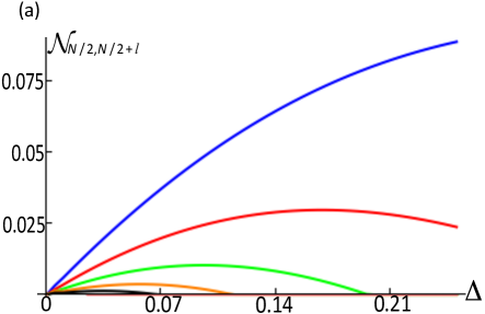
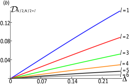
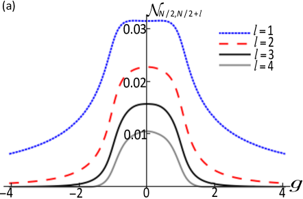
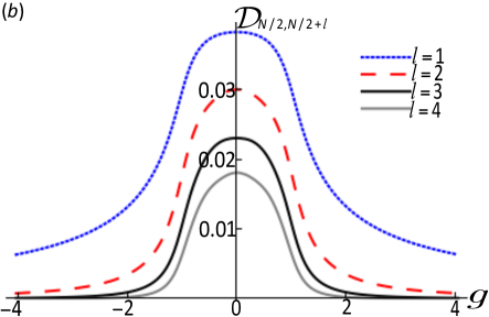
While $\Delta=0.05$ leads to a longer range of entanglement, the symmetry of the problem remains Ising-like for all $0<\Delta\leq 1$. In the ground state, the combination of this fact and universality together imply that the range of entanglement must remain finite as long as $\Delta$ is non-zero Maziero et al. (2010). The same behavior is indeed seen in the non-equilibrium steady state: For any non-zero $\Delta$, entanglement only extends over a finite range, this range grows as $\Delta$ shrinks and diverges at $\Delta\to 0$. This can be seen in Fig. 8 which shows the evolution of entanglement and discord as a function of $\Delta$ for various different separations between sites.

As anticipated above, the limit $\Delta\to 0$ is special, since $\Delta$ corresponds to pumping strength. Specifically, as $\Delta\to 0$, the range over which entanglement exists continues to grow, but the magnitude of the entanglement for any pair of sites ultimately vanishes. Thus the limit $\Delta\to 0$ is singular, with diverging range of correlations, but vanishing magnitude. The vanishing of negativity, and in fact of all correlations, at $\Delta=0$ can be easily understood from the equation of motion: at $\Delta=0$, the Hamiltonian conserves numbers of excited two-level systems, while the dissipation reduces this number, so the steady state must be the trivial empty state, which is a product state and thus uncorrelated.

The origin of growing range of negativity can be found by examining the structure and scaling of the two-site density matrix. We first note that this density matrix has a simple structure:

$$\rho_{ij}=\left(\begin{array}[]{cccc}p_{11}&0&0&x_{4}\\ 0&p_{10}&x_{5}&0\\ 0&x_{5}^{\ast}&p_{01}&0\\ x_{4}^{\ast}&0&0&p_{00}.\end{array}\right).$$ (11)

This structure is due to a symmetry of the equation of motion, under the transformation $\rho\to\hat{R}\rho\hat{R}$ with $\hat{R}=\prod_{j}\sigma^{z}_{j}$. The consequences of such a symmetry for the Hamiltonian were previously discussed Osborne and Nielsen (2002); the decay terms we consider also respect this symmetry. Consequently the steady state density matrix should satisfy $[R,\rho]=0$. Tracing over all but two sites, $[\sigma^{z}_{i}\sigma^{z}_{j},\rho_{ij}]=0$, which imposes the structure discussed above. A state of the form (11) is entangled iff either $p_{10}p_{01}<|x_{4}|^{2}$ or $p_{00}p_{11}<|x_{5}|^{2}$. In the limit of small $\Delta$ the excited state populations $p_{11},p_{01},p_{10}\sim\Delta^{2}$ and so $p_{00}\sim 1$. The off diagonal matrix elements scale as $|x_{4}|\sim\Delta,|x_{5}|\sim\Delta^{2}$. All of these expressions have prefactors that depend on the separation between sites. However, regardless of these prefactors, the scaling of $p_{01},p_{10},x_{4}$ with $\Delta$ implies that as $\Delta\to 0$, the first of the two criteria above will always be satisfied, i.e. for any pair of sites, there exists a $\Delta_{c}$ such that for $0<\Delta<\Delta_{c}$ they will be entangled. Furthermore, as discussed in section IV, this behavior can be derived analytically within a spin-wave approximation.

III.5 Correlations vs decay rate

Figure 9: (Color online) Evolution of quantum correlations with $\tilde{\kappa}$. Panel (a) shows negativity $\mathcal{N}$, and panel (b) shows geometric quantum discord $\mathcal{D}$, for both Ising limit and small anisotropy limit. Parameters (in units of $J$): $g=-1$ and MPO calculation performed for $N=40$ site chain, with $\chi_{\text{max}}=20$.

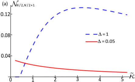
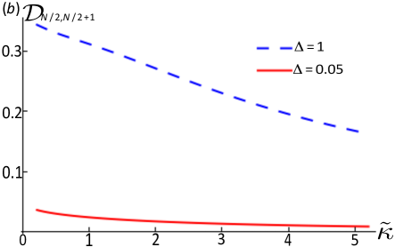
Having explored the dependence on the parameters $\Delta,g$, we conclude our discussion of numerical results by presenting the dependence of quantum correlations on the decay rate $\tilde{\kappa}=\kappa/J$. Figure 9 shows the evolution with decay rate at $g=-1$, and the two values of $\Delta$ shown in detail above. Whereas the discord decreases monotonically with decay rate, the behavior of the negativity depends on anisotropy. In particular, in the Ising limit, there is a non-monotonic dependence, exhibiting a separable but non-classical state for sufficiently small $\tilde{\kappa}$. The appearance of non-zero entanglement with increasing $\tilde{\kappa}$ corresponds to the condition $p_{01}p_{10}=|x_{4}|^{2}$: on increasing $\tilde{\kappa}$, the probabilities $p_{01}\equiv p_{10}$ decrease while $|x_{4}|$ varies little at small $\tilde{\kappa}$. Non-monotonic dependence of entanglement on decay rate has also been seen in other contexts Joshi et al. (2013). Note that the decay terms remain important even at $\tilde{\kappa}\to 0$. In this limit the steady state is only attained at long times; the state which is finally attained is still determined by the open system dynamics.

IV Asymptotic $\Delta\to 0$ behavior and spin-wave approximation

IV.1 Spin-wave calculation of negativity

As noted above, for $\Delta=0$, the NESS of our model corresponds to an empty state. This suggests that for small $\Delta$ an approximation based on a low density of excited two-level systems can be used: a bosonic spin-wave approach Mattis (2006). This corresponds to reverting from two-level systems (hard core bosons) to bosonic fields $\sigma_{j}^{-}\rightarrow\hat{b}_{j}$. Equation (2) thus becomes:

$$H_{\text{eff}}=-\sum_{j}\left[g(2\hat{b}_{j}^{\dagger}\hat{b}_{j}-1)+\left(\hat{b}_{j}^{\dagger}\hat{b}_{j+1}+\hat{b}_{j+1}^{\dagger}\hat{b}_{j}\right)\right.\\ \left.{}+\Delta(\hat{b}_{j}^{\dagger}\hat{b}_{j+1}^{\dagger}+\hat{b}_{j+1}\hat{b}_{j})\right].$$ (12)

This approximation is valid as long as double occupancy of a site can be ignored. Fourier transforming both this and the loss term, the Master equation can be written as:

$$\frac{d\rho}{dt} =-i[\sum_{k}h_{k},\rho]+\tilde{\kappa}\!\sum_{k}[2\hat{b}_{k}{\rho}\hat{b}_{k}^{\dagger}-\hat{b}_{k}^{\dagger}\hat{b}_{k}\rho-\rho\hat{b}_{k}^{\dagger}\hat{b}_{k}]$$ (13)

$$h_{k} =-\left(\begin{array}[]{cc}\hat{b}^{\dagger}_{k}&\hat{b}_{-k}\end{array}\right)\left(\begin{array}[]{cc}g+\cos(k)&\Delta\cos(k)\\ \Delta\cos(k)&g+\cos(k)\end{array}\right)\left(\begin{array}[]{c}\hat{b}_{k}\\ \hat{b}^{\dagger}_{-k}\end{array}\right),$$ (19)

so that each pair of modes $k,-k$ form a closed subsystem.

To find steady state correlations, we replace the density matrix equation of motion, Eq. (13), by equivalent Heisenberg-Langevin equations Scully and Zubairy (1997). The Heisenberg-Langevin equations can be derived by writing the Heisenberg equations for the system operators coupled to a Markovian bath. After eliminating the dynamics of the bath operators, one finds equations for the system operators of the form:

$$\frac{d}{dt}\hat{b}_{k}=i[h_{k}+h_{-k},\hat{b}_{k}]-\tilde{\kappa}\hat{b}_{k}+\sqrt{2\tilde{\kappa}}\hat{b}_{k}^{in}(t).$$ (20)

The Markovian bath has two effects: it causes decay of the system operator $\hat{b}_{k}$ at the rate $\tilde{\kappa}$, and it introduces an “input noise” term $\hat{b}_{k}^{in}(t)$. Since we consider decay into an zero temperature (i.e. empty) bath, there is only vacuum quantum noise: the only non-zero noise correlation function is $\langle\hat{b}_{k}^{in}(t)\hat{b}_{k^{\prime}}^{\dagger in}(t^{\prime})\rangle=\delta_{k,k^{\prime}}\delta(t-t^{\prime})$. Because of the anomalous (pumping) terms in Eq. (12), the equation for $\hat{b}_{k}$ couples to that for $\hat{b}_{-k}^{\dagger}$ and vice versa. The coupled equations for operators $\hat{b}_{k}$ and $\hat{b}_{-k}^{\dagger}$ can be written in a matrix form,

$$\dot{\hat{f}}(t) =\mathcal{M}\hat{f}(t)+\hat{m}(t),$$ (21)

in which $\hat{f}(t)$ is the column vector comprising operators $\hat{b}_{k}(t)$ and $\hat{b}_{-k}^{\dagger}(t)$, $\hat{m}(t)$ is the column vector containing the noise operators:

$$\hat{f}(t) =\!\left(\!\begin{array}[]{cc}\hat{b}_{k}(t),&\hat{b}_{-k}^{\dagger}(t)\end{array}\!\!\right)^{T}$$ (23)

$$\hat{m}(t) =\!\left(\!\begin{array}[]{cc}\sqrt{2\tilde{\kappa}}\hat{b}_{k}^{in}(t),&\sqrt{2\tilde{\kappa}}\hat{b}_{-k}^{\dagger in}(t)\end{array}\!\!\right)^{T};$$ (25)

and the matrix $\mathcal{M}$ is given by

$$\mathcal{M}=\left(\!\begin{array}[]{cc}-\tilde{\kappa}+2i(g+\cos(k))&2i\Delta\cos(k)\\ -2i\Delta\cos(k)&-\tilde{\kappa}-2i(g+\cos(k))\end{array}\!\!\right).$$ (28)

The solution of Eq. (21) is $\hat{f}(t)=e^{\mathcal{M}t}\hat{f}(0)+\int_{0}^{t}e^{\mathcal{M}(t-t^{\prime})}\hat{m}(t^{\prime})dt^{\prime}$. Since the real parts of the eigenvalues of $\mathcal{M}$ are negative, the first of these terms vanishes in the long time limit $t\to\infty$. In this limit one then finds:

$$\frac{\hat{b}_{k}(t)}{\sqrt{2\tilde{\kappa}}} =\!\int_{0}^{t}\!\!dt^{\prime}\left[\mathcal{G}_{1}(t-t^{\prime})\hat{b}_{k}^{in}(t^{\prime})+\mathcal{G}_{2}(t-t^{\prime})\hat{b}_{-k}^{\dagger in}(t^{\prime})\right]$$

$$\frac{\hat{b}_{-k}^{\dagger}(t)}{\sqrt{2\tilde{\kappa}}} =\!\int_{0}^{t}\!\!dt^{\prime}\left[\mathcal{G}_{1}^{\ast}(t-t^{\prime})\hat{b}_{-k}^{\dagger in}(t^{\prime})+\mathcal{G}_{2}^{\ast}(t-t^{\prime})\hat{b}_{k}^{n}(t^{\prime}))\right]$$ (29)

where the propagators $\mathcal{G}_{1,2}(\tau)$ are matrix elements of $\exp(M\tau)$. By introducing the dispersions $\epsilon_{k}=2(g+\cos(k)),\eta_{k}=2\Delta\cos(k),\xi_{k}=\sqrt{\epsilon_{k}^{2}-\eta_{k}^{2}},$ the propagators can be written as:

$$\mathcal{G}_{1}(\tau) =e^{-\tilde{\kappa}\tau}\left[\cos(\tau\xi_{k})+i\epsilon_{k}\frac{\sin\left(\tau\xi_{k}\right)}{\xi_{k}}\right]$$

$$\mathcal{G}_{2}(\tau) =i\eta_{k}e^{-\tilde{\kappa}\tau}\sin(\tau\xi_{k})/\xi_{k}.$$

To find the quantum correlations of the state, we first note that since the problem involves non-interacting bosons, the steady state is Gaussian, i.e. it can be fully characterized by the covariance matrix $V_{j,k}$ as given below. Introducing $\hat{x}_{j}=\hat{b}_{j}+\hat{b}^{\dagger}_{j},\hat{p}_{j}=(\hat{b}_{j}-\hat{b}^{\dagger}_{j})/i$ we have

$$V_{j,k}=\!\left(\!\begin{array}[]{cc}{\bf A}_{j}&{\bf C}_{jk}\\ {\bf C}_{jk}^{T}&{\bf A}_{k}\end{array}\!\!\right)\!,\quad{\bf C}_{jk}=\!\left(\!\begin{array}[]{cc}\langle x_{j}x_{k}\rangle_{s}&\langle x_{j}p_{k}\rangle_{s}\\ \langle x_{k}p_{j}\rangle_{s}&\langle p_{j}p_{k}\rangle_{s}\end{array}\!\!\right),$$ (30)

and ${\bf A}_{j}={\bf C}_{jj}$ where $\langle xp\rangle_{s}=\langle xp+px\rangle/2$. To find these correlators, it is sufficient to find $\langle\hat{b}_{j}^{\dagger}\hat{b}_{j+l}\rangle$, and $\langle\hat{b}_{j}\hat{b}_{j+l}\rangle$. In the real space the correlator $\langle\hat{b}_{j}^{\dagger}\hat{b}_{j+l}\rangle$ can be expressed as

$$\langle\hat{b}_{j}^{\dagger}\hat{b}_{j+l}\rangle=\frac{1}{N}\sum_{k,k^{\prime}}\langle\hat{b}_{k}^{\dagger}\hat{b}_{k^{\prime}}\rangle e^{i(k^{\prime}-k)j}e^{ik^{\prime}l}.$$ (31)

Using Eq. (29) one finds that for $N\to\infty$:

$$\langle\hat{b}_{j}^{\dagger}\hat{b}_{j+l}\rangle=\frac{1}{4\pi}\int_{-\pi}^{\pi}\frac{\eta_{k}^{2}}{\xi_{k}^{2}+\tilde{\kappa}^{2}}dke^{ikl}$$ (32)

and a similar expression for $\langle\hat{b}_{j}\hat{b}_{j+l}\rangle$. By substituting $e^{ik}\to z$, the integral becomes a contour integral around the unit circle $|z|=1$, so its value depends on the residue of those poles $z=Z$ with $|Z|<1$. The four poles come in complex conjugate pairs and can be found in closed form $Z=\zeta\pm\sqrt{\zeta^{2}-1}$ where $\zeta=\left[g\pm\sqrt{g^{2}\Delta^{2}-\tilde{\kappa}^{2}(1-\Delta^{2})/4}\right]/(1-\Delta^{2})$. Two of these poles which we denote as $Z_{0},Z_{0}^{\ast}$ lie within the unit circle, and in terms of these one finds:

$$\langle\hat{b}_{j}^{\dagger}\hat{b}_{j+l}\rangle =\Delta^{2}\left[\alpha(Z_{0})^{l-1}+\alpha^{*}(Z_{0}^{*})^{l-1}\right]$$ (33)

$$\langle\hat{b}_{j}\hat{b}_{j+l}\rangle =\Delta\beta(Z_{0}^{*})^{l-1}$$ (34)

where $\alpha,\beta$ are complex functions of $\tilde{\kappa},\Delta,g$. We have factored out the asymptotic scaling with $\Delta$ at $\Delta\to 0$. Since $|Z_{0}|<1$, all correlations decay exponentially with separation $n$.

The definition of negativity given earlier, Eq. (5), is specific to qubits, i.e. two-level systems. For a Gaussian state an alternate definition of negativity can be found in terms of the symplectic eigenvalue $\tilde{\nu}_{-}^{2}=(\tau-\sqrt{\tau^{2}-4{\rm Det}[V_{j,j+l}]})/2$, where $\tau={\rm Det}[A_{j}]+{\rm Det}[A_{j+l}]-2{\rm Det}[C_{j,j+l}]$. The state is separable if $\tilde{\nu}_{-}>1$, and so negativity for such states may be defined as $\mathcal{N}=\text{max}(0,1-\tilde{\nu}_{-})$. Using the asymptotic scaling of the elements of the covariance matrix with $\Delta$, we find that in the $\Delta\to 0$ limit

$$\tilde{\nu}_{-}\simeq\sqrt{1-4|\langle\hat{b}_{j}\hat{b}_{j+l}\rangle|^{2}},\quad\mathcal{N}\simeq 2|\langle\hat{b}_{j}\hat{b}_{j+l}\rangle|$$ (35)

Within this limit, it is thus clear that $\mathcal{N}>0$ for all pairs of sites, but $\mathcal{N}\propto\Delta$ and so $\mathcal{N}$ vanishes at small $\Delta$, reproducing the singular behavior found numerically in the previous section.

IV.2 Comparing spin-wave approximation to numerics

The spin wave theory relies on neglecting effects of possible double occupation of a given site. While the probability of such an event is small for $\Delta\to 0$, it is not a-priori clear whether its effects are negligible, since the pair creation term creates excitations on adjacent sites, hence hopping can easily create a doubly occupied site within the bosonic approximation. For this reason, we a compare the results of the MPO numerics and the spin-wave theory in the limit $\Delta\to 0$.

We focus on the correlation function $\langle\sigma_{j}^{-}\sigma_{j+l}^{-}\rangle$, or its equivalent bosonic form, which according to Eq. (35) determines the asymptotic negativity as $\Delta\to 0$. Both MPO and spin-wave results show this correlation function decays exponentially with separation $l$ (neglecting edge effects). Consequently this correlation function can be characterized by its value for nearest neighbors $l=1$ (NB the $l=0$ case vanishes by definition), and by its correlation length $\xi_{c}$, defined as $|\langle\sigma_{j}^{-}\sigma_{j+l}^{-}\rangle|\propto e^{-l/\xi_{c}}$. In the spin-wave theory $\xi_{c}=-1/\ln[Z_{0}]$. These two characteristic quantities are shown in Fig. 10, focussing on the limiting behavior at $\Delta\to 0$.

Figure 10: (Color online) Panel (a) correlation length $\xi_{c}$ at $\Delta=0.005$ vs decay rate $\tilde{\kappa}$. Panel (b) Nearest neighbor correlations $|\langle\sigma_{j}^{-}\sigma_{j+1}^{-}\rangle|$ vs anisotropy $\Delta$ for several values of $\tilde{\kappa}$. In both panels MPO numerics (points) are compared to spin-wave theory (lines). Parameters (in units of $J$): $g=-1$, MPO calculation is performed for $N=40$ site chain with $\chi_{\text{max}}=20$.

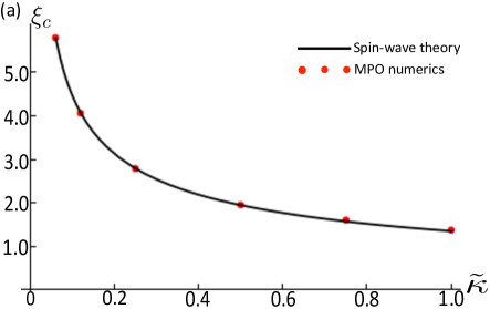
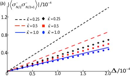
The correlation length shown in Fig. 10 shows that the spin-wave theory accurately reproduces the results of the numerics, and both show a diverging correlation length ($|Z_{0}|\to 1$) in the limit $\tilde{\kappa}\to 0$. In contrast, the magnitude of correlations (i.e. prefactors of the exponential decay) do not match well except at $\tilde{\kappa}\gg 1$. This can be explained as follows: at small $\tilde{\kappa}$, excitations created on adjacent sites can easily hop to create doubly occupied sites and thus rendering the bosonic approximation inaccurate. For $\tilde{\kappa}\gg 1$, excitations on adjacent sites are lost before hopping can create doubly excited sites.

V Conclusions

In the present work we have studied the non-equilibrium steady state of parametrically driven 1-D coupled cavity array. Making use of an MPO representation to determine the open system evolution, we obtain the non-equilibrium steady state of a dissipative transverse field Ising model. The steady state can be related to the ground state configuration for transverse field $g<0$, and to the maximum energy configuration for $g>0$. Consequently, for either sign of $g$, many features of the quantum correlations behave similarly to those in the ground state Ising model. The most significant difference is that dissipation destroys the phase transition, and so no critical behavior occurs at $|g|=1$ with correlation lengths remaining finite. We have also compared the results of the MPO numerics with the predictions of the mean-field theory. Mean-field theory erroneously predicts long-range ordered phases, but the nature of the ordering predicted is reflected by the MPO numerics. We have identified a singular limit, of weak driving, where the range of quantum correlations diverges, but the magnitude of the correlations vanishes. This limiting behavior can be recovered analytically from a spin wave theory, which accurately recovers the correlation length in this limit.