Disaggregated Bundle Methods for
Distributed Market Clearing in Power Networks

Abstract

A fast distributed approach is developed for the market clearing with large-scale demand response in electric power networks. In addition to conventional supply bids, demand offers from aggregators serving large numbers of residential smart appliances with different energy constraints are incorporated. Leveraging the Lagrangian relaxation based dual decomposition, the resulting optimization problem is decomposed into separate subproblems, and then solved in a distributed fashion by the market operator and each aggregator aided by the end-user smart meters. A disaggregated bundle method is adapted for solving the dual problem with a separable structure. Compared with the conventional dual update algorithms, the proposed approach exhibits faster convergence speed, which results in reduced communication overhead. Numerical results corroborate the effectiveness of the novel approach.

I Introduction

Demand response (DR) has been identified as an important resource management task in modern power networks promising to enable end-user interaction with the grid. DR aggregators serving large numbers of residential users will be able to participate in the market clearing by offering bids depending on the elasticity for power consumption of their end users. Bidirectional communication between aggregators and users is provided by the Advanced Metering Infrastructure (AMI) [1], with smart meters used as the end-users’ terminals.

The principal challenge for large-scale incorporation of DR from residential end-users is to account for the user scheduling preferences and intertemporal flexibility in a way that also protects user privacy. The advantages of intertemporal load scheduling flexibility are for instance demonstrated in [2, 3], but without considering small-scale users and pertinent distributed algorithms. Aggregation of small-scale user loads into the system scheduling has been the theme of [4, 5], but an array of issues ranging from incorporation of user utility functions and user privacy to algorithm convergence, are not fully addressed. Algorithms for market clearing with large-scale integration of DR from small loads with different utility functions are developed in [6] based on Lagrangian dual decomposition. The disaggregated cutting plane method (CPM) is proposed therein for updating the Lagrange multipliers.

This paper proposes a market clearing approach distributed among the market operator, aggregators, and the user smart meters by building upon the earlier work in [6]. Each end-user has preferences for smart appliance scheduling captured by utility functions and intertemporal constraints. The objective is to minimize the social net cost for day-ahead market clearing, while transmission network constraints are included in the form of DC power flows. To cope with the challenges of respecting end-user privacy and large-scale DR, dual decomposition is applied to the resulting optimization problem. Leveraging Lagrangian relaxation of the coupling constraints, the large-scale optimization decomposes into manageable small problems solved by the market operator (MO) and the aggregators in conjunction with the residential smart meters. Exploiting the separable structure of the problem at hand, a disaggregated bundle method is introduced for solving the dual problem with guaranteed convergence of the Lagrange multipliers. The developed solver yields faster convergence than its CPM counterpart, implying less communication overhead between the MO and the aggregators.

The remainder of this paper is organized as follows. Section II presents the market clearing problem involving large-scale DR. The decomposition algorithm along with the disaggregated bundle method solver is developed in Section III. Numerical tests are in Section IV, while conclusions and future directions are offered in Section V.

II Market Clearing Formulation

Consider a power network comprising $N_{g}$ generators, $N_{b}$ buses, $N_{l}$ lines, and $N_{a}$ aggregators, each serving a large number of residential end-users with controllable smart appliances. The scheduling horizon of interest is $\mathcal{T}:=\{1,2,\ldots,T\}$ (e.g., one day ahead). Let $\mathbf{p}_{G}^{t}:=[P_{G_{1}}^{t},\ldots,P_{G_{N_{g}}}^{t}]^{\prime}$ and $\mathbf{p}_{\mathrm{DRA}}^{t}:=[P_{\mathrm{DRA}_{1}}^{t},\ldots,P_{\mathrm{DRA}_{N_{a}}}^{t}]^{\prime}$ denote the generator power outputs, and the power consumption of the aggregators at slot $t$, respectively. Define further the sets $\mathcal{N}_{a}:=\{1,2,\ldots,N_{a}\}$ and $\mathcal{N}_{g}:=\{1,2,\ldots,N_{g}\}$. Each aggregator $j\in\mathcal{N}_{a}$ serves a set $\mathcal{R}_{j}$ of residential users, and each user $r\in\mathcal{R}_{j}$ has a set $\mathcal{S}_{rj}$ of controllable smart appliances. Let $\mathbf{p}_{jrs}$ be the power consumption of smart appliance $s$ and user $r$ corresponding to aggregator $j$ across the horizon. The power consumption $\mathbf{p}_{jrs}$ of each smart appliance across the horizon must typically satisfy operating constraints captured by a set $\mathcal{P}_{jrs}$, and may also give rise to user satisfaction represented by a concave utility function $B_{jrs}(\mathbf{p}_{jrs})$. Moreover, the generation cost is captured by convex functions $\{C_{i}(\cdot)\}_{i}$, and the fixed base load demands across the network buses at slot $t$ is denoted by the vector $\mathbf{p}_{\mathrm{BL}}^{t}$.

For brevity, vector $\mathbf{p}_{0}$ is used to collect all $p_{G_{i}}^{t}$, $P_{\mathrm{DRA}_{j}}^{t}$, and network nodal angles $\theta_{n}^{t}$; while vector $\mathbf{p}_{j}$ ($j\in\mathcal{N}_{a}$) collects all smart appliance consumptions corresponding to aggregator $j$. With the goal of minimizing the system net cost, the DC optimal power flow (OPF) based market clearing stands as follows:

$$f^{*}= \min_{\{\mathbf{p}_{j}\}_{j=0}^{N_{a}}}\sum_{t=1}^{T}\sum_{i=1}^{N_{g}}C_{i}(P_{G_{i}}^{t})-\sum_{j=1}^{N_{a}}\sum_{r\in\mathcal{R}_{j}}\sum_{s\in\mathcal{S}_{jr}}B_{jrs}(\mathbf{p}_{jrs})$$ (1a)

s. t. $$\mathbf{A}_{g}\mathbf{p}_{G}^{t}-\mathbf{A}_{a}\mathbf{p}_{\mathrm{DRA}}^{t}-\mathbf{p}_{\mathrm{BL}}^{t}=\mathbf{B}\bm{\theta}^{t},~{}t\in\mathcal{T}$$ (1b)

$$P_{G_{i}}^{\min}\leq P_{G_{i}}^{t}\leq P_{G_{i}}^{\max},~{}i\in\mathcal{N}_{g},~{}t\in\mathcal{T}$$ (1c)

$$-\mathsf{R}_{i}^{\mathrm{down}}\leq P_{G_{i}}^{t}-P_{G_{i}}^{t-1}\leq\mathsf{R}_{i}^{\mathrm{up}},~{}i\in\mathcal{N}_{g},\>t\in\mathcal{T}$$ (1d)

$$\mathbf{f}^{\min}\leq\mathbf{H}\bm{\theta}^{t}\leq\mathbf{f}^{\max},~{}t\in\mathcal{T}$$ (1e)

$$\theta_{1}^{t}=0,\>t\in\mathcal{T}$$ (1f)

$$0\leq P_{\mathrm{DRA}_{j}}^{t}\leq P_{\mathrm{DRA}_{j}}^{\max},~{}j\in\mathcal{N}_{a},\,t\in\mathcal{T}$$ (1g)

$$P_{\mathrm{DRA}_{j}}^{t}=\sum\nolimits_{r\in\mathcal{R}_{j},\,s\in\mathcal{S}_{jr}}{p}_{jrs}^{t},~{}j\in\mathcal{N}_{a},\>t\in\mathcal{T}$$ (1h)

$$\mathbf{p}_{jrs}\in\mathcal{P}_{jrs},\>r\in\mathcal{R}_{j},s\in\mathcal{S}_{jr},~{}j\in\mathcal{N}_{a}.$$ (1i)

Linear equality (1b) represents the nodal balance constraint. Limits of generator outputs and ramping rates are specified in constraints (1c) and (1d). Network line flow constraints are accounted for in (1e). Without loss of generality, the first bus can be set as the reference bus with zero phase (1f). Constraint (1g) captures the lower and upper bounds on the energy consumed by the aggregators. Equality (1h) amounts to the aggregator-users power balance equation; finally, (1i) gives the smart appliance constraints.

A smart appliance example is charging a PHEV battery, which typically amounts to consuming a prescribed total energy $E_{jrs}$ over a specific horizon from a start time $T_{jrs}^{\mathrm{st}}$ to a termination time $T_{jrs}^{\mathrm{end}}$. The consumption must remain within a range between $p_{jrs}^{\mathrm{min}}$ and $p_{jrs}^{\mathrm{max}}$ per period. With $\mathcal{T}_{E}:=\{T_{jrs}^{\mathrm{st}},\ldots,T_{jrs}^{\mathrm{end}}\}$, set $\mathcal{P}_{jrs}$ takes the form

$$\mathcal{P}_{jrs}=\Biggl{\{}\mathbf{p}_{jrs}\Biggl{|}\Biggr{.}\sum_{t\in\mathcal{T}_{E}}{p}_{jrs}^{t} =E_{jrs};\,p_{jrs}^{t}\in[p_{jrs}^{\mathrm{min}},p_{jrs}^{\mathrm{max}}],\,\forall~{}t\in\mathcal{T}_{E};$$

$$p_{jrs}^{t}=0,~{}\forall~{}t\in\mathcal{T}\setminus\mathcal{T}_{E}\Biggr{\}}.$$ (2)

Further examples of $\mathcal{P}_{jrs}$ and $B_{jrs}(\mathbf{p}_{jrs})$ can be found in [6], where it is argued that $\mathcal{P}_{jrs}$ is a convex set for several appliance types of interest.

Matrices $\mathbf{B}$ and $\mathbf{H}$ are defined as follows. With $X_{mn}$ denoting the reactance of line $(m,n)$, the bus admittance matrix $\mathbf{B}\in\mathbb{R}^{N_{b}\times N_{b}}$ has elements

$$[\mathbf{B}]_{mn}=-X_{mn}^{-1},\>\text{if $m\neq n$};~{}\quad[\mathbf{B}]_{mm}=\sum_{n=1}^{N_{b}}X_{mn}^{-1}$$

where $X_{mn}^{-1}:=0$ if line $(m,n)$ does not exist. Matrix $\mathbf{H}\in\mathbb{R}^{N_{l}\times N_{b}}$ has entries so that if line $q=1,\ldots,N_{l}$ connects buses $n$ and $n^{\prime}$, then

$$[\mathbf{H}]_{qm}=\begin{cases}X_{nn^{\prime}}^{-1},\text{~{}if $m=n$}\\ -X_{nn^{\prime}}^{-1},\text{~{}if $m=n^{\prime}$}\\ 0,\text{~{}otherwise}.\end{cases}$$

Finally, examples detailing the entries of matrices $\mathbf{A}_{g}$ and $\mathbf{A}_{a}$ in (1b) can be found in [6].

Problem (1) can be principally solved at the MO in a central fashion. However, there are two major challenges when it comes to solving (1) with large-scale DR: i) functions $B_{jrs}(\mathbf{p}_{jrs})$ and sets $\mathcal{P}_{jrs}$ are private, and cannot be revealed to the MO; ii) including the sheer number of variables $\mathbf{p}_{jrs}$ would render the overall problem intractable for the MO, regardless of the privacy issue. The aggregator plays a critical role in successfully addressing these two challenges through decomposing the optimization tasks that arises, as detailed in the ensuing section.

III Decomposition Algorithm

III-A Dual Decomposition

Leveraging the dual decomposition technique, problem (1) can be decoupled into simpler subproblems tackled by the MO and the aggregators. Specifically, consider dualizing the linear coupling constraint (1h) with corresponding Lagrange multiplier $\mu_{j}^{t}$. Upon straightforward re-arrangements, the partial Lagrangian can be written as

$$L(\{\mathbf{p}_{j}\}_{j=0}^{N_{a}},\bm{\mu})=L_{0}(\mathbf{p}_{0},\bm{\mu})+\sum_{j=1}^{N_{a}}L_{j}(\mathbf{p}_{j},\bm{\mu})$$ (3)

where

$$L_{0}(\mathbf{p}_{0},\bm{\mu}) :=\sum_{t=1}^{T}\left[\sum_{i=1}^{N_{g}}C_{i}(P_{G_{i}}^{t})-\sum_{j=1}^{N_{a}}\mu_{j}^{t}P_{\mathrm{DRA}_{j}}^{t}\right]$$ (4)

$$L_{j}(\mathbf{p}_{j},\bm{\mu}) :=\sum_{r\in\mathcal{R}_{j}}\sum_{s\in\mathcal{S}_{jr}}\left[\sum_{t=1}^{T}\mu_{j}^{t}{p}_{jrs}^{t}-B_{jrs}(\mathbf{p}_{jrs})\right].$$ (5)

The dual function is thus obtained by minimizing the partial Lagrangian over the primal variables $\{\mathbf{p}_{j}\}_{j=0}^{N_{a}}$ as

$$D(\bm{\mu}): =D_{0}(\bm{\mu})+\sum_{j=1}^{N_{a}}D_{j}(\bm{\mu})$$ (6a)

$$=\min_{\text{s.t. \eqref{eq:mc-bus}--\eqref{eq:mc-DRAlim}}}L_{0}(\mathbf{p}_{0},\bm{\mu})+\sum_{j=1}^{N_{a}}\min_{\text{s.t. \eqref{eq:mc-appl}}}L_{j}(\mathbf{p}_{j},\bm{\mu}).$$ (6b)

The dual decomposition essentially iterates between two steps: S1) Lagrangian minimization with respect to $\{p_{j}\}_{j=0}^{N_{a}}$ given the current multipliers, and S2) multiplier update, using the obtained primal minimizers. It is clear from (3) that the Lagrangian minimization can be decoupled into $1+N_{a}$ minimizations, where one is performed by the MO, and the rest by the corresponding aggregators.

Specifically, let $k=1,2,\ldots$ index iterations. Given the multipliers $\bm{\mu}(k)$, the subproblems at iteration $k$ solved by the MO and each residential end-user are given as follows

$$\mathbf{p}_{0}(k) =\operatorname*{arg\,min}_{\mathbf{p}_{0},~{}\text{s.t.~{}\eqref{eq:mc-bus}--\eqref{eq:mc-DRAlim}}}L_{0}(\mathbf{p}_{0},\bm{\mu}(k)) \{\mathbf{p}_{jrs}(k)\}_{s} =\operatorname*{arg\,min}_{\{\mathbf{p}_{jrs}\in\mathcal{P}_{jrs}\}_{s}}\sum_{s\in\mathcal{S}_{jr}}\Big{[}\sum_{t=1}^{T}\mu_{j}^{t}(k){p}_{jrs}^{t}-B_{jrs}(\mathbf{p}_{jrs})\Big{]}.$$ (7a) (7b)

Note that subproblem (7a) is a standard DC-OPF while the convex subproblem (7b) can be handled efficiently by the smart meters. In fact, with the feasible set in (2) and upon setting $B_{jrs}(\mathbf{p}_{jrs})\equiv 0$, (7b) boils down to the fractional knapsack problem, which can be solved in closed form. To this end, the multipliers $\mu_{j}^{t}(k)$ needed can be transmitted to the user’s smart meter via the AMI.

With the obtained quantities of $\mathbf{p}_{0}(k)$, $\{\mathbf{p}_{jrs}(k)\}_{s}$, and $\{D_{j}(\bm{\mu}(k))\}_{j=0}^{N_{a}}$, the ensuing section develops the approach to updating the multipliers $\{\mu_{j}^{t}\}_{j,t}$ using the so-termed bundle methods.

III-B Multiplier Update via Bundle Methods

The choice of the multiplier update method is crucial, because fewer update steps imply less communication between the CPM and the aggregators. A popular method of choice in the context of dual decomposition is the subgradient method, which is very slow typically. In this paper, the bundle method with disaggregated cuts is proposed for the multiplier update. It is better suited to the problem of interest yielding faster convergence, because it exploits the special structure of the dual function which can be written as a sum of separate terms [cf. (6)], while it overcomes the drawbacks of the cutting plane one developed in [6]. Numerical tests in Section IV illustrate differences in terms of convergence speed.

The following overview of the disaggregated bundle method in a general form is useful to grasp its role in the present context; see e.g., [7, Ch. 6] for detailed discussions. Consider the following separable convex minimization problem with $n_{c}$ linear constraints:

$$f^{*}=\min_{\{\mathbf{x}_{j}\in\mathcal{X}_{j}\}_{j=0}^{N_{a}}}~{} \sum_{j=0}^{N_{a}}f_{j}(\mathbf{x}_{j})$$ (8a)

s. t. $$\sum_{j=0}^{N_{a}}\mathbf{A}_{j}\mathbf{x}_{j}=\bm{0}.$$ (8b)

For problem (1), constraint (8b) corresponds to (1h). Set $\mathcal{X}_{0}$ captures constraints (1b)–(1g), while $\mathcal{X}_{j}$, $j\in\mathcal{N}_{a}$, corresponds to (1i).

The dual function $D(\bm{\mu})=\sum_{j=0}^{N_{a}}D_{j}(\bm{\mu})$ can be obtained by dualizing constraint (8b) with the multiplier vector $\bm{\mu}$. Thus, the dual problem is to maximize the dual objective as

$$\max_{\bm{\mu}\in\mathbb{R}^{n_{c}}}\sum_{j=0}^{N_{a}}D_{j}(\bm{\mu})=\max_{\bm{\mu}\in\mathbb{R}^{n_{c}}}\sum_{j=0}^{N_{a}}\left[\min_{\mathbf{x}_{j}}\{f_{j}(\mathbf{x}_{j})+\bm{\mu}^{\prime}\mathbf{A}_{j}\mathbf{x}_{j}\}\right]$$ (9)

where strong duality holds here due to the polyhedral feasible set (8b).

The basic idea of bundle methods (also CPM) is to approximate the epigraph of a convex (possibly non-smooth) objective function as the intersection of a number of supporting hyperplanes (also called cuts in this context). The approximation is gradually refined by generating additional cuts based on subgradients of the objective function.

Specifically, suppose that the method has so far generated the iterates $\{\bm{\mu}(\ell)\}_{\ell=1}^{k}$ after $k$ steps. Let $\mathbf{x}_{j}(\ell)$ be the primal minimizer corresponding to $\bm{\mu}(\ell)$. Observe that the vector $\mathbf{g}_{j}(\ell):=\mathbf{A}_{j}\mathbf{x}_{j}(\ell)$ is a subgradient of function $D_{j}(\bm{\mu})$ at point $\bm{\mu}(\ell)$, and it thus holds for all $\bm{\mu}$ such that

$$D_{j}(\bm{\mu})\leq D_{j}(\bm{\mu}(\ell))+(\bm{\mu}-\bm{\mu}(\ell))^{\prime}\mathbf{g}_{j}(\ell).$$ (10)

Clearly, the minimum of the right-hand side of (10) over $\ell=1,\ldots,k$ is a polyhedral approximation of $D_{j}(\bm{\mu})$, and is essentially a concave and piecewise linear overestimator of the dual function.

The bundle method with disaggregated cuts generates a sequence $\{\bm{\mu}(k)\}$ with guaranteed convergence to an optimal solution. Specifically, the iterate $\bm{\mu}(k+1)$ is obtained by maximizing the polyhedral approximations of $\{D_{j}(\bm{\mu})\}_{j}$ with a proximal regularization

$$D_{\mathrm{ap}}(\bm{\mu}(k+1)):=\max_{\bm{\mu},\{v_{j}\}_{j=1}^{N_{a}}} \sum_{j=0}^{N_{a}}v_{j}-\frac{\rho(k)}{2}\|\bm{\mu}-\check{\bm{\mu}}(k)\|_{2}^{2}$$ (11a)

s. t. $$v_{j}\leq D_{j}(\bm{\mu}(\ell))+(\bm{\mu}-\bm{\mu}(\ell))^{\prime}\mathbf{g}_{j}(\ell),$$

$$\,\,j=0,\ldots,N_{a},\ell=1,\ldots,k$$ (11b)

where the proximity weight $\rho(k)>0$ is to control stability of the iterates; and the proximal center $\check{\bm{\mu}}(k)$ is updated according to a query for ascent

$$\check{\bm{\mu}}(k+1)=\left\{\begin{array}[]{cc}\bm{\mu}(k+1),&\mbox{if}~{}D(\bm{\mu}(k+1))-D(\check{\bm{\mu}}(k))\geq\beta\eta(k)\\ \check{\bm{\mu}}(k),&\mbox{otherwise}\end{array}\right.$$

where $\eta(k)=D_{\mathrm{ap}}(\bm{\mu}(k+1))-D(\check{\bm{\mu}}(k))$, and $\beta\in(0,1)$. Finally, the bundle algorithm can be terminated when $\eta(k)<\epsilon$ holds for a prescribed tolerance $\epsilon$ (cf. [7, Ch. 6]).

Remark 1.

(Bundle methods versus CPM). When $\rho(k)\equiv 0$, problem (11) boils down to the CPM with disaggregated cuts for solving the dual, which is however known to be unstable and converges slowly on some practical instances [8]. The proximal regularization in the bundle methods is thus introduced to improve stability of the iterates, while the smart prox-center updating rule enhances further the convergence speed compared with the proximal CPM. A further limitation of CPM is that a compact set containing the optimal solution has to be included, as is the case with $\bm{\mu}\in[\bm{\mu}^{\min},\bm{\mu}^{\max}]$ in [6]. The CPM convergence performance depends on the choice of this set, while there is no such issue for the bundle methods. Note further that the dual problem of (11) is a quadratic program (QP) over a probability simplex. Such a special structure can be exploited by off-the-shelf QP solvers, and hence it is efficiently solvable. As a result, solving (11) does not require much more computational work than solving a linear program (LP), which is the case for the CPM. Finally, it is worth stressing that the disaggregated bundle method takes advantage of the separability of (8). In a nutshell, offering state-of-the-art algorithms for solving non-smooth convex programs, the stable and fast convergent bundle methods are well motivated here for clearing the market distributedly.

Specifically, applying the disaggregated bundle method to problem (9) at hand, the multiplier update at iteration $k$ amounts to solving the following problem:

$$\max_{\{\mu_{j}^{t},v_{j}\}_{j,t}} \sum_{j=0}^{N_{a}}v_{j}-\frac{\rho(k)}{2}\sum_{j=1}^{N_{a}}\sum_{t=1}^{T}(\mu_{j}^{t}-\check{\mu}_{j}^{t})^{2} v_{0}\leq D_{0}(\bm{\mu}(\ell))-\sum_{j=1}^{N_{a}}\sum_{t=1}^{T}P_{\mathrm{DRA}_{j}}^{t}(\ell)[\mu_{j}^{t}-\mu_{j}^{t}(\ell)] \hskip 105.2751pt\ell=1,\ldots,k v_{j}\leq D_{j}(\bm{\mu}(\ell))+\sum_{t=1}^{T}\sum_{r,s}p_{jrs}^{t}(\ell)[\mu_{j}^{t}-\mu_{j}^{t}(\ell)] \hskip 71.13188ptj\in\mathcal{N}_{a},~{}\ell=1,\ldots,k.$$ (12a) s. t. (12b) (12c)

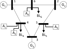
Figure 1: Power system example featuring 6 buses, 3 generators, 4 aggregators, and base loads at three of the buses.

Problem (12) that yields the updated multipliers $\bm{\mu}(k+1)$ and the approximate dual value $D_{\mathrm{ap}}(\bm{\mu}(k+1))$ can be solved at the MO. To this end, the quantities $\{D_{j}(\bm{\mu}(k)),\sum_{r,s}{p}_{jrs}^{t}(k)\}_{j}$ are needed from each aggregator per iteration $k$ as the problem input. Note that $D_{j}(\bm{\mu}(k)):=\sum_{r\in\mathcal{R}_{j}}D_{jr}(\bm{\mu}(k))$, where $D_{jr}(\bm{\mu}(k))$ is the optimal value of problem (7b). Thus, it is clear that all these required quantities can be formed at the aggregator level as summations over all end-users, and then transmitted to the MO. The highlight here is that the proposed decomposition scheme respects user privacy, since $B_{jrs}(\mathbf{p}_{jrs})$ and $\mathcal{P}_{jrs}$ are never revealed.

IV Numerical tests

In this section, simulation results are presented to verify the merits of the disaggregated bundle method. The power system tested for market clearing and large-scale DR is illustrated in Fig. 1, where each of the 4 aggregators serves 1,000 residential end-users. The scheduling horizon starts from 1am until 12am, for a total of 24 hours.

Time-invariant generation cost functions are set to be quadratic as $C_{i}(P_{G_{i}}^{t})=a_{i}(P_{G_{i}}^{t})^{2}+b_{i}P_{G_{i}}^{t}$ for all $i$ and $t$. Each end-user has a PHEV to charge overnight. All detailed parameters of the generators and loads are listed in Tables I and II. The utility functions $\{B_{jrs}(\cdot)\}$ are set to be zero for simplicity. The upper bound on each aggregator’s consumption is $P_{\mathrm{DRA}_{j}}^{\max}=50$ MW while $\mathbf{p}_{\mathrm{BL}}^{t}=5$ MW. At a base of 100 MVA, the values of the network reactances are $\{X_{16},X_{62},X_{25},X_{53},X_{34},X_{41}\}=\{0.2,0.3,0.25,0.1,0.3,0.4\}$ p.u. Finally, no flow limits are imposed across the network. The resulting optimization problems (7a) and (12) are modeled via YALMIP [9], and solved by Gurobi [10].

TABLE I: Generator parameters. The units of $a_{i}$ and $b_{i}$ are $/(MWh)² and $/MWh, respectively. the rest are in MW.

Gen.	$a_{i}$	$b_{i}$	$P_{G_{i}}^{\max}$	$P_{G_{i}}^{\min}$	$\mathsf{R}_{i}^{\mathrm{up,down}}$
1	0.3	3	60	2.4	50
2	0.15	20	50	0	35
3	0.2	50	50	0	40

TABLE II: Parameters of residential appliances. All listed hours are the ending ones; w.p. means with probability.

$E_{\mathrm{PHEV}}$ (kWh)	Uniform on {10, 11, 12}
$p_{\mathrm{PHEV}}^{\max}$ (kWh)	Uniform on {2.1, 2.3, 2.5}
$p_{\mathrm{PHEV}}^{\min}$ (kWh)	0
$T_{jr1}^{\mathrm{st}}$	1am
$T_{jr1}^{\mathrm{end}}$	6am w.p. 70%, 7am w.p. 30%

Figs. 2 and 3 illustrate the convergence performance of the proposed disaggregated bundle method vis-à-vis the disaggregated CPM. The pertinent parameters are set as $\epsilon=10^{-3}$, $\rho(k)\equiv 0$, $\beta=0.5$, and $\bm{\mu}^{\max,\min}=\mathbf{\pm 50}$ (cf. [6]). Fig. 2 depicts the evolution of the objective values of the dual $D(\bm{\mu}(k))$ and the approximate dual $D_{\mathrm{ap}}(\bm{\mu}(k+1))$. It is clearly seen that the bundle method converges much faster (more than three times) than its CPM counterpart. Note that due to the effect of the proximal penalty (cf. (11a)), quantity $D_{\mathrm{ap}}(\bm{\mu}(k+1))$ for the bundle may not always serve as an upper bound of $f^{*}$ as the one for the CPM. Finally, convergence of the Lagrange multiplier sequence $\bm{\mu}(k)$ is shown in Fig. 3, which also corroborates the merit of the bundle method for its faster parameter convergence over the CPM. It is interesting to observe that the distance-to-optimal curve of the bundle method is quite smooth compared with the CPM one. This again illustrates the effect of the proximal regulation penalizing large deviations.

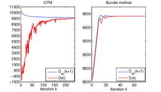
Figure 2: Convergence of the objective values of the dual and the approximated one (denoted as $D(k)$ and $D_{\mathrm{ap}}(k+1)$ in the caption).

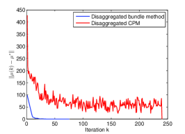
Figure 3: Convergence of the Lagrange multipliers.

V Conclusions and Future Directions

In this work, a fast convergent and scalable distributed solver is developed for market clearing with large-scale residential DR. Leveraging the dual decomposition technique, only the aggregator-users balance constraint is dualized in order to separate problems for the MO and each aggregator, while respecting end-user privacy concerns. Simulated tests highlight the merits of the proposed approach for multiplier updates based on the disaggregated bundle method.

A number of interesting research directions open up, including the incorporation of load and renewable energy production uncertainty, the issue of primal recovery, as well as cut aggregation techniques for further computational speed up.

References

- [1] A. M. Giacomoni, S. M. Amin, and B. F. Wollenberg, “Reconfigurable interdependent infrastructure systems: Advances in distributed sensing, modeling, and control,” in Proc. American Control Conf., San Francisco, CA, June–July 2011.
- [2] C.-L. Su and D. Kirschen, “Quantifying the effect of demand response on electricity markets,” IEEE Trans. Power Systems, vol. 24, no. 3, pp. 1199–1207, Aug. 2009.
- [3] J. Wang, S. Kennedy, and J. Kirtley, “A new wholesale bidding mechanism for enhanced demand response in smart grids,” in Proc. IEEE PES Conf. Innovative Smart Grid Tech., Gaithersburg, MD, Jan. 2010.
- [4] J.-Y. Joo and M. D. Ilić, “Adaptive load management (ALM) in electric power systems,” in Proc. Int. Conf. Networking, Sensing, and Control, Chicago, IL, Apr. 2010, pp. 637–642.
- [5] K. Trangbeak, M. Petersen, J. Bendtsen, and J. Stoustrup, “Exact power constraints in smart grid control,” in Proc. 50th IEEE Conf. Decision and Control and European Control Conf., Orlando, FL, Dec. 2011, pp. 6907–6912.
- [6] N. Gatsis and G. B. Giannakis, “Decomposition algorithms for market clearing with large-scale demand response,” IEEE Trans. Smart Grid, 2013 (to appear).
- [7] D. P. Bertsekas, Convex Optimization Theory. Belmont, MA: Athena Scientific, 2009.
- [8] J. B. Hiriart-Urruty and C. Lemaréchal, Convex Analysis and Minimization Algorithms. Berlin Heidelberg New York: Springer-Verlag, 1993, vol. II.
- [9] J. Löfberg, “YALMIP: A toolbox for modeling and optimization in MATLAB,” in Proceedings of the CACSD Conference, Taipei, Taiwan, 2004. [Online]. Available: http://users.isy.liu.se/johanl/yalmip
- [10] Gurobi Optimization, Inc., “Gurobi optimizer reference manual,” 2013. [Online]. Available: http://www.gurobi.com