Assessment of the 2880 impact threat from asteroid (29075) 1950 DA

Abstract

In this paper we perform an assessment of the 2880 Earth impact risk for asteroid (29075) 1950 DA. To obtain reliable predictions we analyze the contribution of the observational dataset and the astrometric treatment, the numerical error in the long-term integration, and the different accelerations acting on the asteroid. The main source of uncertainty is the Yarkovsky effect, which we statistically model starting from 1950 DA’s available physical characterization, astrometry, and dynamical properties. Before the realease of 2012 radar data, this modeling suggests that 1950 DA has 99% likelihood of being a retrograde rotator. By using a 7-dimensional Monte Carlo sampling we map 1950 DA’s uncertainty region to the 2880 close approach $b$-plane and find a $5\times 10^{-4}$ impact probability. With the recently released 2012 radar observations, the direct rotation is definetly ruled out and the impact probability decreases to $2.5\times 10^{-4}$.

1 Introduction

Near Earth asteroid (29075) 1950 DA was first discovered in 1950 by C. A. Wirtanen at Lick Observatory (Wirtanen and Vasilevskis, 1950) and then lost for more than 50 yr. In December 2000 the asteroid was rediscovered at Lowell Observatory-LONEOS (Bardwell, 2001) as 2000 YK₆₆ and subsequently recognized to be 1950 DA.

In 2001, 1950 DA experienced an Earth close approach at 0.05 au and radar observations were obtained from Arecibo and Goldstone. These radar observations significantly reduced the orbital uncertainty and allowed long-term predictions. In particular, Giorgini et al. (2002) showed that there is a non-negligible probability (upper bound 0.33%) for an Earth impact in March 2880. The occurrence of such an impact is decisively driven by the Yarkovsky effect, a subtle nongravitational perturbation arising from the anisotropic re-emission at thermal wavelengths of absorbed solar radiation. This perturbation causes a secular variation in semimajor axis resulting in a mean anomaly runoff that accumulates quadratically with time (Vokrouhlický et al., 2000). As 1950 DA experiences several planetary encounters (Giorgini et al., 2002, Table 1), the runoff caused by the Yarkovsky effect is amplified and therefore becomes important for 1950 DA’s predictions.

Busch et al. (2007) use the 2001 radar observations to constrain the physical properties of 1950 DA. The Ondrejov Asteroid Photometry Project provides additional information on 1950 DA’s physical model from lightcurve observations obtained during the 2001 close approach. However, the known physical characterization does not yet allow an estimate of the Yarkovsky effect. In particular, the pole orientation is still unknown and so is the sign of 1950 DA’s orbital drift.

Because of the decisive contribution of the Yarkovsky effect, 1950 DA belongs to a class of “special objects”, which also includes asteroids (99942) Apophis (Farnocchia et al., 2013b) and (101955) Bennu (Chesley et al., 2013). Each of these objects presents unique features and demanding tasks. In particular, for 1950 DA we are pushing the impact prediction horizon for a time interval that is four times longer than ever analyzed for any other asteroid. Therefore, performing the impact hazard assessment requires a specific effort and the development of ad hoc techniques beyond what is routinely done by the automatic impact monitoring systems Sentry and NEODyS (Milani et al., 2005a).

2 Orbital solution

1950 DA has a long observed arc that allows a precise estimate of the orbit. The earliest 18 observations are from 1950. Then, we have two isolated observations in 1981 and more than 450 observations from 2000 to 2012. Moreover, in March 2001 the Arecibo and Goldstone observatories obtained 13 radar observations, specifically 8 delay and 5 Doppler measurements (Giorgini et al., 2002). (The contribution of the recently released 2012 radar observations is discussed in Sec. 8.)

To properly handle the observation dataset and mitigate the effect of star catalog systematic errors, we applied the debiasing and weighting described by Chesley et al. (2010), which we refer to as CBM10. Furthermore, for observatories with $N>7$ observations on the same night we relaxed the weights by a factor $\sqrt{N/5}$. This relaxation factor reduces the contribution of batches containing a large number of observations, e.g., Ondrejov lightcurve observations in late February 2001. Among the post-2000 observations, there are batches showing unusually high astrometric biases and therefore we removed all the batches with apparent bias larger than 1”. The discovery observation has a low number of significant digits, so it was weighted at 30”. Finally, we applied weights at 2” to observations marked with the MPC flag ‘A’, i.e., when right ascension and declination in the J2000 system were obtained by rotating the B1950 coordinates. Table 1 contains the orbital elements corresponding to this astrometric treatment, which is referred to as “Nominal” throughout the paper. It is worth pointing out that this solution was computed without accounting for the Yarkovsky effect, which is discussed in Sec.3

Epoch	2012 Sep 30.0	TDB
Eccentricity	0.5082852298(358)
Perihelion distance	0.8350375895(606)	au
Perihelion time	2012 May 8.94652197(622)	TDB
Longitude of ascending node	356.72810476(900)	deg
Argument of perihelion	224.61346319(964)	deg
Inclination	12.17480729(584)	deg

Table 1: Orbital solution for asteroid 1950 DA. Numbers in parentheses indicate the 1$\sigma$ formal uncertainties for the corresponding digits in the parameter value.

Table 2 shows the normalized RMS according to different observational datasets and astrometric schemes: a) observations only from 1950 to March 2001, which is similar to the dataset used by Giorgini et al. (2002) and which we refer to as the G02 dataset; b) G02 with the application of the Chesley et al. (2010) astrometric scheme (G02 + CBM10); c) the full observational dataset with the application of the Chesley et al. (2010) astrometric scheme (ALL + CBM10); d) the full observation dataset and the astrometric treatment described above (Nominal). It is interesting to note that the nominal solution provides the best match to the 2001 delay measurements, which highlights the importance of using the full arc and the goodness of the astrometric scheme described before. The table also contains the coordinates on the 2880 $b$-plane, which is the plane normal to the incoming asymptote of the geocentric hyperbola on which the asteroid travels when it is closest to the planet (Valsecchi et al., 2003). The $\zeta$ axis is in the direction on the $b$-plane opposite to the projection of the velocity of the Earth and the $\xi$ axis completes the right-handed coordinate system. The G02 solution has the largest positive $\zeta_{2880}$, i.e., is the one arriving at the close approach with the largest delay. The Chesley et al. (2010) astrometric scheme and the use of the full arc progressively decrease $\zeta_{2880}$, with the nominal solution reaching the 2880 close approach with the largest advance with respect to the Earth. Our nominal solution is 1.46$\sigma$ away from the G02 prediction, for which $\sigma_{\zeta_{2880}}=3.19\times 10^{6}$ km.

Astrometry	NRMS	$\xi_{2880}$	$\sigma_{\xi_{2880}}$	$\zeta_{2880}$	$\sigma_{\zeta_{2880}}$
	in delay	[$10^{3}$ km]	[km]	[$10^{6}$ km]	[$10^{6}$ km]
G02	0.731	22.8	5.08	2.65	3.19
G02 + CBM10	0.728	0.88	4.55	0.61	3.19
All + CBM10	0.719	5.25	3.41	-1.32	1.61
Nominal	0.706	11.8	3.56	-2.01	1.65

Table 2: Normalized RMS (NRMS) for the 2001 radar delay measurements and $b$-plane coordinates for different observation datasets and astrometric schemes.

Figure 1 shows the uncertainty region on the 2880 $b$-plane. The 1$\sigma$ semi-width of the uncertainty region is 3–4 km, e.g., for $\zeta_{2880}=0$ the full width is 7.12 km. Therefore, we can perform the risk assessment by using a one dimensional analysis. In particular, we consider the Line of Variation (LOV, Milani et al., 2005b), i.e., the line along which the uncertainty region is most stretched and is therefore representative of the orbital uncertainty. The nonlinearity of the mapping from the orbital uncertainty space to the $b$-plane is evident from the curvature of the uncertainty region and the locations of the $\sigma$ levels. The Earth is at 1.64$\sigma$ from the nominal solution and a simplistic computation of the corresponding impact probability (IP) is 5.06 $\times$ 10^-4. However, the computation of a reliable IP requires a more careful analysis as discussed in the following sections.

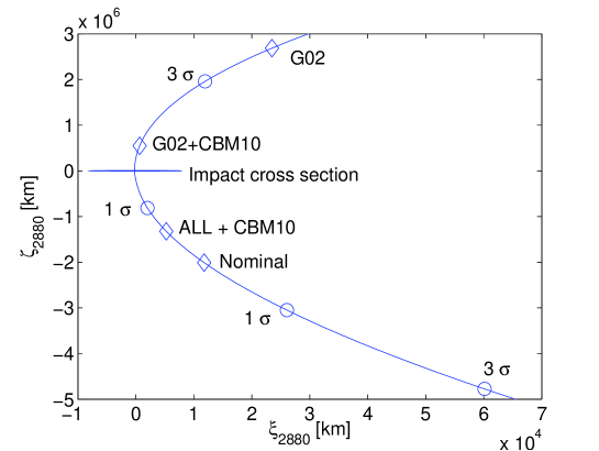
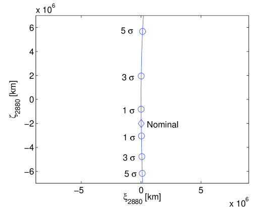
Figure 1: Line of variation in the 2880 $b$-plane. In the left panel diamonds are the $b$-plane coordinates of the orbital solutions corresponding to different observation datasets and astrometric schemes as described in Table 2. Circles are 1, 3, and 5$\sigma$ levels with respect to the nominal solution. The impact cross section has radius 1.24 Earth radii. The right panel shows the LOV and the $\sigma$ levels using the same scale for the axes.

3 Nongravitational perturbations

Nongravitational perturbations can play an important role for long term predictions, therefore we used the following comet-like model (Marsden et al., 1973):

$$\mathbf{a}_{NG}=\left(\frac{r_{0}}{r}\right)^{2}\left(A_{1}\hat{\mathbf{r}}+A_{2}\hat{\mathbf{t}}\right)$$ (1)

where $r_{0}=1$ au, $r$ is the heliocentric distance of the asteroid, $\hat{\mathbf{r}}$ is the radial direction, and $\hat{\mathbf{t}}$ is the transverse direction.

The radial component of $\mathbf{a}_{NG}$ models direct and reflected solar radiation pressure and $A_{1}$ can be related to the asteroid’s physical quantities as follows (Vokrouhlický and Milani, 2000):

$$A_{1}=\left(1+\frac{4}{9}A\right)AMR\frac{G_{S}}{c}$$ (2)

where $A$ is the Bond albedo, $AMR$ is the asteroid’s area-to-mass ratio, $G_{S}=1371$ W/m² is the solar constant, and $c$ is the speed of light.

The transverse component of $\mathbf{a}_{NG}$ models the Yarkovsky perturbation (Bottke et al., 2006) and $A_{2}$ can be related to the asteroid’s physical quantities as follows (Farnocchia et al., 2013a):

$$A_{2}=\frac{4(1-A)}{9}\Phi(1\mbox{au})f(\Theta)\cos\gamma\;,\ \ f(\Theta)=\frac{0.5\Theta}{1+\Theta+0.5\Theta^{2}}$$ (3)

where $\Phi(1\mbox{au})$ is the standard radiation force factor at 1 au, $\Theta$ is the thermal parameter, and $\gamma$ is the obliquity (Vokrouhlický et al., 2000). To drop the dependence of $\Theta$ on $r$, we computed the subsolar temperature (Vokrouhlický, 1998) at the orbital semilatus rectum.

3.1 Physical model

Though $A_{1}$ and $A_{2}$ are unknown, we can generate a statistical sample representing these two parameters starting from the available information on 1950 DA’s physical model. Table 3 reports the known physical parameters from Busch et al. (2007) and the Ondrejov Asteroid Photometry Project. In particular, Busch et al. (2007) provide two models for 1950 DA’s rotation state, i.e., direct and retrograde. As a result, the following analysis initially discusses these two models separately, unifying them only in the next subsection. Note that the spin orientations found by Busch et al. (2007) correspond to an obliquity of 24.5^∘ (for the direct model) and 167.7^∘ (for the retrograde model). Therefore, the spin axis is far from being in the orbital plane and the seasonal component of the Yarkovsky effect can be neglected.

	Direct rotation	Retrograde rotation
Spin $(\lambda,\beta)\pm 5^{\circ}$	$(88.6^{\circ},77.7^{\circ})$	$(187.4^{\circ},-89.5^{\circ})$
Effective diameter $D$ $\pm$ 10%	1.16 km	1.30 km
Minimum bulk density $\rho_{\min}$ $\pm$ 10%	3.0 g/cm3	3.5 g/cm3
Absolute magnitude $H$	17.55 $\pm$ 0.3
Slope parameter $G$	0.03 $\pm$ 0.1
Rotation period $P_{rot}$	2.12160 $\pm$ 0.00004 h

Table 3: Available physical characterization of 1950 DA. $\lambda$, $\beta$, $D$, and $\rho_{\min}$ are from Busch et al. (2007), $H$, $G$, and $P_{rot}$ from the Ondrejov Asteroid Photometry Project.

Figure 2 shows the geometric albedo $p_{V}$ distribution, which was obtained from the absolute magnitude $H$ and equivalent diameter $D$ according to Pravec and Harris (2007):

$$D=1329\ \frac{10^{-0.2H}}{\sqrt{p_{V}}}\,.$$ (4)

The albedo distribution depicted in Fig. 2 is lower than the geometric albedo reported by Busch et al. (2007), i.e., $p_{V}$ from 0.20 to 0.25. The reason for this difference is solely due to different estimates of $H$. Indeed, Busch et al. (2007) use photometry information from 125 optical observations and obtain $H=16.8$. However, Jurić et al. (2002) show the presence of biases in the known asteroid absolute magnitudes catalog. Therefore, we preferred to use the absolute magnitude reported by the Ondrejov Asteroid Photometry Project, i.e., $H=$17.55 $\pm$ 0.3. This value of $H$ also appears to be more consistent with the 0.07 $\pm$ 0.02 geometric albedo reported by NEOWISE (Mainzer et al., 2011).

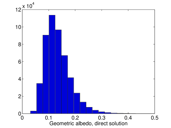
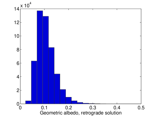
Figure 2: Albedo distribution for both the direct and the retrograde models obtained by using the diameter from Busch et al. (2007) and the absolute magnitude from the Ondrejov Asteroid Photometry Project.

Rivkin et al. (2005) suggest an EM taxonomic classification for 1950 DA. From the JPL Small Body Database we obtain that the typical geometric albedo for E type asteroids is $\sim$ 0.4, therefore the taxonomic type M (typical geometric albedo $\sim$ 0.17) seems more likely. By selecting M type asteroids from Carry (2012), we obtain an average bulk density $\rho=3.86\pm 0.87$ g/cm³. Moreover, Busch et al. (2007) report a minimum bulk density (see Table 3). Therefore, we used a truncated normal distribution for $\rho$.

Delbò et al. (2007) give a relationship between thermal inertia $\Gamma$ and diameter $D$ (in km):

$$\Gamma=d_{0}D^{-\psi}\ ,d_{0}=(300\pm 45)\mbox{ J m${}^{-2}$ s${}^{-0.5}$ K${}^{-1}$}\ ,\ \psi=0.36\pm 0.09\ .$$

A preliminary thermal model of 1950 DA obtained from NEOWISE data appears to be consistent with this relationship (Nugent et al., 2013). From $\Gamma$ and the $P_{rot}$ (see Table 3) we computed the thermal parameter $\Theta$ according to Vokrouhlický (1998).

By using Eq. (2) and Eq. (3) we can map the physical parameters described in this section and their uncertainties to the nongravitational parameters $A_{1}$ and $A_{2}$. We then obtain the distributions of Fig. 3 and Fig. 4 for the direct and retrograde models.

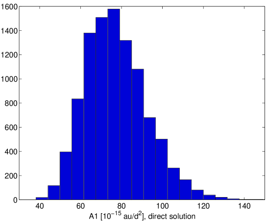
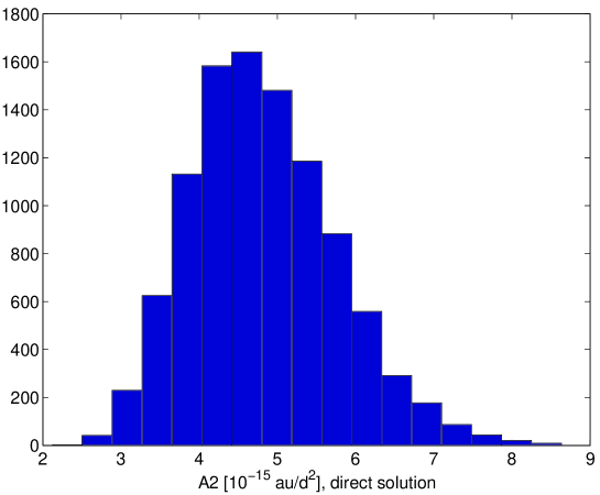
Figure 3: Nongravitational parameters sampling for the direct model.

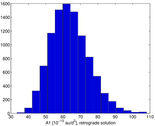
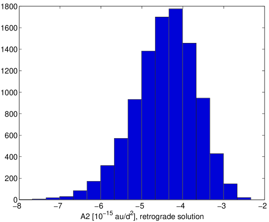
Figure 4: Nongravitational parameters sampling for the retrograde model.

3.2 Overall distribution of the Yarkovsky effect

The physical model provides us with two possible distributions for the Yarkovsky parameter $A_{2}$. To obtain a single distribution of $A_{2}$ we can use the following pieces of information from the following sources:

• According to Busch et al. (2007), both the direct and retrograde physical models provide good fits to radar and lightcurve data. Therefore, 1950 DA has a 50% probability of being direct and a 50% probability of being retrograde.

• The astrometry provides an additional constraint. In fact, if we solve for $A_{2}$ in the orbital fit to the observations (Farnocchia et al., 2013a), we find $A_{2}=(-4.94\pm 3.71)$ $\times$ 10^-15 au/d², which favors a retrograde rotation.

• The dynamical history of 1950 DA provides additional information. In fact, by using the Bottke et al. (2002) Near Earth Object population model, we have that 1950 DA has a 63% probability of coming from the $\nu_{6}$ resonance (Bottke, personal communication). As $\nu_{6}$ is at the inner edge of the Main Belt region, such objects can generally enter only by drifting inwards due to retrograde rotation. For the other NEO source regions we assume equal probability of entering by drifting inwards or outwards (La Spina et al., 2004). Therefore, the probabilities that 1950 DA is direct or retrograde are 81.8% and 18.2%, respectively.

These are independent sources of information that can be used to obtain the overall distribution of $A_{2}$. Figure 5 shows how the distribution of $A_{2}$ changes when the different pieces of information are sequentially added. The distribution labeled with P only uses the information from the physical model (i.e., 50%-50% retrograde-direct ratio), PA uses also the astrometry. Finally, PAD uses all the information above and is therefore the one we consider most reliable. Negative values of $A_{2}$ are predominant thus suggesting that 1950 DA is likely to be a retrograde rotator with a probability of 99%. As a further confirmation, the geometric albedo reported by NEOWISE is 0.07 $\pm$ 0.02, which somewhat favors the retrograde solution (see Fig. 2).

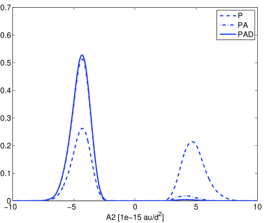
Figure 5: Distribution of $A_{2}$ obtained by using the physical model only (P), physical model plus astrometry (PA), and physical model plus astrometry plus dynamics (PAD).

4 Integration error

The numerical integration produces a numerical error that can be relevant for a long-term propagation. At each integration step we introduce a random error below a fixed integration tolerance, which we set to 10^-15. To estimate the numerical error in the propagation through 2880 we compared the integration in double precision (which is our default) to that in quadruple precision, assumed as the truth. We made this comparison for 121 virtual asteroids (VAs) on the LOV: each VA was propagated from the orbital solution epoch to 2880 in both double and quadruple precision. Figure 6 shows the distribution of the integration error in the logarithmic scale. The integration error has a mean of $\sim$ 15000 km, but can be as large as $\sim$ 150000 km.

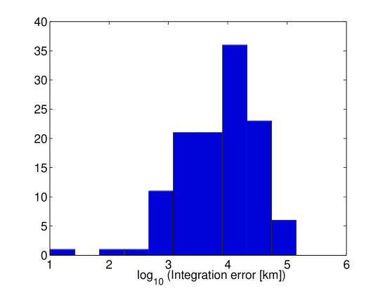
Figure 6: Distribution of the integration error from 2012 to 2880 for 121 virtual orbits along the LOV. The mean is $\sim$ 15000 km.

5 Dynamical error budget

The long-term propagation through 2880 requires an assessment of the relevance of the various perturbations affecting the dynamics of 1950 DA. Our dynamical model included:

• the Newtonian attraction of the Sun, eight planets, Pluto, and the Moon based on JPL’s DE424 planetary ephemerides (Folkner, 2011);

• the Einstein-Infeld-Hoffman (EIH) relativistic approximation (Moyer, 2003) for the Sun, the planets, and the Moon;

• the second order harmonics of the Earth gravity field for geocentric distance $<$ 0.01 au;

• the Newtonian attraction of the 16 most massive asteroids “BIG-16” (e.g., see Table 1 in Farnocchia et al., 2013b).

Figure 7 and Table 4 show the shift in the 2880 $b$-plane coordinates for different settings of the dynamical model. For each setting, we computed a corresponding best-fitting orbital solution and propagated through 2880 to obtain the $b$-plane shift with respect to the nominal prediction, which corresponds to $A_{1}=0$ au/d² and $A_{2}=0$ au/d².

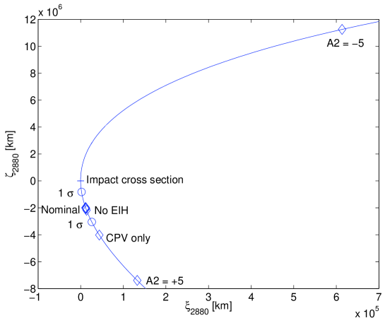
Figure 7: Coordinates on the $b$-plane for different settings of the dynamical model.

	$\Delta\xi_{2880}$ [km]	$\Delta\zeta_{2880}$ [$10^{4}$ km]
Sun only relativity (No EIH)	2030	-17.4
Earth obl. (cut-off at 1 au)	34.3	-0.30
CPV only	32100	-202
BIG-16 + (78) Diana	131	1.17
BIG-16 + 9 pert. Bennu	704	-6.20
$m_{\Mercury}$ +(-) 1$\sigma$	-19.6 (159)	0.17 (-1.41)
$m_{\Venus}$ +(-) 1$\sigma$	161 (-177)	-1.43 (1.58)
$m_{\Earth}$ +(-) 1$\sigma$	-30.7 (-199)	0.27 (1.78)
$m_{\Mars}$ +(-) 1$\sigma$	506 (309)	-4.46 (-2.74)
$m_{\Jupiter}$ +(-) 1$\sigma$	-36.2 (-212)	0.32 (1.90)
$m_{\Saturn}$ +(-) 1$\sigma$	-174 (-170)	1.55 (1.52)
$m_{\Uranus}$ +(-) 1$\sigma$	-77.9 (133)	0.69 (-1.18)
$m_{\Neptune}$ +(-) 1$\sigma$	203 (-156)	-1.80 (1.39)
$m_{\Pluto}$ +(-) 1$\sigma$	-201 (-136)	1.80 (1.21)
$m_{\Moon}$ +(-) 1$\sigma$	-135 (-145)	1.20 (1.30)
$A_{1}$ = 7 $\times$ 10-14 au/d2	-118	1.05
$A_{2}$ = 5 $\times$ 10-15 au/d2	120846	-537
$A_{2}$ = -5 $\times$ 10-15 au/d2	601720	1327

Table 4: Displacement of target plane coordinates for different dynamical settings.

Among gravitational perturbations, the use of Ceres, Pallas, and Vesta only (CPV) as perturbing asteroid produces a very large error. On the other hand other perturbers such as (78) Diana, indicated by Giorgini et al. (2002) as the perturbing asteroid experiencing the closest approach to 1950 DA, and the nine additional asteroids considered by Chesley et al. (2013) for Bennu have a smaller contribution. The 1$\sigma$ variation of planetary masses and the Moon is rather small and dominated by the integration error. Using 0.01 au as a cut-off for including the Earth oblateness effect is a good approximation. In fact, increasing the cut-off to 1 au has a negligible effect. On the other hand, the use of a Sun-only relativistic model produces a significant shift with respect to the nominal prediction.

For nongravitational perturbations, solar radiation pressure has a negligible effect. This small effect can be explained by the fact that the orbital fit to the observations corrects the semimajor axis to compensate for the reduced gravitational parameter of the Sun $GM^{\prime}_{\odot}=GM_{\odot}(1-A_{1}r_{0}^{2}/GM_{\odot})$, where $G$ is the gravitational constant and $M_{\odot}$ is the mass of the Sun. Thus, changing $A_{1}$ alters the semimajor axis but not the orbital period. The Yarkovsky effect has the largest effect and is the main source of uncertainty for the 2880 $b$-plane prediction. For retrograde rotation, i.e., $A_{2}<0$, we have that $\zeta_{2880}$ increases. This behavior is counterintuitive, as a negative orbital drift should imply a smaller period and thus an earlier arrival to the 2880 close approach. However, Fig. 8 shows how Earth approaches before 2880 can flip the uncertainty region and cause this unexpected phenomena. It is important to note that to move the nominal solution toward the Earth we need a retrograde rotation. Therefore, the impact is much more likely with a retrograde rotation, which is the opposite of the result obtained by Giorgini et al. (2002) and is due to the different sign of $\zeta_{2880}$ for the two solutions (see Fig. 1)

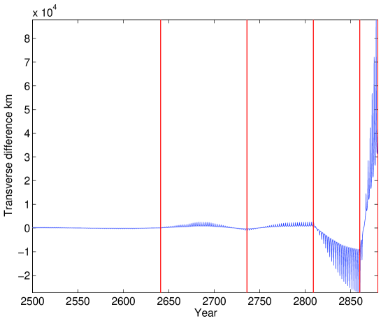
Figure 8: Along-track difference between a propagation with $A_{2}=5$ $\times$ 10^-15 au/d² and a propagation without the Yarkovsky perturbation in the dynamical model. The vertical lines correspond to Earth close approaches with geocentric distance smaller than 0.1 au.

We did not consider other perturbations, such as Galactic tide, Solar mass loss, or Solar oblateness, as Giorgini et al. (2002) demonstrate that the contribution of these perturbations is small and can be neglected.

6 Risk assessment

The impact risk assessment can be performed by means of a Monte Carlo simulation. First, we randomly sampled $A_{2}$ according to the distributions of Fig. 5. Then, for each value of $A_{2}$ we computed the best fitting orbital solution by using our nominal astrometric treatment and randomly selected a VA according to the orbital covariance matrix. Finally, we propagated the VA onto the 2880 $b$-plane.

Figure 9 shows the distribution of $\zeta_{2880}$ corresponding to the P, PA, and PAD distributions of Fig. 5. The peaks on the left are related to the direct solution for the rotation state and therefore the height decreases when more constraints on $A_{2}$ are added and the retrograde solution becomes more likely. On the other hand the peaks on the right correspond to the retrograde solution.

The probability of an impact (IP) can be computed by multiplying the $\zeta_{2880}$ probability density function (PDF) and the width $w$ of the intersection between the LOV and the impact cross section. Note that $w=15856$ km, which is somewhat smaller than the diameter of the impact cross section as the LOV does not pass directly through the center of the Earth ($\xi_{2880}=-234$ km for $\zeta_{2880}=0$). The best estimate of the IP is 4.69 $\times$ 10^-4, which is given by the PAD solution. The corresponding Palermo Scale (Chesley et al., 2002) is $-0.56$.

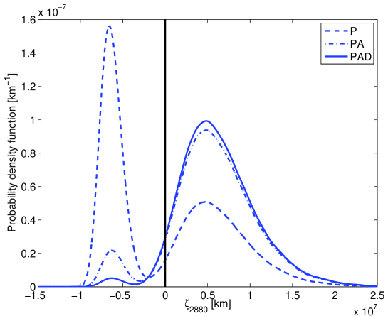
Figure 9: Probability density function of $\zeta_{2880}$ corresponding to the P, PA, and PAD distributions of Fig. 5. The vertical bar marks the location of the impact cross section of the Earth.

As reported by Table 5 the IP is not very sensitive to the amount of information used to constrain $A_{2}$. Furthermore, Table 5 shows the dependence of the IP on the assumptions on 1950 DA’s physical model. The IP always has a similar order of magnitude, thus giving robustness to our result.

	IP [$10^{-4}$]
PAD	4.69
P	2.53
PA	4.44
$H=16.8$ $\pm$ 0.3 as in Busch et al. (2007)	5.73
$H=17.1$ $\pm$ 0.3 from MPC	5.20
$G=0.15\pm 0.1$	4.95
$D=1.5$ km $\pm$ 10%	6.74
$D=0.8$ km $\pm$ 10%	1.20
$d_{0}=200$ $\pm$ 45 J m-2 s-0.5 K-1	1.64
$d_{0}=400$ $\pm$ 45 J m-2 s-0.5 K-1	9.11
$\rho=2.5\pm 0.87$ g/cm3	1.03
$\rho=4.5\pm 0.87$ g/cm3	5.91

Table 5: Impact probability for different constraints on the Yarkovsky effect and different assumptions on the physical parameters of 1950 DA defined in Sec.3.1.

7 Conclusions

We found a $5\times 10^{-4}$ probability for an Earth impact of asteroid (29075) 1950 DA in March 2880. The corresponding Palermo Scale is $-0.56$, which is the highest among known possible asteroid impacts. The long-term propagation calls for a detailed analysis of all the possible sources of error, such as the astrometric treatment, the dynamical model, and the integration error. Due to the related secular variation in semimajor axis, the Yarkovsky effect plays a decisive role in the risk assessment. Even though the Yarkovsky perturbation can be modeled from the available physical characterization of 1950 DA, there is ambiguity in the rotation state and therefore in the sign of the Yarkovsky related orbital drift. To deal with this problem we introduced two additional constraints related to the fit to the astrometric data and the dynamical history of 1950 DA. Both these constraints suggest that the retrograde rotation is more likely, with an overall $\sim$99% probability. We combined these two new independent sources of information with the physical model to enhance our knowledge of the Yarkovsky effect, which was in turn used to compute the probability of an impact in 2880. The exceptional effort required to assess the impact threat from 1950 DA outlines the importance of the impact monitoring as part of the near-Earth asteroids tracking and risk mitigation. Future radar opportunities such as the 2032 close approach should confirm the spin orientation and better estimate the Yarkovsky effect, thus resulting in an improved risk assessment.

8 Update

After the paper was accepted, the 2001 radar observations were remeasured and two 2012 Arecibo range measurement were released (Busch et al., 2013). With the new data the astrometry provides a much stronger constraint to the Yarkovsky effect, i.e., $A_{2}=(-6.70\pm 1.29)\times 10^{-15}$ au/d², and confirms that 1950 DA is a retrograde rotator.

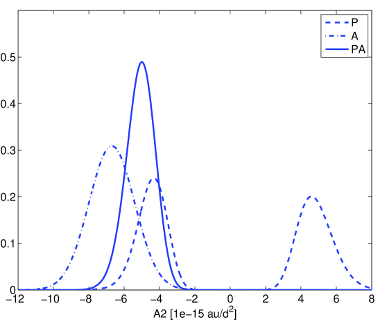
Figure 10: Updated distribution of $A_{2}$ obtained by using the physical model only (P), the astrometry only (A), and a combination of physical model and astrometry (PA).

Figure 10 is an update of Fig. 5. We consider the constraints from either the physical model (P) or the astrometry (A), as well as the combination of them (PA). The constraint from the dynamical evolution of 1950 DA is not present as the astrometry already rules out the direct rotation. By using the same technique described in Sec. 6 we can compute the corresponding impact probabilities: $4.44\times 10^{-4}$ for P, $5.05\times 10^{-5}$ for A, and $2.48\times 10^{-4}$ for PA.

On one hand the astrometry suggests that the physical model is underestimating the size of the Yarkovsky effect. A possible explanation could be the presence of cohesive forces (Scheeres et al., 2010), which would lower the minimum bulk density. Another possibility is that the thermal inertia of 1950 DA is between 50 and 250 J m^-2 s^-0.5 K^-1, which is smaller than Delbò et al. (2007) suggest but would still make sense as the known NEA thermal inertias are quite scattered. On the other hand, the physical model suggests that $A_{2}$ is on the right side of the distribution obtained by the astrometry. Therefore, we think that using both the astrometry and the physical model (PA) still provides the most reliable solution. The corresponding impact probability is $2.48\times 10^{-4}$ and the Palermo Scale -0.83.

References

- Bardwell (2001) Bardwell, C. M. 2001. Minor Planet Electronic Circulars, 2001-A26.
- Bottke et al. (2002) Bottke, W. F., Morbidelli, A., Jedicke, R., Petit, J.-M., Levison, H. F., Michel, P., Metcalfe, T. S. 2002. Debiased Orbital and Absolute Magnitude Distribution of the Near-Earth Objects. Icarus 156, 399-433.
- Bottke et al. (2006) Bottke, W. F., Vokrouhlický, D., Rubincam, D. P., Nesvorný, D. 2006. The Yarkovsky and Yorp Effects: Implications for Asteroid Dynamics. Annual Review of Earth and Planetary Sciences 34, 157-191.
- Busch et al. (2007) Busch, M. W., and 15 colleagues 2007. Physical modeling of near-Earth Asteroid (29075) 1950 DA. Icarus 190, 608-621.
- Busch et al. (2013) Busch, M. W., Giorgini, J. D., Nolan, M. C., Taylor, P. A. 2013. http://ssd.jpl.nasa.gov/?radar
- Carry (2012) Carry, B. 2012. Density of asteroids. Planetary and Space Science 73, 98-118.
- Chesley et al. (2002) Chesley, S. R., Chodas, P. W., Milani, A., Valsecchi, G. B., Yeomans, D. K. 2002. Quantifying the Risk Posed by Potential Earth Impacts. Icarus 159, 423-432.
- Chesley et al. (2010) Chesley, S. R., Baer, J., Monet, D. G. 2010. Treatment of star catalog biases in asteroid astrometric observations. Icarus 210, 158-181.
- Chesley et al. (2013) Chesley, S. R., and 19 colleagues 2013. Orbit and Bulk Density of the OSIRIS-REx Target Asteroid (101955) Bennu. Submitted to Icarus.
- Delbò et al. (2007) Delbò, M., Dell’Oro, A., Harris, A. W., Mottola, S., Mueller, M. 2007. Thermal inertia of near-Earth asteroids and implications for the magnitude of the Yarkovsky effect. Icarus 190, 236-249.
- Farnocchia et al. (2013a) Farnocchia, D., Chesley, S. R., Vokrouhlický, D., Milani, A., Spoto, F., Bottke, W. F. 2013. Near Earth Asteroids with measurable Yarkovsky effect. Icarus 224, 1-13.
- Farnocchia et al. (2013b) Farnocchia, D., Chesley, S. R., Chodas, P. W., Micheli, M., Tholen, D. J., Milani, A., Elliott, G. T., Bernardi, F. 2013. Yarkovsky-driven impact risk analysis for asteroid (99942) Apophis. Icarus 224, 192-200.
- Folkner (2011) Folkner, M. K. 2011. Planetary Ephemeris DE424 for Mars Science Laboratory Early Cruise Navigation. JPL IOM 343R-11-003.
- Giorgini et al. (2002) Giorgini, J. D., and 13 colleagues 2002. Asteroid 1950 DA’s Encounter with Earth in 2880: Physical Limits of Collision Probability Prediction. Science 296, 132-136.
- Jurić et al. (2002) Jurić, M., and 15 colleagues 2002. Comparison of Positions and Magnitudes of Asteroids Observed in the Sloan Digital Sky Survey with Those Predicted for Known Asteroids. The Astronomical Journal 124, 1776-1787.
- La Spina et al. (2004) La Spina, A., Paolicchi, P., Kryszczyńska, A., Pravec, P. 2004. Retrograde spins of near-Earth asteroids from the Yarkovsky effect. Nature 428, 400-401.
- Mainzer et al. (2011) Mainzer, A., and 36 colleagues 2011. NEOWISE Observations of Near-Earth Objects: Preliminary Results. The Astrophysical Journal 743, 156.
- Marsden et al. (1973) Marsden, B. G., Sekanina, Z., Yeomans, D. K. 1973. Comets and nongravitational forces. V. The Astronomical Journal 78, 211.
- Milani et al. (2005a) Milani, A., Chesley, S. R., Sansaturio, M. E., Tommei, G., Valsecchi, G. B. 2005. Nonlinear impact monitoring: line of variation searches for impactors. Icarus 173, 362-384.
- Milani et al. (2005b) Milani, A., Sansaturio, M. E., Tommei, G., Arratia, O., Chesley, S. R. 2005. Multiple solutions for asteroid orbits: Computational procedure and applications. Astronomy and Astrophysics 431, 729-746.
- Moyer (2003) Moyer, T. D. 2003. Formulation for Observed and Computed Values of Deep Space Network Data Types for Navigation. Wiley-Interscience, Hoboken, NJ.
- Nugent et al. (2013) Nugent, C. R., Mainzer, A., Masiero, J. R., Grav. T., Bauer, J. M. 2013. A new program to determine asteroid thermal properties. IAA Planetary Defense Conference 3, #03.19.
- Pravec and Harris (2007) Pravec, P., Harris, A. W. 2007. Binary asteroid population. 1. Angular momentum content. Icarus 190, 250-259.
- Rivkin et al. (2005) Rivkin, A. S., Binzel, R. P., Bus, S. J. 2005. Constraining near-Earth object albedos using near-infrared spectroscopy. Icarus 175, 175-180.
- Scheeres et al. (2010) Scheeres, D. J., Hartzell, C. M., Sánchez, P., Swift, M. 2010. Scaling forces to asteroid surfaces: The role of cohesion. Icarus 210, 968-984.
- Valsecchi et al. (2003) Valsecchi, G. B., Milani, A., Gronchi, G. F., Chesley, S. R. 2003. Resonant returns to close approaches: Analytical theory. Astronomy and Astrophysics 408, 1179-1196.
- Vokrouhlický (1998) Vokrouhlicky, D. 1998. Diurnal Yarkovsky effect as a source of mobility of meter-sized asteroidal fragments. I. Linear theory. Astronomy and Astrophysics 335, 1093-1100.
- Vokrouhlický and Milani (2000) Vokrouhlický, D., Milani, A. 2000. Direct solar radiation pressure on the orbits of small near-Earth asteroids: observable effects?. Astronomy and Astrophysics 362, 746-755.
- Vokrouhlický et al. (2000) Vokrouhlický, D., Milani, A., Chesley, S. R. 2000. Yarkovsky Effect on Small Near-Earth Asteroids: Mathematical Formulation and Examples. Icarus 148, 118-138.
- Wirtanen and Vasilevskis (1950) Wirtanen, C. A., Vasilevskis, S. 1950. Observations of Minor Planets Made at Lick Observatory. Minor Planet Circulars 416, 1.