Period-luminosity relations in evolved red giants explained by solar-like oscillations

Abstract

Context. Solar-like oscillations in red giants have been investigated with the space-borne missions CoRoT and Kepler, while pulsations in more evolved M giants have been studied with ground-based microlensing surveys. After 3.1 years of observation with Kepler, it is now possible to link these different observations of semi-regular variables.

Aims. We aim to identify period-luminosity sequences in evolved red giants identified as semi-regular variables and to interpret them in terms of solar-like oscillations. Then, we investigate the consequences of the comparison of ground-based and space-borne observations.

Methods. We first measured global oscillation parameters of evolved red giants observed with Kepler with the envelope autocorrelation function method. We then used an extended form of the universal red giant oscillation pattern, extrapolated to very low frequency, to fully identify their oscillations. The comparison with ground-based results was then used to express the period-luminosity relation as a relation between the large frequency separation and the stellar luminosity.

Results. From the link between red giant oscillations observed by Kepler and period-luminosity sequences, we have identified these relations in evolved red giants as radial and non-radial solar-like oscillations. We were able to expand scaling relations at very low frequency (periods as long as 100 days and large frequency separation less than 0.05 $\mu$Hz). This helped us identify the different sequences of period-luminosity relations, and allowed us to propose a calibration of the K magnitude with the observed large frequency separation.

Conclusions. Interpreting period-luminosity relations in red giants in terms of solar-like oscillations allows us to investigate the time series obtained from ground-based microlensing surveys with a firm physical basis. This can be done with an analytical expression that describes the low-frequency oscillation spectra. The different behavior of oscillations at low frequency, with frequency separations scaling only approximately with the square root of the mean stellar density, can be used to precisely address the physics of the semi-regular variables. This will allow improved distance measurements and opens the way to extragalactic asteroseismology with the observations of M giants in the Magellanic Clouds.

1 Introduction

The space-borne missions CoRoT and Kepler have provided many observations and carried out important results, depicting oscillations in red giants as solar-like (De Ridder et al. 2009; Bedding et al. 2010). The oscillation spectra are understood well, including the coupling of waves sounding the core (Beck et al. 2011; Bedding et al. 2011; Mosser et al. 2011a, 2012c) or the effects of rotation (Beck et al. 2012; Deheuvels et al. 2012; Mosser et al. 2012b; Goupil et al. 2013; Marques et al. 2013). These results mostly concern red giants on the low red giant branch (RGB) and on the red clump.

From the ground, microlensing surveys such as MACHO or OGLE have provided a wealth of information on the pulsations observed in M giants (e.g., Wood et al. 1999; Wray et al. 2004; Soszyński et al. 2007; Tabur et al. 2010; Soszyński & Wood 2013, and references therein). These M giants have larger radii than the ones observed with Kepler. The nature of their pulsations has been questioned for some time. There is a fundamental question whether they are self-excited pulsations or stochastically excited modes (Dziembowski et al. 2001; Christensen-Dalsgaard et al. 2001). Evidence of the link between the observed pulsations in M giants and the solar-like oscillations detected in the K giants has been found (Dziembowski & Soszyński 2010, hereafter DS10). Tabur et al. (2010) state that the M giants with the shortest periods bridge the gap between G and K giant solar-like oscillations and M-giant pulsations, revealing a smooth continuity on the giant sequence. We intend to reexamine this question in detail with Kepler data, for instance, through examining the scaling relations governing global seismic parameters.

For red giants, most of the results of the microlensing surveys are expressed as period-luminosity (PL) relations found for different sequences (e.g., Soszyński et al. 2007, hereafter S07). Recently, Takayama et al. (2013) have compared observed period ratios to modeled values; they found close agreement that allows them to identify PL sequences. With long time series recorded by Kepler, we can now also investigate the PL relations of pulsating M giants using these data and compare them with solar-like oscillations. Another puzzling question concerns the degree of the observed pulsation: radial, non-radial, or both? Again, Kepler data may provide useful insights and methods developed for weighting the relative contributions of the different angular degrees and measuring the mode visibility (Mosser et al. 2012a) can be extrapolated for M giants.

In this work, we aim to analyze oscillations at very low frequency, with large frequency separations as low as 0.1 $\mu$Hz, corresponding to pulsations with periods up to 100 days. We intend to extrapolate the results previously obtained for less-evolved RGB stars to the low-frequency domain where M giants oscillate. In Section 2, we present Kepler data that are used and the tools for analyzing them. A similar presentation of the current status of OGLE small amplitude red giants (OSARG) is done in Section 3. In Section 4, different scaling relations of global oscillation parameters are used to verify that oscillations at very low frequency behave like solar-like oscillations. For fully identifying the oscillations, we need to extrapolate the findings of Mosser et al. (2011b), who have proposed a method providing an analytical description of the red giant oscillation pattern, based on homology consideration. The method presented in Section 5 allows us, for the first time, to identify the radial order and the angular degree of solar-like oscillations in M giants. In Section 6, we show how the low-frequency oscillation pattern coincides with PL sequences. This allows a precise physical interpretation, as well as a precise calibration of the PL relation (Section 7). In Section 8, we reanalyze previous results with the new findings. We also investigate the possibility of enhancing the accuracy of distance measurements using solar-like oscillations in giants.

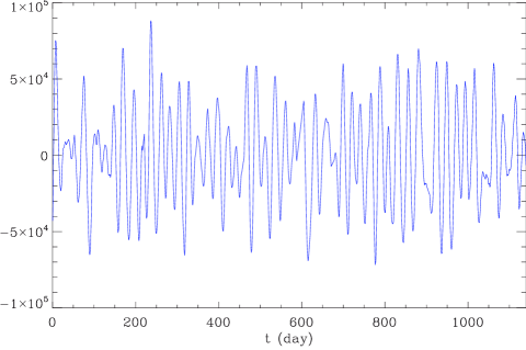
Figure 1: Typical time series of the relative photometric variation of an evolved red giant observed by Kepler (KIC 2831290). The relative amplitude is expressed in ppm.

2 Kepler data and analysis

2.1 Kepler data

We used Kepler long-cadence data recorded up to and including the Kepler observing run Q13, which correspond to the targets considered by the Kepler red giant working group (see, e.g., Bedding et al. 2010). The 38-month-long observation time span provides a frequency resolution of about 10 nHz. Compared to previous work on Kepler red giants, the time series benefited from a refined treatment. The light curves have been extracted from the pixel data, following the methods and corrections described in García et al. (2011) and in Bloemen et al. (2013, in preparation). In a large number of times series, this dedicated treatment provides evidence of large irregular low-frequency variations. It then allows the investigation of oscillations of stars on the upper RGB and on the AGB. Contrary to microlensing studies that deliver a limited number of periods, often only one (e.g., Fraser et al. 2005), up to three (e.g., Takayama et al. 2013, hereafter T13), or up to four (e.g., Tabur et al. 2010), we aim to analyze all peaks that can be identified as reliable in a Fourier spectrum which is free of any aliasing effect.

2.2 Analysis with the envelope autocorrelation function

We used the envelope autocorrelation function (Mosser & Appourchaux 2009) to measure the observed large separation. The method is efficient at low frequency: the envelope autocorrelation function (EACF) corresponds to the autocorrelation of the time series (Fig. 1), with a clear signal at very low frequency, despite a low response due to the small number of frequency bins in the frequency range where the oscillation signal is seen. The precision is, however, limited by the small number of observable modes and the relatively poor frequency resolution. Simulations indicate a relative uncertainty of 5 % for large frequency separation of 0.1 $\mu$Hz measured with the EACF method (compared to less than 1 % at the clump where $\Delta\nu_{\mathrm{obs}}\simeq 4\,\mu$Hz).

Because it benefits from the long time series, almost all 1444 stars of our red giant list exhibit solar-like oscillations. The few with no clear signal have too long periods, or too dim magnitudes, or have complex spectra due to binarity (e.g., Gaulme et al. 2013). We chose to restrict the study to stars with large frequency separations below 2.5 $\mu$Hz, corresponding to a frequency $\nu_{\mathrm{max}}$ of maximum oscillation signal below 20 $\mu$Hz (oscillation periods longer than 14 hours). With this threshold, the date set was reduced to 350 red giants. We therefore excluded clump stars, but kept RGB stars with high enough large separations to have an oscillation spectrum that is described precisely and understood with previous work on red giant oscillations (e.g., De Ridder et al. 2009; Huber et al. 2010; Mosser et al. 2010). The extrapolation of these properties was used to guide the analysis of more evolved stars. Thus, large frequency separations down to 0.047 $\mu$Hz could be measured, even if they were not directly accessible with the standard methods. This corresponds to stars with a maximum oscillation signal peaking around 0.12 $\mu$Hz (periods of about 100 days).

2.3 Non-asymptotic conditions

The large separation we measure in observed spectra is different from the theoretical asymptotic large separation. Asymptotic conditions require observations at very high radial orders. This condition cannot be met with high-luminosity red giants. Therefore, following Mosser et al. (2013) and Belkacem et al. (2013), we distinguish the observed large frequency separation $\Delta\nu_{\mathrm{obs}}$, its asymptotic counterpart $\Delta\nu_{\mathrm{as}}$, and the dynamical frequency $\nu_{0}$ scaling as $\sqrt{M/R^{3}}$. A priori, $\nu_{0}$ and not $\Delta\nu_{\mathrm{obs}}$ must be used in the scaling relations that provide estimates of the stellar mass and radius. Modeling shows that $\Delta\nu_{\mathrm{obs}}$ provides an appropriate proxy of $\nu_{0}$ (Belkacem et al. 2013).

Figure 2: The frequency–luminosity relations for OSARG with dominant peaks identified as $b_{2}$ and $b_{3}$ ridges compared with the RGB model values for the first three radial (red lines) and dipole modes (black lines). F stands for fundamental radial oscillation, 1O and 2O for first and second radial overtones, respectively.

3 OGLE data

For comparison with Kepler data, we considered data from the OGLE-III Catalog of Variable Stars. This catalog is based on infrared photometric data collected in the Large Magellanic Cloud (LMC) during eight years of continuous observations (Soszyński et al. 2009). It contains about $8\times 10^{4}$ OSARG.

3.1 OSARG

The acronym OSARG has been introduced by Wray et al. (2004) for the low-amplitude red variables, which were detected in the OGLE microlensing survey of the Galactic bulge. Soszyński et al. (2004) identified seven distinct sequences in the PL plane for the OSARG in both Magellanic Clouds. The ones denoted in the decreasing period order as a₁-a₄ were attributed to AGB and those denoted as $b_{1}$-$b_{3}$ to RGB stars. The argument that these objects are solar-like pulsators was put forward in S07, where the BaSTI isochrones (Pietrinferni et al. 2006) were used to convert measured $W_{I}$ reddening-free Wesenheit functions to stellar parameters along the upper RGB in the LMC. It was shown that close to the tip of the RGB, the extrapolated $\nu_{\mathrm{max}}$ falls between the $b_{2}$ and $b_{3}$ ridges, which are the strongest. It was also suggested that the first two radial overtones may be responsible for the two ridges.

In a follow-up work, DS10 focused on objects that have high signal-to-noise-ratio frequency peaks simultaneously on the sequences $a_{2}$ and $a_{3}$, or $b_{2}$ and $b_{3}$. The latter two sequences are compared with models in the frequency–$W_{I}$ diagram (Fig. 2). The periods were calculated for envelope models along a 4-Gy isochrone at $Z=0.008$. This metallicity is the standard value for the young population in the LMC. At the distance modulus of 18.5 mag, the $W_{I}\in[12.5,11.0]$ range corresponds to $M/M_{\odot}\in[1.23,1.20]$, $\log(L/L_{\odot})\in[3.07,3.40]$, and $\log T_{\rm eff}\in[3.58,3.55]$. Different choices of the age and $Z$ were considered in DS10. At $Z=0.004$, the $W_{I}(\nu)$ curves are shifted downward by about 0.2 mag. Higher age, implying lower mass, also causes a downward shift. A meaningful comparison for $a_{2}$ and $a_{3}$ sequences with calculate values cannot be done due to the lack of adequate models of AGB stars.

Dipole modes are also shown in Fig. 2. These dipole modes are perfectly trapped in the convective envelope. The gravity wave excited at the top radiative core is effectively damped on its way toward the center. A small uniform shift of the core keeps the center of stellar mass at rest. This is why the p₀ dipolar mode exists. The energy loss by the gravity wave emitted at the bottom of the envelope is very small, and thus the chances of detecting such modes are essentially the same as the radial modes (Dziembowski 2012). The plots in Fig. 2 suggest that the $b_{2}$ ridge is composed of the first radial overtone (and possibly quadrupole modes that have intermediate frequencies). The $b_{1}$ and $b_{3}$ ridges are then composed of modes by, respectively, one radial order lower or higher than $b_{2}$.

This picture seems appealing but there is a difficulty, which is stressed in DS10. In the whole data range, the frequency difference between the modes in the $b_{3}$ and $b_{2}$ sequences is smaller by some 20 % than the predicted frequency difference between the radial second and first overtones, and greater by a larger amount if, instead of radial modes, their dipolar counterparts are considered. T13 have recently proposed to solve the problem by interpreting the $b_{2}$ and $b_{3}$ ridges in terms of modes one radial order higher than adopted in DS10.

The interpretation proposed by T13 has been contemplated by DS10 but has been found to be inconsistent with the $b_{2}$ and $b_{3}$ ridges in the $\log P-W_{I}$ plane. This interpretation also leads to disagreement between observations and models in the Petersen diagram if models based on stellar evolution calculations for $1.1M_{\odot}$ star are used (see Figs. 5 and 10 in T13). At the center of the $b_{2}$ ridge, the period in days is $\log P\simeq 1.6$ and $P_{b_{3}}/P_{b_{2}}\simeq 0.7$. The corresponding model ratios are $P_{2\rm O}/P_{1\rm O}\simeq 0.67$ and $P_{3\rm O}/P_{2\rm O}\simeq 0.75$, with $P_{k\rm O}$ the period of the k-th overtone. The two values are in a good agreement with DS07, who considered the range of masses encompassing $M=1.1\,M_{\odot}$. T13 were apparently able to reproduce the observed ratios by considering higher values of $M$ and $L$ indirectly inferred from $W_{I}$. At this stage, it seems fair to consider mode identification in OSARG as an open issue.

3.2 OSARG seen as solar-like oscillations

For the comparison with Kepler data, a subsample of 723 stars with two PL relations and relatively strong amplitudes were selected among OSARG treated in DS10. For these data, the global seismic parameters $\Delta\nu_{\mathrm{obs}}$ and $\nu_{\mathrm{max}}$ were first crudely estimated as follows. We considered the frequency difference of the two observed frequencies as a proxy of the frequency large separation, and the weighted mean as a proxy of $\nu_{\mathrm{max}}$. The relative weights were given by the amplitudes of the peaks. The calculation of the large separation assumes that only modes with the same degree, presumably radial modes, were observed. In some cases, outliers were seen with a measured frequency interval corresponding to two times the large separation. We then used half the measured value.

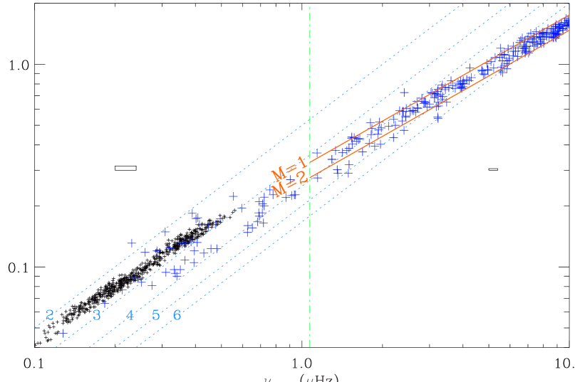
Figure 3: $\nu_{\mathrm{max}}$ – $\Delta\nu_{\mathrm{obs}}$ relation for Kepler (blue pluses) and OGLE (black symbols) AGB and RGB stars. The red solid lines indicate the isomass levels 1 and 2 $M_{\odot}$, in their domain of validity. The dotted lines indicate isolines of the number $n_{\mathrm{max}}=\nu_{\mathrm{max}}/\Delta\nu_{\mathrm{obs}}$. The vertical green dot-dashed line shows the region where the oscillation regime changes. Typical uncertainties at low and large $\nu_{\mathrm{max}}$ for Kepler data are indicated by the 1-$\sigma$ error boxes.

4 Global oscillation parameters

4.1 Measuring $\nu_{\mathrm{max}}$ at low frequency

For the location of the excess power in Kepler data, we first assume that the excitation of the modes is stochastic. It thus makes sense to measure the frequency $\nu_{\mathrm{max}}$ of the maximum oscillation signal. This hypothesis will have to be discussed a posteriori. Measuring $\nu_{\mathrm{max}}$ accurately at low frequency is challenging, because $\nu_{\mathrm{max}}$ cannot be well defined when only two or three modes are observed. Moreover, as discussed by Belkacem (2012), we lack a precise theoretical definition of $\nu_{\mathrm{max}}$. Methods usually used are operative in this low-frequency domain, but with large uncertainties (e.g. Mosser & Appourchaux 2009; Hekker et al. 2010; Kallinger et al. 2010; Huber et al. 2011). We used a very simple approach that does not rely on a fit of the oscillation excess power. A first estimate of $\nu_{\mathrm{max}}$ is derived as a function of the large separation $\Delta\nu_{\mathrm{obs}}$ derived with the EACF according to the scaling relations found at larger $\Delta\nu_{\mathrm{obs}}$ (Huber et al. 2011). It is used to define the frequency range $\mathcal{E}$ with oscillation power in excess. We then perform the weighted mean

$$\nu_{\mathrm{max}}=\int_{\mathcal{E}}\bigl{[}p(\nu)-b(\nu)\bigr{]}\;\nu\;\mathrm{d}\nu\Bigm{/}\int_{\mathcal{E}}\bigl{[}p(\nu)-b(\nu)\bigr{]}\;\mathrm{d}\nu,$$ (1)

where $p(\nu)$ is the power spectrum density observed in the frequency range $\mathcal{E}$, and $b(\nu)$ is the background component, determined with the method COR presented in Mathur et al. (2011). This method describes the background in the vicinity of the frequency range where the oscillation excess power is observed, at frequencies just below $0.4\,\nu_{\mathrm{max}}$ and just above $1.6\,\nu_{\mathrm{max}}$. Monte-Carlo simulations indicate that the precision of the measurement of $\nu_{\mathrm{max}}$ with Eq. (1) is about 15 % for a large separation of 0.1 $\mu$Hz (20 % in similar conditions when $\nu_{\mathrm{max}}$ is derived from a Gaussian fit of the smoothed spectrum). Reducing these large uncertainties with longer time series could both lower the influence of the stochastic excitation and enhance the frequency resolution of oscillation spectra.

In the following, we use $\nu_{\mathrm{max}}$ for linking with observations in the earlier stages of the RGB. However, for precise information, we prefer to use $\Delta\nu_{\mathrm{obs}}$. The $\nu_{\mathrm{max}}$ – $\Delta\nu_{\mathrm{obs}}$ relation (e.g., Hekker et al. 2009; Stello et al. 2009) is shown in Fig. 3. The measurements at low $\Delta\nu_{\mathrm{obs}}$ extend the trend at larger $\Delta\nu_{\mathrm{obs}}$, so that we have a first indication that the hypothesis of stochastic excitation is verified. We notice, however, a change of regime around 1 $\mu$Hz, associated with an apparent lack of data. The fits for Kepler stars are, below and above 1 $\mu$Hz,

$$\Delta\nu_{\mathrm{obs}} = (0.296\pm 0.004)\,\nu_{\mathrm{max}}^{0.727\pm 0.007}\ \hbox{ for }\nu_{\mathrm{max}}>1\,\mu\hbox{Hz},$$ (2)

$$\Delta\nu_{\mathrm{obs}} = (0.248\pm 0.010)\,\nu_{\mathrm{max}}^{0.783\pm 0.049}\ \hbox{ for }\nu_{\mathrm{max}}<1\,\mu\hbox{Hz},$$ (3)

with both $\Delta\nu_{\mathrm{obs}}$ and $\nu_{\mathrm{max}}$ expressed in $\mu$Hz (Fig. 3).

We note that, at low $\nu_{\mathrm{max}}$, the OGLE and Kepler relations fully agree, with a slope slightly steeper than for higher frequencies. Kepler data show a wider spread, which we interpret as due to the poorer frequency resolution and to the imprecise measurement of $\nu_{\mathrm{max}}$. The exponent remains close to three quarters, as a direct consequence of the scaling relations of the stellar mass and radius. At large $\Delta\nu_{\mathrm{obs}}$, the spread of the value around the mean fit indicated by Eq. (2) is mainly a mass effect. At low $\Delta\nu_{\mathrm{obs}}$, the spread is also due to the inaccurate measurement of $\nu_{\mathrm{max}}$. Compared to previous studies (e.g., Huber et al. 2011) we have gained more than one decade towards low frequencies in determining the validity of the $\nu_{\mathrm{max}}$ – $\Delta\nu_{\mathrm{obs}}$ relation. From this relation, we can derive the radial order $n_{\mathrm{max}}$ corresponding approximately to $\nu_{\mathrm{max}}/\Delta\nu_{\mathrm{obs}}$. As already noted by Mosser et al. (2010), this index decreases significantly when the stellar radius increases.

The change in slope noted in the $\nu_{\mathrm{max}}$ – $\Delta\nu_{\mathrm{obs}}$ relation (Fig. 3) occurs in a frequency range with an apparent lack of data. The density of stars being low, we cannot exclude that this gap is only spurious. However, we do not identify any observing bias able to produce such a gap. Then, in the absence of direct explanation, we have chosen to identify it in all figures, aiming to find an explanation.

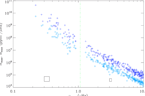
Figure 4: Maximum height $H_{\mathrm{max}}$ (blue $+$) and background power density $B_{\mathrm{max}}$ (diamonds) at $\nu_{\mathrm{max}}$, as a function of $\nu_{\mathrm{max}}$. The vertical green dot-dashed line shows the region where the oscillation regime changes. Typical uncertainties at low and large $\nu_{\mathrm{max}}$ are indicated by the 1-$\sigma$ error boxes.

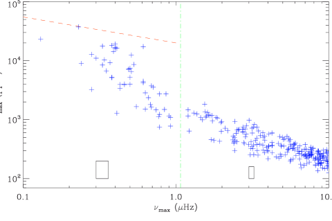
Figure 5: Same as Fig. 4 but for the maximum relative amplitude $A_{\mathrm{max}}$. The red dashed line shows the relative amplitude that causes an acceleration as strong as the surface gravity, according to the model developed in Section 8.2.

4.2 Background, maximum height

The maximum height of the power density spectrum at $\nu_{\mathrm{max}}$, the background at $\nu_{\mathrm{max}}$, and the maximum amplitude were derived from the method COR used in Mosser et al. (2012a) and Mathur et al. (2011). The variation in these parameters as a function of $\nu_{\mathrm{max}}$ is presented in Fig. 4. The scaling relations, for height and background in ppm${}^{2}\,\mu$Hz^-1 and $\nu_{\mathrm{max}}$ in $\mu$Hz, are

$$H_{\mathrm{max}} = (2.8\pm 0.2)\,10^{7}\ \nu_{\mathrm{max}}^{-2.50\pm 0.05},$$ (4)

$$B_{\mathrm{max}} = (6.2\pm 0.4)\,10^{6}\ \nu_{\mathrm{max}}^{-2.48\pm 0.04}\ \hbox{ for }\nu_{\mathrm{max}}>1\,\mu\hbox{Hz}$$ (5)

and

$$H_{\mathrm{max}} = (3.6\pm 1.1)\,10^{7}\ \nu_{\mathrm{max}}^{-4.10\pm 0.41},$$ (6)

$$B_{\mathrm{max}} = (6.3\pm 1.3)\,10^{6}\ \nu_{\mathrm{max}}^{-3.35\pm 0.30}\ \hbox{ for }\nu_{\mathrm{max}}<1\,\mu\hbox{Hz}.$$ (7)

For $\nu_{\mathrm{max}}>1\,\mu$Hz, the values of the fits are comparable to the values found by Mosser et al. (2012a) in the lower RGB and in the clump. Interestingly, the exponent of the $H_{\mathrm{max}}$ scaling relation is close to the exponent found in the RGB by Samadi et al. (2012) for the energy supply rate, varying as $(L/M)^{2.6}$, hence as $\nu_{\mathrm{max}}^{-2.6}$. This may have indirect consequences on the mode linewidth.

At very low frequency, below 0.25 $\mu$Hz, we have identified in a few cases a component that may be either a stellar signal (activity or background modulated by the surface rotation) or instrumental noise. This effect occurs at such a low frequency that it only modestly perturbs the measurement of the background of the most evolved stars, without significant consequences.

Despite the change of regime, which occurs at the same location as for the $\nu_{\mathrm{max}}$ – $\Delta\nu_{\mathrm{obs}}$ scaling relation, the continuous variation from high to low values of $\Delta\nu_{\mathrm{obs}}$ confirms the hypothesis of stochastic oscillations. The lack of stars with global parameters $\nu_{\mathrm{max}}\simeq 1\,\mu$Hz, or equivalently $\Delta\nu_{\mathrm{obs}}\simeq 0.28\,\mu$Hz, and the change of regime in all scaling relations tend to indicate a change in either the stellar structure or the upper atmospheric properties. However, in both regimes, the exponents for $H_{\mathrm{max}}(\nu_{\mathrm{max}})$ and $B_{\mathrm{max}}(\nu_{\mathrm{max}})$ are consistent. As for earlier evolutionary stages, the ratio $H_{\mathrm{max}}/B_{\mathrm{max}}$ does not vary with $\nu_{\mathrm{max}}$. This underlines that the ratio of the energy transferred from the convection in the granulation (background signal) or in the oscillation is nearly constant.

4.3 Maximum amplitude

To prepare the link with infrared ground-based data, we also investigate the mode amplitude $A_{\mathrm{max}}$ of the oscillations. This parameter can be derived from $H_{\mathrm{max}}$, with the method presented in Mosser et al. (2012a):

$$A_{\mathrm{max}} = (1.4\pm 0.1)\;10^{3}\;\nu_{\mathrm{max}}^{-0.82\pm 0.03}\ \hbox{ for }\nu_{\mathrm{max}}>1\,\mu\hbox{Hz},$$ (8)

$$A_{\mathrm{max}} = (2.0\pm 0.3)\;10^{3}\;\nu_{\mathrm{max}}^{-1.53\pm 0.21}\ \hbox{ for }\nu_{\mathrm{max}}<1\,\mu\hbox{Hz},$$ (9)

with $A_{\mathrm{max}}$ in ppm and $\nu_{\mathrm{max}}$ in $\mu$Hz. At high $\nu_{\mathrm{max}}$, we retrieve a steeper fit than previously found for the lower part of the RGB (slope of $\-0.71\pm 0.01$). At low $\nu_{\mathrm{max}}$, $A_{\mathrm{max}}$ can also be directly measured in the time series since relative photometric variations are greater than 1 mmag for red giants with $\Delta\nu\leq 0.4\,\mu$Hz (Fig. 5). Accordingly, we have estimated the mean amplitude $\sigma_{t}$ of the oscillating signal: it directly compares to $A_{\mathrm{max}}$. This extends the validity of the relation found in the RGB by Hekker et al. (2012). Extrapolation of Eq. (9) predicts $A_{\mathrm{max}}=0.75$ for modes with $\nu_{\mathrm{max}}\simeq 0.02\,\mu$Hz (periods about 580 days), hence a peak-to-valley visible magnitude change of 1.

We did not consider superimposing the OGLE data on the Kepler data in Figs. 4 and 5 since the different ways the data have been treated preclude a direct comparison. In fact, DS10 already perform a comparison, based on the amplitude measure in the I band, which agrees with the scaling relations found for RGB stars observed by CoRoT and Kepler (Mosser et al. 2010; Stello et al. 2010).

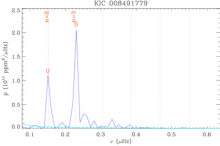
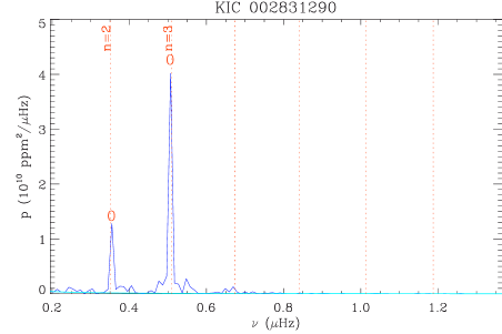
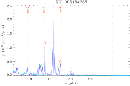
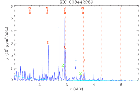
Figure 6: Typical Kepler spectra with low $\Delta\nu_{\mathrm{obs}}$. The mode identification is derived from the method presented in Section 5. Dotted lines indicate the expected location of radial modes. Modes at least eight times larger than the background (light-blue line) are labeled with their degree. The presence of multiple peaks corresponding to dipole modes indicates that they are mixed modes.

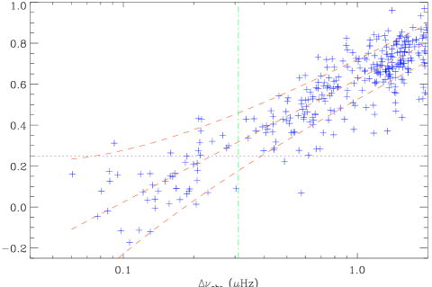
Figure 7: Relation $\varepsilon_{\mathrm{obs}}(\Delta\nu_{\mathrm{obs}})$ at low frequency. The dashed lines correspond to the fit proposed in Table 1, plus and minus the uncertainty, which mainly reflects the uncertainty on $\Delta\nu_{\mathrm{obs}}$. The horizontal dotted line shows the asymptotic value $\varepsilon_{\mathrm{as}}=1/4$.

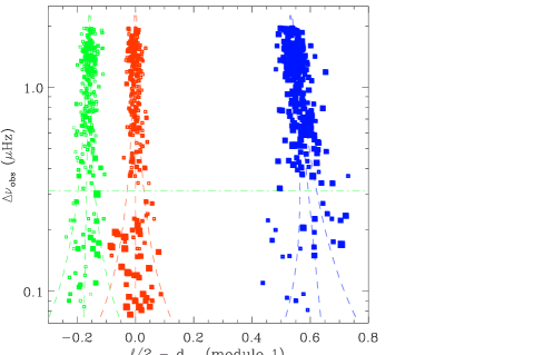
Figure 8: Variation in the terms $\ell/2-d_{0\ell}$ measuring the location of non-radial modes with respect to radial modes (Eq. 10) in abscissa, with the observed large separation in ordinate. The term $d_{00}$ in red, close to zero, indicates that the fit of $\varepsilon_{\mathrm{obs}}(\Delta\nu_{\mathrm{obs}})$ is unbiased; $0.5-d_{01}$ in blue shows a wide spread that may indicate the presence of mixed modes; $-d_{02}$ is plotted in green. The size of the symbols is proportional to the percentage of energy in a given degree. The dashed lines correspond to the fits proposed in Table 1, plus or minus the frequency resolution.

5 Individual frequencies

The mode identification for red giant oscillations observed by CoRoT and Kepler is provided in an automated way by the universal red giant oscillation pattern (Mosser et al. 2011b). It is based on the assumption that the near-homology of red giant interior structure implies the homology of the oscillation spectra, as verified by subsequent work (e.g., Corsaro et al. 2012). The method, up to now tested for $\Delta\nu\geq 0.4\,\mu$Hz and validated by comparison with other methods (Hekker et al. 2011; Verner et al. 2011; Kallinger et al. 2012; Hekker et al. 2012), has been extrapolated towards lower frequencies.

5.1 Parametrization of the spectrum

For red giants, it is useful to express the radial and low-degree mode frequencies from the analytical expression (Mosser et al. 2011b)

$$\nu_{n,\ell}=\left(n+\varepsilon_{\mathrm{obs}}+{\alpha_{\mathrm{obs}}\over 2}\;[n-n_{\mathrm{max}}]^{2}+{\ell\over 2}-d_{0\ell}\right)\Delta\nu_{\mathrm{obs}}.$$ (10)

The first three terms ($n$, $\varepsilon_{\mathrm{obs}}$, and the second-order correction in $\alpha_{\mathrm{obs}}$) provide the expected mean location of the radial modes, independent of small modulations that are due to inner-structure discontinuities (e.g., Miglio et al. 2010). Compared to the radial modes, the relative positions of dipole and quadrupole modes differ by the terms $\ell/2-d_{0\ell}$.

The dimensionless term $n_{\mathrm{max}}$, defined as $\nu_{\mathrm{max}}/\Delta\nu_{\mathrm{obs}}-\varepsilon_{\mathrm{obs}}$, is introduced in Eq. (10) to allow for the fact that the large separation $\Delta\nu_{\mathrm{obs}}$ is measured in a frequency range centered on $\nu_{\mathrm{max}}$. The curvature term $\alpha_{\mathrm{obs}}$ expresses the second-order contribution of the asymptotic expansion. It varies as $0.076/n_{\mathrm{max}}$ for less-evolved red giants (Mosser et al. 2013); this implies a significant gradient for low $n_{\mathrm{max}}$, as high as 4 %, of the frequency separation between consecutive radial modes. We note that such a gradient is clearly observed in the spectra of M giants reported by Tabur et al. (2010), which does not necessarily correspond to the gradient expressed by $\alpha_{\mathrm{obs}}$ since significant departure from the asymptotic expansion is expected at very low radial order.

We chose to express the dependence of the parameters $\varepsilon_{\mathrm{obs}}$, $\alpha_{\mathrm{obs}}$, and $d_{0\ell}$ with a term $\log_{10}\Delta\nu_{\mathrm{obs}}$, as in Mosser et al. (2011b). Owing to the possibility that dipole modes behave as mixed modes, we did not fix their position during the analysis. We also considered that the influence of rotation is negligible. Extrapolation from Mosser et al. (2012b) indicates that the transfer of angular momentum between the envelope and the core is efficient enough for ensuring very small splittings of the dipole modes either on the upper RGB or on the AGB.

Table 1: Fits of the low-degree ridges

	$\ell$	fit $A_{\ell}+B_{\ell}\log\Delta\nu_{\mathrm{obs}}$
		$A_{\ell}$	$B_{\ell}$
$\varepsilon_{\mathrm{obs}}$	0	$0.623\pm 0.006$	$0.599\pm 0.015$
$d_{01}$	1	$-0.057\pm 0.003$	$0.070\pm 0.007$
$d_{02}$	2	$0.162\pm 0.002$	$-0.013\pm 0.004$
$\alpha_{\mathrm{obs}}$	all	$0.076\ \Delta\nu_{\mathrm{obs}}/\nu_{\mathrm{max}}$

These fits are valid for observed large separations $\Delta\nu_{\mathrm{obs}}$ in the range [0.1 – 2 $\mu$Hz].

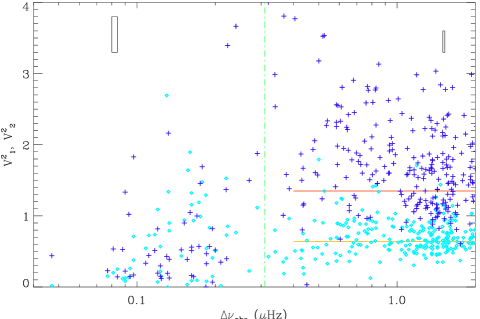
Figure 9: Dipole (dark blue $+$) and quadrupole mode (light blue diamonds) visibilities, as a function of the observed large separation. The horizontal lines indicate the respective fits found by Mosser et al. (2012a) at larger $\Delta\nu_{\mathrm{obs}}$. The vertical green dot-dashed line shows the region where the oscillation regime changes.

5.2 Mode identification

As already done by Mosser et al. (2011b) for CoRoT RGB and red clump stars, the use of Eq. (10) provides a refined measurement of $\Delta\nu_{\mathrm{obs}}$ and allows complete identification of all low-frequency spectra. The extrapolation towards very low frequencies was made possible by the continuous distribution of giants at all evolutionary stages. A few examples are shown in Fig. 6.

The efficiency of the method is proven by the capability of fitting all major peaks of the spectra, defined by a height-to-background ratio over eight. The parameters of the fit were iteratively improved. This provides a small correction of the $\varepsilon_{\mathrm{obs}}(\Delta\nu_{\mathrm{obs}})$ relation introduced by Mosser et al. (2011b), as plotted in Fig. 7.

From the radial modes actually identified with Eq. (10), we derived new values for the large separation and for the offset and provided a new fit of the radial-mode oscillation pattern (Table 1). An échelle diagram shows the efficiency of the method (Fig. 8). All peaks with a height-to-background ratio greater than eight are plotted. Glitches are present, with a greater relative weight than at larger $\Delta\nu_{\mathrm{obs}}$, on the order of $\pm 0.05\Delta\nu_{\mathrm{obs}}$. There is an indication that, even at low $\Delta\nu_{\mathrm{obs}}$, dipole modes appear to be mixed since more than one peak per radial order is often seen. However, their period spacing cannot be estimated since the frequency resolution is not sufficient to resolve consecutive mixed orders. The size of the symbols in Fig. 8 is proportional to the total energy integrated for each degree. From these measurements, we find that dipole modes dominate at large $\Delta\nu_{\mathrm{obs}}$, whereas radial modes dominate at low $\Delta\nu_{\mathrm{obs}}$. The change in regime occurs again in the same region.

Mosser et al. (2013) have shown that Eq. (10) is a form equivalent to the asymptotic expansion, based on the observed value of the radial frequency separation, which is different from the asymptotic value. Here, we use it at very low radial order to provide the mode identification. An operative fit does not imply that the oscillation pattern follows the asymptotic expansion. In fact, a significant departure to asymptotics is seen in the function $\varepsilon_{\mathrm{obs}}$, valid for $\Delta\nu_{\mathrm{obs}}$ down to 0.1 $\mu$Hz. According to the link between observed and asymptotic parameters, we should have $\varepsilon_{\mathrm{obs}}\geq 1/4$ (Mosser et al. 2013). This is clearly not the case since negative values of $\varepsilon_{\mathrm{obs}}$ are found at very low $\Delta\nu_{\mathrm{obs}}$. In fact, the deviation from the asymptotic pattern at radial orders as low as 2 is expected.

5.3 Mode visibilities

The degrees of the observed modes could not, so far, be determined from ground-based microlensing surveys. Observationally, most often only radial modes were searched for, even if the presence of non-radial modes was suspected. In luminous red giants, all non-radial modes suffer high radiative losses in stellar cores. However, for some (one for each $\ell$ per radial mode), the efficient trapping in the envelope ensures that these losses are negligible in the overall energy budget (Dupret et al. 2009; Dziembowski 2012). The expected oscillation spectrum then again becomes as simple as in unevolved non-rotating stars.

The location of radial modes and the resulting full identification of the oscillation pattern in the Kepler data allows us to measure the visibilities of the modes, depending on the degree, with the method proposed by Mosser et al. (2012a). Visibilities measure the mean height of the modes associated to each degree, calibrated to the mean height of radial modes. We did not search for $\ell=3$ modes since insufficient frequency resolution hampers their detection at low frequency. Our results are given in Fig. 9. We identify three regimes.

• For large separations over 0.6 $\mu$Hz, the measured visibilities $V^{2}_{1}$ and $V^{2}_{2}$ have a mean value of about 1.5 and 0.6, respectively, in agreement with the measurements done at high $\nu_{\mathrm{max}}$ (Mosser et al. 2012a). Their distributions show a wide spread, which we identify as the result of the small numbers of significantly excited modes.

• For large separations in the range [0.2 – 0.6 $\mu$Hz], in the domain where we observed the change in regime of previous scaling relations, we note a huge spread of the visibility distributions. Again, we interpret this as a result of the stochastic excitation, amplified by the fact that only a limited number of modes are visible. Most of the oscillation energy is often concentrated in one major peak, close to $\nu_{\mathrm{max}}$, which can have any degree since radial and non-radial are simultaneously visible. The degree ${\ell_{\mathrm{max}}}$ of this peak is associated to a dominant visibility $V^{2}_{\ell_{\mathrm{max}}}$.

• At lower large separations, we note a rapid decrease in the non-radial mode visibilities, both for dipole and quadrupole modes. For large separations below 0.2 $\mu$Hz, the damping is severe, so that only radial modes subsist with non-negligible amplitudes.

5.4 Large frequency separations in OGLE data

Large separations of oscillation spectra observed by the OGLE survey were obtained according to the parametrization expressed by Eq. (10). For $\Delta\nu_{\mathrm{obs}}$ larger than 0.2 $\mu$Hz, this new treatment did not modify the first guess of the large separations obtained in Section 3.2. At very low $\Delta\nu_{\mathrm{obs}}$, we noted a small change between the large separations derived from the frequency difference between consecutive radial orders or from the fit of Eq. (10). This change increases when the large separation decreases, and reaches a value of about 15 % at the lowest $\Delta\nu_{\mathrm{obs}}$.

This indicates that the almost constant large separation supposed in Eq. (10) is only an approximation. At very low radial orders ($n\leq 3$), a gradient is observed that is larger than the gradient inferred from the asymptotic expansion. This gradient cannot be seen in Kepler data because of the poorer frequency resolution. The full characterization of the parametrization of the spectrum at very low radial orders will require a dedicated study, which is beyond the scope of this paper.

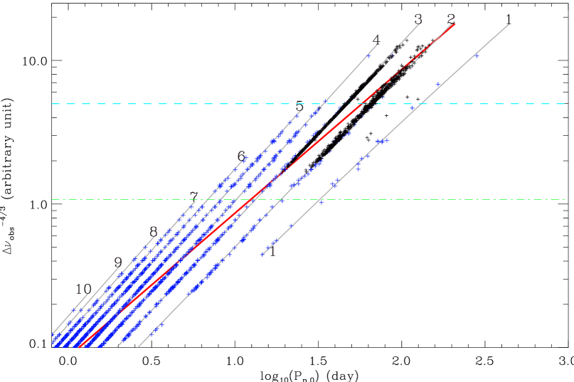
Figure 10: PL relations of radial modes of AGB and RGB stars observed with Kepler (blue pluses) and OGLE (black symbols). The proxy of the luminosity is derived from the estimate $\Delta\nu_{\mathrm{obs}}^{-4/3}$. Each sequence, corresponding to a fixed radial order, is fitted with the model provided by Eq. (10) (gray solid lines). The thick red line, provided by $\nu_{\mathrm{max}}\simeq 1/P$, indicates the the location of ratio $n_{\mathrm{max}}=\nu_{\mathrm{max}}/\Delta\nu-\varepsilon_{\mathrm{obs}}$. The blue dashed line corresponds to the tip of the RGB. The horizontal green dot-dashed lines shows the region where the oscillation regime changes.

6 Identification of the period-luminosity sequences

Ground-based infrared survey results are most often presented with PL sequences. In this section, we first aim to verify that the solar-like oscillation pattern correspond to the PL sequences and to provide an unambiguous identification of the observed sequences. Second, we explore the consequence of this link.

6.1 Seismic proxy of the luminosity

Assessing PL relations requires determining the periods and the luminosity. For field objects observed with Kepler, determining the luminosity can be done indirectly. A proxy of the luminosity can be obtained from the black body relation. This requires the use of effective temperature, provided by the Kepler Input Catalog (Brown et al. 2011). From this catalog, we find that ${T_{\mathrm{eff}}}$ varies as $\Delta\nu_{\mathrm{obs}}^{0.068\pm 0.011}$ for our cohort of red giants.

From the black body relation and the $\nu_{\mathrm{max}}$ scaling relation (Belkacem et al. 2011), the luminosity scales as $L\propto M\;{T_{\mathrm{eff}}}^{7/2}\;\nu_{\mathrm{max}}^{-1}$. Since $\nu_{\mathrm{max}}$ suffers from large uncertainties, we prefer to use the proxy

$$L\propto M^{2/3}\;{T_{\mathrm{eff}}}^{4}\;\nu_{0}^{-4/3},$$ (11)

with the dynamical frequency $\nu_{0}$ for scaling as $\sqrt{M/R^{3}}$. We prefer not to use the asymptotic large separation $\Delta\nu_{\mathrm{as}}$, since an asymptotic value of the large separation is not useful at such low orders.

Equation (11) is based on the assumption that $\nu_{\mathrm{max}}\propto\nu_{0}^{3/4}$. At this stage, we are not able to relate $\nu_{0}$ and $\Delta\nu_{\mathrm{obs}}$, but first assume that they are comparable. We have plotted $\Delta\nu_{\mathrm{obs}}^{-4/3}$ as a function of the periods of the observed radial modes (Fig. 10). Doing so is in practice equivalent to supposing that all stars have the same mass. This is justified because the oscillation pattern hardly depends on the stellar mass (Xiong & Deng 2007). For our set of data, we may assume that the mean stellar mass is of about 1.3 $M_{\odot}$, according to the mean value derived for the cohort of red giants observed at higher $\nu_{\mathrm{max}}$ (Kallinger et al. 2010; Mosser et al. 2012c).

6.2 Identification of the sequences

The identification of the PL relations (as in Fig. 1 of S07) can be obtained at this stage, following the stellar evolution from the high-$\Delta\nu_{\mathrm{obs}}$ region, where pulsations are precisely depicted, down to lower values where OSARG oscillations are seen. The construction of a PL diagram with $\Delta\nu_{\mathrm{obs}}^{-4/3}$ as a proxy of the luminosity provides a unique solution for identifying the sequences observed in PL relations (Fig. 10).

We note that, apart from a few points that represent fewer than 0.5 % of the measured periods, all periods fit the theoretical ridges. The OGLE sequences $b_{2}$ and $b_{3}$ closely correspond to the sequences with radial orders 2 and 3, respectively. This proves that the identification proposed by DS10 is correct. Oscillations in OSARG, and more generally in semi-regular variables (SRV), are solar-like oscillations. A summary of the identification of the sequences observed in SRV is given in Table 2.

Table 2: Equivalence between solar-like oscillations (labeled with the radial order $n$) and PL sequences

$n$	sequences	pulsations
1	$b_{1}$	fundamental of semi-regular variables (SRV)
2	$b_{2}$	1st overtone of SRV
3	$b_{3}$	2nd overtone of SRV
4	…	…
$n_{\mathrm{max}}\simeq 8$		clump stars
$n_{\mathrm{max}}\simeq 15$		lower RGB
$n_{\mathrm{max}}\simeq 22$		Sun

6.3 Period-luminosity relation in the K band

Usually, PL relations are expressed either with the brightness in the K bandwidth or with a Wesenheit index for avoiding reddening issues (Madore 1982). Here, we intend to calibrate PL relations with the K magnitude. It depends on the effective temperature, with an exponent $k=\mathrm{dlog}\,L_{\mathrm{K}}/\mathrm{dlog}\,T$, derived from the black body radiance, in the range [1.9, 2.1] for the effective temperatures in the sample of stars (Table 3). We consider $\langle k\rangle\simeq 2.04$ as a reliable mean value in the relation between the brightness $L_{\mathrm{K}}$ in the K band and the large separation $\nu_{0}$. At fixed mass, we then have from Eq. (11)

$$\mathrm{dlog}\,L_{\mathrm{K}}=-{4\over 3}\ \mathrm{dlog}\,\nu_{0}+\langle k\rangle\ \mathrm{dlog}\,{T_{\mathrm{eff}}}.$$ (12)

Here, we need to introduce a relation between $\Delta\nu_{\mathrm{obs}}$ and $\nu_{0}$, which we empirically choose to write as a power law:

$$\mathrm{dlog}\,\nu_{0}=\gamma\ \mathrm{dlog}\,\Delta\nu_{\mathrm{obs}}.$$ (13)

The exponent $\gamma$, presumably close to 1, remains unknown at this stage. From the KIC temperatures (Brown et al. 2011), we derive the mean relation between ${T_{\mathrm{eff}}}$ and $\Delta\nu_{\mathrm{obs}}$:

$$\mathrm{dlog}\,{T_{\mathrm{eff}}}=t\ \mathrm{dlog}\,\Delta\nu_{\mathrm{obs}},$$ (14)

with $t$ about 0.068. Finally, we can derive the evolution of the magnitude in the K band with the observed large separation:

$$\mathrm{d}K=2.5\left({4\over 3}\ \gamma-\langle k\rangle t\right)\mathrm{dlog}\,\Delta\nu_{\mathrm{obs}}.$$ (15)

This relation is established following the variation in the observed large frequency separation $\Delta\nu_{\mathrm{obs}}$. It is therefore representative of stellar evolution and does not correspond to any PL sequence. In a next step, we have to retrieve the PL relation for each observed sequence.

Table 3: Exponent $\langle k\rangle$ in the K band

${T_{\mathrm{eff}}}$	$k(\lambda)$			$\langle k\rangle$
(K)	2.0	2.2	2.4
3800	2.23	2.10	1.99	2.10
4000	2.16	2.03	1.93	2.04
4200	2.09	1.97	1.88	1.98
4700 (clump)	1.95	1.85	1.77	1.86

6.4 Period-luminosity sequences in the K band

The PL relations are a given set of different observed sequences, each supposedly corresponding to a fixed radial order $n$. We note $\Delta K_{n}$ the variation in the magnitude along the sequence corresponding to radial order $n$. We have to consider the difference between the slopes of the PL sequences (at fixed radial order) and the slope following stellar evolution (with the radial orders $n$ of the observable modes evolving as $n_{\mathrm{max}}$). With the proxy of the luminosity plotted in Fig. 10 and with ${\nu_{\mathrm{max}}}^{-1}$ being considered as representative of the mean period observed, we derive

$$\mathrm{dlog}\,P\simeq-\mathrm{dlog}\,\nu_{\mathrm{max}}=-p_{n}\ {\mathrm{dlog}\,{\nu_{\mathrm{max}}}\over\mathrm{dlog}\,\Delta\nu_{\mathrm{obs}}}\ \mathrm{dlog}\,P_{n},$$

where the derivatives $p_{n}$ of the relations $P_{n}=1/\nu_{n,0}$, defined by

$$\mathrm{dlog}\,\Delta\nu_{\mathrm{obs}}=p_{n}\ \mathrm{dlog}\,P_{n},$$ (16)

are estimated from Eq. (10). The relation between stellar evolution and individual sequences is thus expressed by

$${\mathrm{d}K_{n}\over\mathrm{dlog}\,P_{n}}=-p_{n}\ {\mathrm{dlog}\,\nu_{\mathrm{max}}\over\mathrm{dlog}\,\Delta\nu_{\mathrm{obs}}}\left.{\mathrm{d}K\over\mathrm{dlog}\,P}\right|_{n_{\mathrm{max}}}.$$ (17)

From Eqs (15)-(17), we finally obtain the variation in the K magnitude with period on a given sequence:

$$\Delta K_{n}\propto-2.5\ p_{n}^{2}\left({4\over 3}\ \gamma-\langle k\rangle t\right){\mathrm{dlog}\,\nu_{\mathrm{max}}\over\mathrm{dlog}\,\Delta\nu_{\mathrm{obs}}}\ \Delta\!\log P_{n}.$$ (18)

With this result, it is now possible to interpret the slopes $\Delta K_{n}/\Delta\!\log P_{n}$ reported by S07. In Table 4, we derive a mean value $\gamma$ for the sequences $n=1$ to 3 observed by S07 in the Magellanic Clouds.

Table 4: Sequences in the period-luminosity diagram

radial order $n$	1	2	3
slope $p_{n}$	$-0.847$	$-0.902$	$-0.932$
LMC sequence (S07)	b1	b2	b3
$\mathrm{d}K_{\mathrm{S}}/\mathrm{dlog}\,P_{n}$	$-3.34$	$-3.58$	$-3.72$
$\gamma_{n}$	1.16	1.10	1.07
SMC sequence (S07)	b1	b2	b3
$\mathrm{d}K_{\mathrm{S}}/\mathrm{dlog}\,P_{n}$	$-3.56$	$-3.88$	$-4.40$
$\gamma_{n}$	1.22	1.18	1.25

Table 5: Absolute seismic calibration

$K$	$\nu_{\mathrm{max}}$	$\Delta\nu_{\mathrm{obs}}$	$\nu_{0}$	${T_{\mathrm{eff}}}$	$\gamma$	$k$	$R_{0}$
	($\mu$Hz)	($\mu$Hz)	($\mu$Hz)	(K)			($R_{\odot}$)
$-$8.55	0.05	0.024	0.016	3355	1.21	2.28	929
$-$8.06	0.07	0.033	0.023	3422	1.21	2.25	666
$-$7.58	0.11	0.044	0.033	3489	1.21	2.22	477
$-$7.10	0.15	0.059	0.047	3557	1.20	2.20	342
Tip of the RGB
$-$6.63	0.22	0.080	0.067	3626	1.19	2.17	246
$-$6.16	0.32	0.108	0.095	3695	1.17	2.14	177
$-$5.70	0.46	0.145	0.134	3763	1.14	2.12	128
$-$5.26	0.66	0.195	0.187	3833	1.11	2.09	94.9
$-$4.83	0.94	0.262	0.260	3905	1.08	2.07	71.4
$-$4.42	1.36	0.353	0.356	3979	1.05	2.05	55.2
$-$4.02	1.98	0.475	0.486	4057	1.03	2.02	43.7
$-$3.63	2.91	0.640	0.659	4138	1.02	2.00	35.2
$-$3.24	4.30	0.861	0.890	4223	1.01	1.97	28.8
$-$2.85	6.38	1.16	1.20	4309	1.01	1.95	23.7
$-$2.47	9.48	1.56	1.62	4398	1.00	1.93	19.6
$-$2.09	14.1	2.10	2.18	4489	1.00	1.91	16.2
$-$1.70	21.0	2.83	2.94	4583	1.00	1.88	13.5
$-$1.32	31.3	3.80	3.95	4678	1.00	1.86	11.2

Variation with the K magnitude of the mean global seismic parameters and of the parameters used for the relation between the large separation $\Delta\nu_{\mathrm{obs}}$ and $\nu_{0}$. $R_{0}$ is the stellar radius derived from the scaling relation based on $\nu_{0}$.

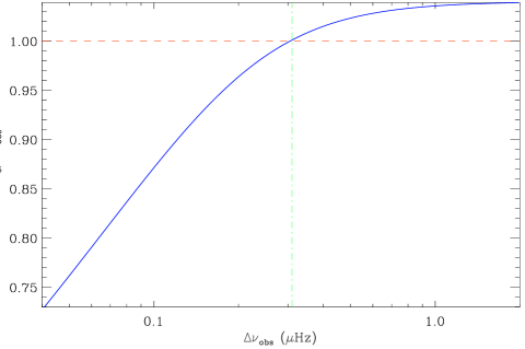
Figure 11: Ratio $\nu_{0}/\Delta\nu_{\mathrm{obs}}$ as a function of $\Delta\nu_{\mathrm{obs}}$, scaled according to the calibration derived from ground-based PL relations. The dashed line indicates the 1:1 relation. The vertical green dot-dashed lines shows the region where the oscillation regime changes.

7 Calibration of the period-luminosity relation

From the identification of the sequences, we can derive the factor $\gamma=\mathrm{dlog}\,\nu_{0}/\mathrm{dlog}\,\Delta\nu_{\mathrm{obs}}$. Firstly, this opens the possibility of measuring the mean stellar density from seismic analysis in non-asymptotic conditions, under the hypothesis that the scaling relation between $\nu_{\mathrm{max}}$ and the acoustic cutoff frequency is valid. Secondly, we can integrate Eq. (15).

7.1 Calibration of the mean stellar density

We have derived estimates $\gamma_{n}$ of $\gamma$ for each sequence, according to Eq. (18). Results are shown in Table 4. We note a relative agreement better than 3 % between the coefficients $\gamma_{n}$ for the LMC and SMC separately, even if we do not interpret the 7 % differences of the slopes reported in the SMC and LMC by S07.

Since the dependence of $\gamma_{n}$ in $n$ is less than the uncertainties, we consider that the mean value of the $\gamma_{n}$ is representative of the scaling relation relating $\nu_{0}$ to $\Delta\nu_{\mathrm{obs}}$ at very low frequency:

$$\gamma\simeq 1.17\pm 0.08.$$ (19)

That the observed coefficient $\gamma$ is close to unity indicates that $\Delta\nu_{\mathrm{obs}}$ provides a good proxy of a $\nu_{0}$. However, non-negligible divergence between these large separations may appear when integrating Eq. (13) with the result of Eq. (19).

We have built an empirical relation between the observed spacing $\Delta\nu_{\mathrm{obs}}$ and the dynamical frequency $\nu_{0}$, which assumes a smoothly varying $\gamma$ coefficient between the different regimes depending on stellar evolution. For the most-evolved stages, at very low $\Delta\nu_{\mathrm{obs}}$, the value of $\gamma$ is given by Eq. (19); for less-evolved stages, at larger $\Delta\nu_{\mathrm{obs}}$, it corresponds to $\nu_{0}\simeq\Delta\nu_{\mathrm{as}}\simeq 1.038\,\Delta\nu_{\mathrm{obs}}$ (Mosser et al. 2013). The resulting model is shown in Fig. 11. We have imposed the change of regime (i.e. a smoothed change of $\gamma$) at $\Delta\nu_{\mathrm{obs}}=0.3\,\mu$Hz, in agreement with the observation. This toy model is only a possible solution, so it awaits a theoretical justification. We use it in Section 7.3 to investigate the consequences of the scaling provided by Eq. (19).

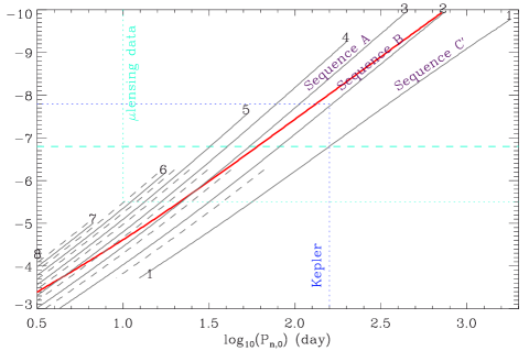
Figure 12: Synthetic PL relations as proposed in Fig. 10, but calibrated in K magnitude. Dipole modes (dashed lines) are included for observed large separations down to $0.1\,\mu$Hz. PL relations have been extrapolated towards bright magnitudes and long periods. The dotted lines delimit the region of Kepler observations with $\nu_{\mathrm{max}}\geq 0.15\,\mu$Hz, and of OGLE observations with $\nu_{\mathrm{max}}\leq 0.6\,\mu$Hz. Sequences A, B, and C’ identified at high luminosity by S07 are indicated.

7.2 New calibration

With the determination of $\gamma$, it becomes possible to integrate Eq. (15), in order to relate the K magnitude to the observed large separation. We have based the calibration in $K$ on the sequences measured in the Large Magellanic Cloud by Soszyński et al. (2007), taking the distance modulus $\mu_{\mathrm{LMC}}=18.49$ into account (Pietrzyński et al. 2013). The variations in the parameter $\gamma$ allow us to integrate the evolution from the range where OGLE measurements are made, encompassing the tip of the RGB (K magnitude of $-6.8$ in the solar neighborhood, according to Tabur et al. 2009), to the red clump ($K$ magnitude about $-1.57$, according to van Helshoecht & Groenewegen 2007).

Table 5 shows different variables used for the calibration: frequency $\nu_{\mathrm{max}}$, effective temperature, and parameters used for integrating Eq. (15). We estimate that the uncertainty of the calibration in $K$ is about 0.25. The PL sequences plotted in Fig. 12 take this calibration into account. At low luminosity, sequences show a smooth curvature, which is not depicted by the linear slope (in log scale) reported by previous work since it occurs at periods that are too short. In the OSARG domain, the sequences are drawn by the decrease in the radial frequencies with stellar evolution. When an RGB or AGB star evolves, its large separation decreases and the observable radial orders decrease, too, from a mean value $n_{\mathrm{max}}\simeq 8$ at the clump down to $n_{\mathrm{max}}\simeq 3$ at the tip of the RGB, and down to $n=2$ or 1 for the most evolved semi-regular variables. We note that the models of T13 do not reproduce this scheme, since their theoretical sequences are not parallel to the observed sequences.

At this stage, this seismic calibration is the same for RGB and AGB stars, unlike classical PL relations (Kiss & Bedding 2003). Further observations of the red giants at known distance will help improve the calibration, and more modeling will help for understanding it.

7.3 Scaling relations

Previous asteroseismic work has shown that estimates of the stellar mass and radius can be derived from seismic scaling relations (e.g., Kallinger et al. 2010; Mosser et al. 2010). Continuing efforts are being made for improving the accuracy of these relations: calibration with grid-based modeling (White et al. 2011), correction for evolution (Miglio et al. 2012), correction of bias, and calibration resulting from the comparison of modeled stars and second-order asymptotic information (Mosser et al. 2013).

In this work, we propose a similar scaling relation, but derived from the determination of $\nu_{0}$ provided by Kepler and ground-based observations. Results for the variation in the mean stellar radius with evolution are shown in Table 5. The ratio $\nu_{0}/\Delta\nu_{\mathrm{obs}}$, which is supposed to be close to 1.04 in the red giant regime corresponding to the lower RGB (Mosser et al. 2013), decreases significantly when the frequency decreases. As a consequence, scaling relations using $\Delta\nu_{\mathrm{obs}}$ are only approximate. Further modeling, similar to White et al. (2011), will help for investigating this in more detail and for tightening the link between $\Delta\nu_{\mathrm{obs}}$ and $\nu_{0}$.

8 Discussion

In this section, we intend to show how the stochastic nature of solar-like oscillations helps for understanding some characteristics of PL features. Firstly, the amplitudes of the oscillations can explain the emergence of significant mass loss. More speculative results concern the determination of the stellar evolutionary status and the nature of the change of regime detected below the tip of the RGB. Last but not least, we investigate how this work and all the information compiled by PL analysis can interact to provide refined distance scales.

8.1 Stochastic oscillations versus Mira variability

With statistical arguments, Christensen-Dalsgaard et al. (2001) have suggested that oscillations in semi-regular variables are stochastically excited. A similar conclusion was reached by Bedding et al. (2005) for the star $L_{2}$ Puppis. Further work by DS10 and T13 has shown that PL relations are drawn by stochastically excited oscillations. Here, the identification of PL relations with solar-like oscillations confirms this. The measurements of complex visibility function, with clear contributions of non-radial modes, reinforce this interpretation.

Semi-regular variables are red giants on the RGB or AGB. Semi-regularity is due to the small number of stochastically excited oscillation modes that are observed. Their complex beating and evolution with time are enough for explaining the changes. The scaling relation of $A_{\mathrm{max}}$ (Eq. 9), translated in magnitude variation, fits with microlensing results (e.g., Derekas et al. 2006; Nicholls et al. 2010). We note that variations of about one magnitude for oscillation periods about 500 days are compatible with the extrapolation of the scaling relation of $A_{\mathrm{max}}$. However, much larger amplitudes, as reported by Fraser et al. (2005), cannot be explained.

As expected, the Mira variability, with amplitudes of a few magnitudes, cannot be interpreted in terms of solar-like oscillation pressure modes. As stars in the instability strip, the Mira stars seem to obey a specific oscillation pattern, which does not correspond to solar-like oscillations. At this stage, it is not possible to provide an unambiguous identification of the radial order and degree of sequences C and D identified by ground-based measurements (S07).

8.2 Perturbation to hydrostatic equilibrium and mass loss

The measurement of the maximum amplitude $A_{\mathrm{max}}$ has shown that high values are attained when stars climb the AGB. The link between the maximum amplitude and the relative displacement $\delta R/R$ helps us understand the result of Glass et al. (2009), who state that massive mass loss is seen for main periods longer than 60 days (corresponding to $\nu_{\mathrm{max}}\simeq 0.2\,\mu$Hz).

The surface gravity can be expressed as a function of the large separation as

$$g={\mathcal{G}M\over R^{2}}\simeq(\alpha\Delta\nu_{\mathrm{obs}})^{2}\ R,$$ (20)

with $\alpha\simeq 3.6$ according to a mean estimate derived from our work. The acceleration of the oscillation associated to a displacement $\delta R$ is related to $\nu_{\mathrm{max}}$ by

$$a=(2\pi\nu_{\mathrm{max}})^{2}\ \delta R.$$ (21)

Equality between $a$ and $g$ is reached when

$${\delta R\over R}\simeq{0.36\over n_{\mathrm{max}}^{2}}.$$ (22)

In the K band, the relative brightness fluctuations depend on the relative Lagrangian radius and temperature variations

$${\delta L_{\mathrm{K}}\over L_{\mathrm{K}}}=2\ {\delta R\over R}+\langle k\rangle\ {\delta{T_{\mathrm{eff}}}\over{T_{\mathrm{eff}}}}.$$ (23)

As seen in Section 4.3, the maximum value of $\delta L_{\mathrm{K}}/L_{\mathrm{K}}$ corresponds to the maximum amplitude $A_{\mathrm{max}}$ derived from the power spectrum. In adiabatic conditions, the relative brightness variation reduces to the temperature contribution. This results from the fact that the relative radius and effective temperature Lagrangian changes are related by

$${\delta R\over H_{\mathrm{p}}}=-{\Gamma_{1}\over\Gamma_{1}-1}\ {\delta{T_{\mathrm{eff}}}\over{T_{\mathrm{eff}}}},$$ (24)

where $\Gamma_{1}$ is the local adiabatic exponent, and $H_{\mathrm{p}}$ the pressure scale height (e.g., Mosser 1995). In a spherically symmetric unperturbed star, the pressure scale height in the photosphere is much less than the stellar radius, which explains that $A_{\mathrm{max}}\simeq\langle k\rangle\,|\delta{T_{\mathrm{eff}}}/{T_{\mathrm{eff}}}|$. However, in conditions where ${T_{\mathrm{eff}}}$ presents important relative variation, hydrostatic equilibrium may not be met in the upper envelope, so that Eq. (24) may be not valid.

We therefore investigated the case where the term ${\delta R/R}$ significantly contributes to $A_{\mathrm{max}}$. The relation $A_{\mathrm{max}}=2\,|{\delta R/R}|$, superimposed on the observed amplitudes (Fig. 5), then helps to quantify the results of Glass et al. (2009): the observed maximum amplitude corresponding to $a=g$ occurs for $\nu_{\mathrm{max}}\simeq 0.2\,\mu$Hz. The quantitative coincidence is puzzling and shows that the possible disruption of the external layers of evolved red giants has to be investigated. Qualitatively, efficient mass loss certainly occurs when the oscillation amplitude in the external layers is large enough for imposing an oscillation acceleration comparable to the surface gravity. As a result, the uppermost regions are no longer firmly linked to the envelope and can be easily ejected.

8.3 AGB versus RGB

In S07, sequences labeled with $a$ (respectively $b$) correspond to stars on the AGB (respectively on the RGB). We tried to test different ways able to similarly disentangle AGB from RGB stars with Kepler asteroseismic data.

Bedding et al. (2011) and Mosser et al. (2011a) have shown that mixed modes provide a discriminating test between RGB and clump stars. Unfortunately, the impossibility of measuring mixed-mode spacings at low $\Delta\nu_{\mathrm{obs}}$ precludes a similar use for identifying the evolutionary status. Independent of the mixed mode pattern, the exact location of the radial modes also helps distinguish RGB from red clump stars (Kallinger et al. 2012). At the moment, we lack information on the fine structure of the oscillation spectra in the upper RGB to perform a similar investigation. Because AGB stars have higher ${T_{\mathrm{eff}}}$ than RGB stars, we also tried to compare the oscillation patterns depending on ${T_{\mathrm{eff}}}$, but failed to identify firm signatures.

At this stage, we are left with a degeneracy between the oscillation spectra of AGB and RGB stars observed with Kepler. The comparison with ground-based observations will help remove it.

8.4 Regime change

We have seen many changes occurring around $\nu_{\mathrm{max}}\simeq 1\,\mu$Hz. At this stage, we have no definitive explanation. We may imagine that non-linear effects become strong enough when $A_{\mathrm{max}}$ is larger than $10^{-3}$. Alternatively, if a majority of AGB stars are seen at this stage, this could be the signature of the third dredge-up. Such a signature could explain the lack of stars, since the input of heavy elements in the envelope may have boosted the evolution along the AGB. Again, the wealth of information obtained with ground-based surveys will help ascertain this.

8.5 Distance scale and microlensing surveys

The parametrization of the solar-like oscillation spectrum at low frequency and the measurement of the mode visibility developed for the Kepler giants, corrected for the gradient seen at very low $\Delta\nu_{\mathrm{obs}}$, can be used to analyze ground-based data from a microlensing survey. Identifying pulsations in evolved red giants with solar-like oscillations will help refine our understanding of the distance measurements provided by the PL relations (e.g., Feast 2004), since the analysis can now stand on a firm basis.

Periods can be precisely measured and interpreted with more accurate PL relations. Asteroseismology is in fact unable to provide the zero point of the PL relations, but can provide accurate slopes that vary with $\nu_{\mathrm{max}}$ (Fig. 12). With the explanation proposed by our Kepler measurements, the difference in PL slopes between the LMC and the SMC is surprising (Table 4): we do not expect the influence to the metallicity to be important. Observationally, PL relations do not depend on metallicity, as derived from the observation in a large number of infrared wavelengths (Schultheis et al. 2009). This result is fully compatible with solar-like oscillations. Theoretically, simulations of non-adiabatic oscillations in red giants have shown that the oscillation hardly depends on mass and metallicity (Xiong & Deng 2007). In fact, metallicity acts on $\nu_{\mathrm{max}}$, hence on the luminosity, essentially through the influence of the Mach number (e.g., Samadi et al. 2010; Belkacem et al. 2011). However, recent work shows that the $\nu_{\mathrm{max}}$ – $\nu_{\mathrm{c}}$ relation hardly depends on the Mach number for red giants (Belkacem et al. 2013), which lowers the influence of metallicity.

Analyzing the microlensing data again, taking the analytical description of the oscillation pattern depicted by Eq. (10) into account, will be fruitful, since the refined seismic analysis will benefit from microlensing information. As a consequence, population studies and distance measurements can be boosted with the new tool and paradigm proposed by our work.

9 Conclusion

We have confirmed that PL relations in evolved red giants are due to solar-like oscillations. This was done with an analytical description of the oscillation spectra. We calibrated this description with red giants observed with Kepler compared to similar stars observed in ground-based microlensing surveys.

Interpreting variability in terms of pressure modes helps clarify many issues:

• confirmation of the excitation mechanism (solar-like oscillations) in the semi-regular variables;

• identification of the different sequences of the PL relations;

• identification of both radial and non-radial modes, except at very low $\nu_{\mathrm{max}}$ where radial modes are dominant;

• scaling relations compatible with a magnitude variation $\Delta m=1$ for periods of 500 days;

• possible identification of the process explaining the massive mass-loss starting for periods longer than 60 days;

• justification of the independence of the PL relations on metallicity.

However, we failed at this stage to unambiguously disentangle RGB from AGB stars.

An important physical output of calibrating the PL relation consists in the significant difference between the observed large frequency separation and the dynamical frequency proportional to the square root of the mean stellar density. We have proven that these frequencies differ and have provided a toy model for relating them. For the most evolved red giants, the stellar mean density is higher than derived from a flat scaling with the observed large separation. As a consequence, the stellar radius is smaller than extrapolated from the usual scaling relation.