Abstract

We study asymptotically Lifshitz solutions to three dimensional higher spin gravity in the $SL(3,\mathbb{R})\times SL(3,\mathbb{R})$ Chern-Simons formulation. We begin by specifying the most general connections satisfying Lifshitz boundary conditions, and we verify that their algebra of symmetries contains a Lifshitz sub-algebra. We then exhibit connections that can be viewed as higher spin Lifshitz black holes. We show that when suitable holonomy conditions are imposed, these black holes obey sensible thermodynamics and possess a gauge in which the corresponding metric exhibits a regular horizon.

1 Introduction

In the past few years there has been a renewed interest in higher spin gravity in various dimensions following the work of Vasiliev and collaborators (see [2] for a review). In the present paper we focus on higher spin theories in three spacetime dimensions. Gaberdiel and Gopakumar proposed a duality of the two dimensional $W_{N}$ minimal model CFTs to three dimensional Vasiliev theory [3]. The original proposal has passed many checks and some refinements in recent years, see e.g. [6, 7, 8, 9, 10, 11, 12, 13]. An interesting feature of the three dimensional Vasiliev theory [14] is that while it is a complicated nonlinear theory coupling an infinite tower of higher spin fields to scalar matter, if the scalars are linearized, the theory can be reformulated in terms of a Chern-Simons theory with an infinite dimensional gauge algebra $hs(\lambda)\times hs(\lambda)$ [15, 16, 17]. The deformation parameter $\lambda$ is associated with the ’t Hooft coupling of the dual CFT [3]. The Chern-Simons theory simplifies if $\lambda=\pm N$, where $N$ is an integer and the theory reduces to Chern-Simons theory with gauge group $SL(N,\mathbb{R})\times SL(N,\mathbb{R})$ and is purely topological, corresponding to a theory of massless fields of spin $2,3,\cdots,N$. Note that Einstein gravity with negative cosmological constant is included by taking $N=2$ [4, 5].

The simplest solutions of the Chern-Simons theory correspond to $AdS_{3}$ vacua. The asymptotic symmetry of the $AdS$ vacuum in $SL(N,\mathbb{R})\times SL(N,\mathbb{R})$ higher spin gravity depends on the embedding of a $SL(2,\mathbb{R})$ sub-algebra in $SL(N,\mathbb{R})$. For the principal embedding one obtains $W_{N}$ symmetry [18, 19], whereas for non-principal embeddings other higher spin algebras such as $W_{N}^{(2)}$ can occur [21, 20].

The construction of black holes in $AdS$/CFT is important since (large) black holes describe the dual CFT in thermal equilibrium at finite temperature. The BTZ solution [22] of three dimensional gravity has been a very important part of exploring the $AdS$/CFT correspondence (see [23] for a review). In higher spin theories the definition of what constitutes a black hole is nontrivial since the metric field transforms under higher spin gauge transformations [18] and hence the standard geometric characterization of a black hole, i.e. the existence of a horizon is not gauge invariant. In [24] a new criterion was proposed which uses the holonomy of the Chern-Simons gauge field around the contractable euclidean time circle to characterize a regular black hole. The holonomy condition has been applied to various black holes in 3 dimensional higher spin theories [25, 26, 27, 28] and it has been checked by comparing bulk and CFT calculations of thermal correlation functions [29, 30, 31], see [32] for a review and a more extended list of references. Note that there are some puzzles remaining, for example there are two different proposals for the entropy, namely the ”holomorphic” [24] and the ”canonical” [33, 33] one. See [35, 36, 37, 38] for recent work on the two proposals and their possible relation.

In the Chern-Simons formulation of of higher spin gravity, the $W_{N}$ extension of the Virasoro symmetry of the boundary theory is obtained via the Drinfeld-Sokolov reduction by specifying asymptotic boundary fall off conditions for the gauge fields and considering nontrivial gauge transformations which respect these boundary conditions. If the boundary conditions are consistent then the boundary charges are integrable, finite and conserved and generate the (extended) symmetry algebra.

It is a very interesting question whether the higher spin gravity/CFT duality in three dimensions can be generalized to non-AdS backgrounds. In [39, 40] a general recipe and examples including Lobachevsky ($\mathbb{R}\times AdS_{2}$), Lifshitz, Schrodinger and warped $AdS$ backgrounds were given. More recently the same philosophy was applied to flat space holography in [41, 42].

In the present paper we are interested in a construction and detailed analysis of higher spin realizations of asymptotically Lifshitz spacetimes. Such spacetimes provide candidates for a holographic description of field theories with Lifshitz scaling invariance. These theories exhibit an anisotropic scaling symmetry with respect to space and time ${\vec{x}}\to\lambda{\vec{x}}$ and $t\to\lambda^{z}t$, with $z\neq 1$ and are important in various condensed matter systems (see [43] for references). In [43] a holographic Lifshitz spacetime solution of a gravity theory coupled to anti-symmetric tensor fields in four dimension was given. Subsequently Lifshitz space times have been ground in many (super)gravity theories, see e.g. [44, 45, 46, 47]. In holographic theories black hole or black brane solutions provide the dual description of field theories at finite temperature (and chemical potential if the black holes are charged). For Lifshitz spacetimes the construction of black holes was initiated in [48, 49, 50, 51], but most solutions in the literature are only known numerically.

In the present paper we focus mainly on the simplest three dimensional higher spin theory which is based on $SL(3,\mathbb{R})\times SL(3,\mathbb{R})$ Chern-Simons theory and corresponds to gravity coupled to a massless spin three field. For simplicity, most explicit calculations are performed in this theory, but we shall also comment on generalizations to $N>3$ and $hs(\lambda)$.

The structure of the paper is as follows: In section 2 we give a brief review of the Chern-Simons formulation of higher spin gravity. In section 3 we review some salient features of field theories which enjoy Lifshitz scaling symmetry, and we discuss the holographic realization of such theories. We then review how the Lifshitz spacetime can be obtained as a solution to $SL(3,\mathbb{R})\times SL(3,\mathbb{R})$ Chern-Simons theory, and we demonstrate that the algebra generating Lifshitz isometries can be realized in a higher spin context.

In section 4 we construct black hole solutions with Lifshitz scaling, focusing on the simplest case of non-rotating black holes. We discuss the gauge freedom and the holonomy conditions as well as the thermodynamics. When the holonomy conditions are solved to express the temperature and chemical potential in terms of the extensive parameters there are six different branches. Only two of the six have positive temperature and entropy and are hence physically sensible. We consider two additional conditions on the branches, first the local thermodynamic stability and second the existence of a radial gauge where the metric exhibits a regular horizon and find that only one branch satisfies all of these conditions.

In section 5 we discuss generalizations of our work including the possibility of constructing rotating black hole solutions as well as Lifshitz black holes in $hs(\lambda)$ higher spin theory.

We close with a brief discussion of our results in section 6. For completeness we summarize our conventions for $SL(3,\mathbb{R})$ and $hs(\lambda)$ in an appendix.

2 Chern-Simons formulation of higher spin gravity

The Chern-Simons formulation of three dimensional (higher spin) gravity is based on two copies of the Chern-Simons action at level $k$ and $-k$ and gauge group $SL(N,\mathbb{R})\times SL(N,\mathbb{R})$.

$$S=S_{CS}[A]-S_{CS}[\bar{A}]$$ (2.1)

where

$$S_{CS}[A]={k\over 4\pi}\int{\rm tr}\Big{(}A\wedge dA+{2\over 3}A\wedge A\wedge A\Big{)}.$$ (2.2)

The equations of motion are simply flatness conditions,

$$F=dA+A\wedge A=0,\qquad\bar{F}=d\bar{A}+\bar{A}\wedge\bar{A}=0.$$ (2.3)

Ordinary gravity is given by the case $N=2$; in the following we will mainly focus on the case $N=3$. This theory was studied in detail in [18] and it was shown that the CS theory is equivalent to $AdS$ gravity coupled to a massless spin three field. The vielbein and spin connection take values in the $SL(3,\mathbb{R})$ Lie algebra and are related to the CS gauge fields as follows:

$$e_{\mu}={l\over 2}(A_{\mu}-\bar{A}_{\mu}),\qquad\omega_{\mu}=\frac{1}{2}(A_{\mu}+\bar{A}_{\mu}).$$ (2.4)

In the following we set the length scale $l$ to one for notational ease. Using the expression of the vielbein (2.4) in terms of the connection, the metric and spin 3 field can be expressed as

$$g_{\mu\nu}={1\over 2}\operatorname{tr}(e_{\mu}e_{\nu}),\qquad\phi_{\mu\nu\rho}={1\over 6}\operatorname{tr}(e_{(\mu}e_{\nu}e_{\rho)}).$$ (2.5)

The gauge transformations act on the Chern-Simons connections as follows

$$\delta A=d\Lambda+[A,\Lambda],\qquad\delta\bar{A}=d\bar{\Lambda}+[A,\bar{\Lambda}].$$ (2.6)

In the construction of asymptotically AdS as well as asymptotically Lifshitz spacetimes, we employ a special choice of coordinates and choice of gauge. We define a radial coordinate $\rho$, where the holographic boundary will be located at $\rho\to\infty$. In addition we define a timelike coordinate $t$ and a space like coordinate $x$, which can be either compact or non-compact and hence the boundary has either the topology of $\mathbb{R}\times S^{1}$ or $\mathbb{R}\times\mathbb{R}$. The “radial gauge” that we will use is constructed by defining $b=\exp(\rho L_{0})$ and setting

$$A_{\mu}=b^{-1}a_{\mu}\,b+b^{-1}\partial_{\mu}b,\qquad\bar{A}_{\mu}=b\,\bar{a}_{\mu}b^{-1}+b\,\partial_{\mu}(b^{-1}).$$ (2.7)

3 Lifshitz spacetimes

Quantum field theories which exhibit a scaling symmetry which is anisotropic with respect to space and time

$$t\to\lambda^{z}t,\qquad x\to\lambda x$$ (3.1)

appear in many condensed matter systems. The dynamical scaling coefficient $z\neq 1$ breaks relativistic symmetry. If one augments the symmetry of the theory to include space and time translations, then one obtains a theory that is said to possess Lifshitz symemtry. Lifshitz symmetry can therefore be encoded as a Lie algebra generated by time translations $H$, spatial translations $P$ and Lifshitz scalings $D$ satisfying the following structure relations:

$$[P,H] =0\qquad[D,H]=zH\qquad[D,P]=P.$$ (3.2)

In two dimensions, conformal symmetry (with $z=1$) implies a conserved, traceless and symmetric stress tensor. For theories with Lifshitz scaling the stress tensor does not have to be symmetric, since they do not possess boost invariance. The stress-energy complex for field theories in 1+1 dimensions with Lifshitz scaling exponent $z$ contains the following objects: the energy density ${\cal E}$, the energy flux ${\cal E}^{x}$, the momentum density ${\cal P}_{x}$ and the stress energy tensor $\Pi_{x}^{\;x}$. These quantities satisfy the following conservation equations (see e.g. [53]):

$$\partial_{t}{\cal E}+\partial_{x}{\cal E}^{x} =0,\qquad\partial_{t}{\cal P}_{x}+\partial_{x}{\Pi}_{x}^{\;x}=0.$$ (3.3)

In addition, the Lifshitz scaling with exponent $z$ implies a modified tracelessness condition

$$z{\cal E}+{\Pi}_{x}^{\;x}=0.$$ (3.4)

The Lifshitz symmetries of a (1+1)-dimensional metric can be realized holographically with the following metric:

$$ds^{2}=L^{2}\Big{(}d\rho^{2}-e^{2z\rho}dt^{2}+e^{2\rho}dx^{2}\Big{)}$$ (3.5)

where the Lifshitz scaling transformation corresponds to a translation $\rho\to\rho+\ln\lambda$. This metric is not a solution of Einstein gravity with negative cosmological constant; one has to add matter or higher derivative terms to the action to obtain it as a solution.

One can realize the $z=2$ Lifshitz metric in the $SL(3,\mathbb{R})\times SL(3,\mathbb{R})$ higher spin theory [40] by choosing the radial gauge as in ((2.7)) and by choosing the following connections $a=a_{\mu}\,dx^{\mu}$ and $\bar{a}=\bar{a}_{\mu}\,dx^{\mu}$:

$$a =W_{2}\,dt+L_{1}\,dx,\qquad\bar{a}=W_{-2}\,dt+L_{-1}\,dx.$$ (3.6)

It follows from (2.5) that this connection reproduces the Lifshitz metric (3.5) with scaling exponent $z=2$. Lifshitz spacetimes with critical exponents $z>2$ can be obtained using $SL(N,\mathbb{R})\times SL(N,\mathbb{R})$ Chern-Simons theory with $N>3$.

3.1 Asymptotically Lifshitz connections

Focusing on $N=3$ and $z=2$, we explore Chern-Simons connections that behave asymptotically like Lifshitz. In this section, we use primes to denote derivatives with respect to $x$ and overdots to denote derivatives with respect to $t$. Choosing radial gauge as in (2.7), we look for the most general, flat connections with the property that

$$A-A_{\mathrm{Lif}} \sim\mathcal{O}(1),\qquad\text{as $\rho\to\infty$}$$ (3.7)

$$\bar{A}-\bar{A}_{\mathrm{Lif}} \sim\mathcal{O}(1),\qquad\text{as $\rho\to\infty$}$$ (3.8)

where $A_{\mathrm{Lif}}$ and $\bar{A}_{\mathrm{Lif}}$ are the Lifshitz connections specified in (3.6). The most general connections that obey these asymptotics are obtained by adding terms to the Lifshitz connections $a$ in (3.6) proprotional to $W_{0},W_{-1},W_{-2}$ and $L_{0},L_{-1}$ (and similarly for $\bar{a}$). In particular, we consider the following ansatz:

$$a_{t} =W_{2}+\ell_{t,0}L_{0}+\ell_{t,-1}L_{-1}+w_{t,0}W_{0}+w_{t,-1}W_{-1}+w_{t,-2}W_{-2},$$ (3.9)

$$a_{x} =L_{1}+\ell_{x,0}L_{0}+\ell_{x,-1}L_{-1}+w_{x,0}W_{0}+w_{x,-1}W_{-1}+w_{x,-2}W_{-2}.$$ (3.10)

Before applying flatness conditions, we allow all coefficients $\ell_{t,i},\ell_{x,i},w_{t,m},w_{x,m}$ to be arbitrary functions of $t$ and $x$. By suitable gauge transformations, we can set

$$w_{x,0}=0,\qquad w_{x,-1}=0,\qquad\ell_{x,0}=0.$$ (3.11)

Employing the same notation as used in the higher spin black holes, we denote

$$\ell_{x,-1}=-\mathcal{L},\qquad w_{x,-2}=\mathcal{W},$$ (3.12)

and, after applying the flatness conditions, we obtain

$$a_{t} =W_{2}-2\mathcal{L}W_{0}+\frac{2}{3}\mathcal{L}^{\prime}W_{-1}-2\mathcal{W}L_{-1}+\Big{(}\mathcal{L}^{2}-\frac{1}{6}\mathcal{L}^{\prime\prime}\Big{)}W_{-2},$$ (3.13)

$$a_{x} =L_{1}-\mathcal{L}L_{-1}+\mathcal{W}W_{-2},$$ (3.14)

along with the following evolution equations for $\mathcal{L}$ and $\mathcal{W}$:

$$\dot{\mathcal{L}} =2\mathcal{W}^{\prime}$$ (3.15)

$$\dot{\mathcal{W}} =\frac{4}{3}(\mathcal{L}^{2})^{\prime}-\frac{1}{6}\mathcal{L}^{\prime\prime\prime}.$$ (3.16)

If we follow the same procedure for the barred sector, imposing the condition (3.8), then we find the following asymptotically Lifshitz connections:

$$\bar{a}_{t} =W_{-2}-2\bar{\cal L}W_{0}-{2\over 3}\bar{\cal L}^{\prime}W_{1}+2\bar{\cal W}L_{1}+\Big{(}\bar{\cal L}^{2}-{1\over 6}\bar{\cal L}^{\prime\prime}\Big{)}W_{2},$$ (3.17)

$$\bar{a}_{x} =L_{-1}-{\cal\bar{L}}L_{1}-{\cal\bar{W}}W_{2}.$$ (3.18)

where again the flatness conditions produce evolution equations for the barred quantities

$$\dot{\bar{\mathcal{L}}} =-2\bar{\mathcal{W}}^{\prime},$$ (3.19)

$$\dot{\bar{\mathcal{W}}} =-\frac{4}{3}({\bar{\mathcal{L}}}^{2})^{\prime}+\frac{1}{6}{\bar{\mathcal{L}}}^{\prime\prime\prime},$$ (3.20)

which can be obtained, up to signs, from (3.15) and (3.16) by replacing ${\mathcal{L}}$ and ${\mathcal{W}}$ by $\bar{\mathcal{L}}$ and $\bar{\mathcal{W}}$. The signs were chosen so that we can now express the quantities appearing in the energy-momentum complex (3.3) in terms of the parameters appearing in the connection as follows:

$${\cal E} ={\cal W}+\bar{\cal W},$$

$${\cal P}_{x} ={\cal L}-\bar{\cal L},$$

$${\Pi}_{x}^{\;x} =-2{\cal W}-2\bar{\cal W},$$

$${\cal E}^{x} =-\Big{(}{4\over 3}{\cal L}^{2}-{1\over 6}\partial_{x}^{2}{\cal L}\Big{)}+\Big{(}{4\over 3}\bar{\cal L}^{2}-{1\over 6}\partial_{x}^{2}\bar{\cal L}\Big{)}.$$ (3.21)

It is straightforward to verify that that evolution equations (3.15) and (3.16) imply the equations for the Lifshitz em-complex with $z=2$, given by (3.3) and (3.4).

3.2 Realization of Lifshitz symmetries

We now show that among the gauge transformations that leave the connections (3.13) and (3.14) form-invariant, there exist those that realize the Lifshitz algebra as a Poisson algebra of boundary charges. To begin, recall that for each gauge parameter $\Lambda$, the standard definition of the variations of asymptotic symmetry boundary charges in Chern-Simons theory is as follows [18]:

$$\delta Q(\Lambda)=-\frac{k}{2\pi}\int_{-\infty}^{\infty}dx\operatorname{tr}(\Lambda\delta A_{x}).$$ (3.22)

We now show that there exist gauge parameters $\Lambda_{H},\Lambda_{P},\Lambda_{D}$ that leave the asymptotically Lifshitz connections form-invariant. Moreover, we show that the variations $\delta Q(\Lambda_{H}),\delta Q(\Lambda_{P})$ and $\delta Q(\Lambda_{D})$ as defined in (3.22) are integrable and yield charges $Q(\Lambda_{H}),Q(\Lambda_{P})$ and $Q(\Lambda_{D})$ that realize the Lifshitz algebra as a Poisson algebra.

As our first step, we determine the most general gauge parameter that results in a gauge transformation that leaves the asymptotically Lifshitz connections form-invariant. TPhe radial gauge (2.7) is preserved under gauge transformations if and only if the gauge parameter is of the form

$$\Lambda(\rho,t,x)=b^{-1}(\rho)\lambda(t,x)b(\rho).$$ (3.23)

Given this form, gauge transformations are characterized by the function $\lambda$ and act on the connections as follows:

$$\delta_{\lambda}a_{\mu}=\partial_{\mu}\lambda+[a_{\mu},\lambda].$$ (3.24)

Now consider a general gauge parameter $\lambda$;

$$\lambda=\sum_{i=-1}^{1}\epsilon_{i}L_{i}+\sum_{m=-2}^{2}\chi_{m}W_{m},$$ (3.25)

where $\epsilon_{i}=\epsilon_{i}(t,x)$ and $\chi_{m}=\chi_{m}(t,x)$. Gauge transformations are now explicitly given by

$$\delta_{\lambda}a_{t} =-2\delta\mathcal{L}W_{0}+\frac{2}{3}(\delta\mathcal{L})^{\prime}W_{-1}-2\delta\mathcal{W}L_{-1}+\left(2\mathcal{L}\delta\mathcal{L}-\frac{1}{6}(\delta\mathcal{L})^{\prime\prime}\right)W_{-2},$$ (3.26)

$$\delta_{\lambda}a_{x} =-\delta\mathcal{L}L_{-1}+\delta\mathcal{W}W_{-2},$$ (3.27)

and enforcing form-invariance of the connections allows one to solve for all parameters $\epsilon_{i}$ and $\chi_{i}$ in terms of the two parameters $\epsilon=\epsilon_{1}$ and $\chi=\chi_{2}$.

$$\epsilon_{0} =-\epsilon^{\prime},$$ (3.28)

$$\epsilon_{-1} =-\mathcal{L}\epsilon+\frac{1}{2}\epsilon^{\prime\prime}-2\mathcal{W}\chi,$$

$$\chi_{1} =-\chi^{\prime},$$

$$\chi_{0} =-2\mathcal{L}\chi+\frac{1}{2}\chi^{\prime\prime},$$

$$\chi_{-1} =\frac{2}{3}\mathcal{L}^{\prime}\chi+\frac{5}{3}\mathcal{L}\chi^{\prime}-\frac{1}{6}\chi^{\prime\prime\prime},$$

$$\chi_{-2} =\mathcal{W}\epsilon+\mathcal{L}^{2}\chi-\frac{1}{6}\mathcal{L}^{\prime\prime}\chi-\frac{7}{12}\mathcal{L}^{\prime}\chi^{\prime}-\frac{2}{3}\mathcal{L}\chi^{\prime\prime}+\frac{1}{24}\chi^{\prime\prime\prime\prime}.$$

Form-invariance also gives evolution equations for $\epsilon$ and $\chi$

$$\dot{\epsilon} =\frac{8}{3}\mathcal{L}\chi^{\prime}-\frac{1}{6}\chi^{\prime\prime\prime},$$ (3.29)

$$\dot{\chi} =2\epsilon^{\prime},$$ (3.30)

and it constrains the forms of the variations $\delta\mathcal{L}$ and $\delta\mathcal{W}$

$$\delta\mathcal{L} =\epsilon\mathcal{L}^{\prime}+2\epsilon^{\prime}\mathcal{L}+2\chi\mathcal{W}^{\prime}+3\chi^{\prime}\mathcal{W}-\frac{1}{2}\epsilon^{\prime\prime\prime},$$ (3.31)

$$\delta\mathcal{W} =\mathcal{W}^{\prime}\epsilon+3\mathcal{W}\epsilon^{\prime}+\Big{(}\frac{4}{3}(\mathcal{L}^{2})^{\prime}-\frac{1}{6}\mathcal{L}^{\prime\prime\prime}\Big{)}\chi+\Big{(}\frac{8}{3}\mathcal{L}^{2}-\frac{3}{4}\mathcal{L}^{\prime\prime}\Big{)}\chi^{\prime}-\frac{5}{4}\mathcal{L}^{\prime}\chi^{\prime\prime}-\frac{5}{6}\mathcal{L}\chi^{\prime\prime\prime}+\frac{1}{24}\chi^{\prime\prime\prime\prime\prime}.$$ (3.32)

Now that we know the precise form of the most general gauge parameters leaving the connections form-invariant, we attempt to identify which of these parameters $\Lambda_{H},\Lambda_{P}$ and $\Lambda_{D}$ lead to charges that satisfy a Lifshitz algebra. To find these parameters, we first notice that given the Lifshitz metric (3.5), the Lifshitz algebra is geometrically realized by the following killing vectors:

$$\xi_{H} =\partial_{t},$$ (3.33)

$$\xi_{P} =\partial_{x},$$ (3.34)

$$\xi_{D} =\partial_{\rho}-x\partial_{x}-zt\partial_{t}.$$ (3.35)

Explicitly, one easily verifies that

$$[\xi_{P},\xi_{H}]=0,\qquad[\xi_{D},\xi_{H}]=2\xi_{H},\qquad[\xi_{D},\xi_{P}]=\xi_{P}.$$ (3.36)

This is precisely the Lifshitz algebra (3.2) with $z=2$. These killing vectors generate spacetime diffeomorphisms, and there is a standard realization diffeomorphisms as gauge transformations in Chern-Simons theory via field-dependent gauge parameters [62]

$$\Lambda=-\xi^{\mu}A_{\mu}.$$ (3.37)

For the asymptotically Lifshitz connections of section 3.1, we expect that there exists a realization of the Lifshitz algebra, but it is not immediately obvious which gauge parameters one should pick that yield charges satisfying this algebra. However, motivated by the method of generating diffeomorphisms via gauge transformations, we try the following:

$$\Lambda_{H} =-(\xi_{H})^{\mu}A_{\mu}=b^{-1}(-a_{t})b,$$ (3.38)

$$\Lambda_{P} =-(\xi_{P})^{\mu}A_{\mu}=b^{-1}(-a_{x})b,$$ (3.39)

$$\Lambda_{D} =-(\xi_{D})^{\mu}A_{\mu}=b^{-1}(-L_{0}+xa_{x}+2ta_{t})b.$$ (3.40)

These gauge parameters leave the asymptotically Lifshitz connections form-invariant because one can show that there exists choices of the parameters $\epsilon$ and $\chi$ that lead to these gauge parameters. To see this explicitly, notice that given $\epsilon(t,x)$ and $\chi(t,x)$, if we let $\widehat{\lambda}(\epsilon(t,x),\chi(t,x))$ denote the gauge parameter $\lambda(t,x)$ of (3.25) obtained after all $\epsilon_{i}$ and $\chi_{m}$ have been substituted for their expressions in terms of $\epsilon$ and $\chi$ in (3.28), hen we have

$$\Lambda_{H} =b^{-1}\widehat{\lambda}(0,-1)b,$$ (3.41)

$$\Lambda_{P} =b^{-1}\widehat{\lambda}(-1,0)b,$$ (3.42)

$$\Lambda_{D} =b^{-1}\widehat{\lambda}(x,2t)b.$$ (3.43)

We now have candidates for gauge parameters from which to construct charges that satisfy the Lifshitz algebra. Using the definition (3.22), we find that the expressions for the variations of the charges corresponding to these gauge parameters are integrable and give

$$Q(\Lambda_{H}) =\frac{2k}{\pi}\int_{-\infty}^{\infty}dx\mathcal{W},$$ (3.44)

$$Q(\Lambda_{P}) =\frac{2k}{\pi}\int_{-\infty}^{\infty}dx\mathcal{L},$$ (3.45)

$$Q(\Lambda_{D}) =-\frac{2k}{\pi}\int_{-\infty}^{\infty}dx(2t\mathcal{W}+x\mathcal{L}).$$ (3.46)

To determine the Poisson algebra of these charges, we recall that for any two gauge parameters $\Lambda$ and $\Gamma$, one has [18, 62]

$$\{Q(\Lambda),Q(\Gamma)\}=\delta_{\Lambda}Q(\Gamma).$$ (3.47)

We assume that the fields $\mathcal{L}$ and $\mathcal{W}$ vanish sufficiently rapidly as $x\to\pm\infty$ to ensure that any boundary terms encountered in computing the gauge-variations of the charges vanish. After some tedious but straightforward calculation, we find that

$$\{Q(\Lambda_{H}),Q(\Lambda_{P})\} =0,$$ (3.48)

$$\{Q(\Lambda_{D}),Q(\Lambda_{H})\} =2Q(\Lambda_{H}),$$ (3.49)

$$\{Q(\Lambda_{D}),Q(\Lambda_{P})\} =Q(\Lambda_{P}).$$ (3.50)

This is precisely the Lifshitz algebra (3.2). In two dimensions we expect that the Lifshitz algebra will be extended to an infinite-dimensional algebra, in analogy with the extension of global conformal symmetry to a Virasoro algebra. A proposal for an infinite-dimensional extension of the Lifshitz symmetry was made in [54] and can be investigated using the Chern-Simons formulation.

4 Non-rotating Lifshitz black hole

The most general solutions of the Chern-Simons theory have connections $A$ and $\bar{A}$ which are independent. We relate the barred and unbarred charges by setting

$$\bar{a}_{x}=-a_{x}^{T},\qquad\bar{a}_{t}=a_{t}^{T},$$ (4.1)

leaving the solutions to be characterized by only by the unbarred connection $a_{\mu}$. Consequently, the expression for the metric (2.5) is diagonal, i.e. the $g_{tx}$ component of the metric vanishes.

4.1 Most general non-rotating black hole solutions

Restricting ourselves to $SL(3,\mathbb{R})\times SL(3,\mathbb{R})$ Chern-Simons, we start with a generalization of the ansatz (3.9), (3.10) in which we allow for source terms as coefficients of the generators $W_{2}$ and $L_{1}$ in the temporal components of the connections. This changes the asymptotics, but as we will see presently, this extra freedom will allow us to interpret the resulting solutions as finite energy excitations above the asymptotic Lifshitz vacuum. We also restrict our attention to coordinate-independent connection coefficients. Our general ansatz for the unbarred sector is

$$a_{t} =\ell_{t,1}L_{1}+w_{t,2}W_{2}+\ell_{t,0}L_{0}+\ell_{t,-1}L_{-1}+w_{t,1}W_{1}+w_{t,0}W_{0}+w_{t,-1}W_{-1}+w_{t,-2}W_{-2},$$ (4.2)

$$a_{x} =L_{1}+\ell_{x,0}L_{0}+\ell_{x,-1}L_{-1}+w_{x,0}W_{0}+w_{x,-1}W_{-1}+w_{x,-2}W_{-2}.$$ (4.3)

Notice that the ansatz (3.9), (3.10) of the last section is a special case of this ansatz obtained by setting $\ell_{t,1}=0$ and $w_{t,2}=1$. In order for this ansatz to be a solution of our theory we need to impose the flatness conditions which constrain the connections;

$$w_{t,1} =0,$$ (4.4)

$$\ell_{x,0} =0,$$

$$w_{t,-1} =\ell_{t,1}w_{x,-1},$$

$$\ell_{t,0} =-w_{t,2}w_{x,-1},$$

$$\ell_{t,-1} =\ell_{t,1}\ell_{x,-1}-2w_{t,2}w_{x,-2},$$

$$w_{t,0} =\ell_{t,1}w_{x,0}+2\ell_{x,-1}w_{t,2},$$

$$w_{t,-2} =\ell_{x,-1}^{2}w_{t,2}+\ell_{t,1}w_{x,-2}+w_{x,0}w_{t,2}w_{x,-2}-\frac{1}{4}w_{2,t}w_{x,-1}^{2}.$$

These conditions seems to indicate that a flat solution is specified by parameters $\ell_{t,1},\ell_{x,-1}$ and $w_{t,2},w_{x,0},w_{x,-1},w_{x,-2}$. However we have not fixed all the gauge freedom, and some of these parameters are gauge artifacts. In order to see which of these parameters are the charges and sources of the theory and wich of them can be gauged away, it suffices to look at the only gauge invariant quantities of the theory: the holonomies. A quick inspection of the holonomies around the thermal and angular cycles shows that the following quantities distinguish different solutions

$$\mu_{2} =w_{t,2},$$ (4.5)

$$\mu_{1} =\ell_{t,1}+\frac{1}{3}w_{x,0}w_{t,2},$$

$$\cal L =-\ell_{x,-1}+\frac{1}{12}w_{x,0}^{2},$$

$$\cal W =w_{x,-2}+\frac{1}{54}\left(18\ell_{x,-1}w_{x,0}-w_{x,0}^{3}\right).$$

Under these identifications we will interpret $\mu_{1},\mu_{2}$ and $4{\cal L},-4{\cal W}$ as sources and their conjugate charges. We will expand on this interpretation in section 4.3. Finally, to obtain a generic solution for the barred sector, we take $\bar{A}=-A^{T}$ replacing $\mu_{i}$ by $\bar{\mu}_{i}$ and $\cal L$, $\cal W$ by $\cal\bar{L}$ and $\cal\bar{W}$. Limiting out attention to non non-rotating solutions implies setting $\bar{\mu}_{i}=-\mu_{i}$, $\cal\bar{L}=\mathcal{L}$ and $\cal\bar{\cal}W$.

Note that for a non-vanishing source $\mu_{1}$, the connection (4.2) has a nonzero $L_{1}$ component and does not satisfy the criterion for an asymptotically Lifshitz connection (3.7). This indicates that the source $\mu_{1}$ deforms the Lifshitz vacuum just as in the case of the higher spin CFTs.

4.2 Holonomy conditions

In the context of Chern-Simons higher spin theories, black hole solutions need to satisfy certain holonomy conditions and should have a thermodynamical interpretation [24, 25]. In particular, the requirement of a smooth Euclidean geometry implies that the thermal holonomy of the Chern-Simons connection is trivial;

$$\mathcal{P}\exp\left(\oint_{t}dtA_{t}\right)=\mathbb{1},$$ (4.6)

where $\mathbb{1}$ is the $SL(3,\mathbb{R})$ identity, and the thermal cycle is from $t=0$ to $t=2\pi i$. This condition can be recast in more than one equivalent way. Diagonalizing $a_{t}$, and noting that $a_{t}$ is constant, we find that the condition of a trivial thermal holonomy is equivalent to the following condition on the eigenvalues $\lambda_{1}$, $\lambda_{2}$, and $\lambda_{3}$ of $a_{t}$;

$$e^{2\pi i\lambda_{1}}=e^{2\pi i\lambda_{2}}=e^{2\pi i\lambda_{3}}=1.$$ (4.7)

This means that each eigenvalue of $a_{t}$ must be an integer. Since $A_{t}$ is an element of $\mathfrak{sl}(2,\mathbb{R})$, it must be traceless, and this gives a second requirement on the eigenvalues; they must sum to zero.

$$\lambda_{1}+\lambda_{2}+\lambda_{3}=0.$$ (4.8)

The simplest nontrivial solution is then $(\lambda_{1},\lambda_{2},\lambda_{3})=(0,1,-1)$. This solution contains the famous BTZ black hole and its higher spin generalizations studied in [24].

In order to find black hole solutions one demands that the connections (4.2) and (4.3) obey (4.7) and (4.8). These conditions can be cast in a computationally convenient light. Employing the Cayley-Hamilton theorem, we note that every 3-by-3 complex matrix $X$ satisfies its own characteristic polynomial. This means that there exist complex numbers $\Theta_{0},\Theta_{1},\Theta_{2}$ for which

$$X^{3}=\Theta_{0}I+\Theta_{1}X+\Theta_{2}X^{2}.$$ (4.9)

In particular, this allows one to compute any integer power of $X$ knowing only the coefficients of the characteristic polynomial, and therefore allows for evaluation of the matrix exponential of $X$ in terms of these coefficients. In the special case that $X$ is traceless, which is the case for the argument of the exponential in the thermal holonomy, there are simple expressions for the coefficients of the characteristic polynomial, which therefore serve to determine the thermal holonomy completely;

$$\Theta_{0}=\det(X),\qquad\Theta_{1}=\frac{1}{2}\operatorname{tr}(X^{2}),\qquad\Theta_{2}=0.$$ (4.10)

Applying this to the triviality condition (4.6), we find that the eigenvalues of $a_{t}$ are related to the characteristic polynomial coefficients;

$$\Theta_{0}=(2\pi i)^{3}\lambda_{1}\lambda_{2}\lambda_{3},\qquad\Theta_{1}=-2\pi^{2}(\lambda_{1}^{2}+\lambda_{2}^{2}+\lambda_{3}^{2}).$$ (4.11)

In the case of, for example, the BTZ black hole, with $(\lambda_{1},\lambda_{2},\lambda_{3})=(0,1,-1)$ one obtains

$$\Theta_{0}=0,\qquad\Theta_{1}=-4\pi^{2},\qquad\Theta_{2}=0.$$ (4.12)

In the context of finding a higher spin Lifshitz black hole solutions, we see no compelling reason to choose the BTZ holonomy conditions over others, but we do so anyway because they are simple and non-trivial. In principle, however, any conditions on the eigenvalues $\lambda_{j}$ satisfying (4.7) and (4.8) should give rise to independent solutions. Applying the conditions (4.12) to our solution, we obtain the following holonomy conditions:

$$0 =3\mathcal{L}\mu_{1}^{2}+9\mathcal{W}\mu_{1}\mu_{2}+4\mathcal{L}^{2}\mu_{2}^{2}-\frac{3}{4},$$ (4.13)

$$0 =108\mathcal{W}^{2}\mu_{2}^{3}+8\mathcal{L}^{2}\mu_{2}\left(9\mu_{1}^{2}-4\mathcal{L}\mu_{2}^{2}\right)+27\mathcal{W}\left(\mu_{1}^{3}+4\mathcal{L}\mu_{1}\mu_{2}^{2}\right).$$ (4.14)

These two equations can be used to solve for any two of ${\cal L},{\cal W},\mu_{1},\mu_{2}$ in terms of the remaining two. In the next section we shall argue that thermodynamically ${\cal L}$ and ${\cal W}$ are charges and $\mu_{1},\mu_{2}$ are the conjugate potentials.

4.3 Action and entropy

Since the black holes we are studying are gravitational solutions, we need to check that the Chern-Simons theory provides a correct variational principle. Let $I_{0}$ denote the euclidean Chern-Simons action. The on-shell, euclidean action $I_{0}^{\mathrm{os}}$, namely the action in which the equations of motion have been used, is given by a boundary term

$$I_{0}^{\mathrm{os}} =-{k\over 4\pi}\int d\phi\,dt\,\operatorname{tr}(a_{t}a_{x})+\frac{k}{4\pi}\int d\phi\,dt\,\operatorname{tr}(\bar{a}_{t}\bar{a}_{x}),$$ (4.15)

and evaluating the action on our non-rotating connections gives [55];

$$I_{0}^{\mathrm{os}}=-4k\big{(}2{\cal L}\mu_{1}+3{\cal W}\mu_{2}\big{)}.$$ (4.16)

However $I_{0}^{\mathrm{os}}$ does not obey a thermodynamically sensible variational principle because the on-shell variation of $I_{0}$ is

$$(\delta I_{0})^{\mathrm{os}}=8k\big{(}{\cal L}\delta\mu_{1}+{\cal W}\delta\mu_{2}\big{)}+\delta(4k\mu_{2}\cal W).$$ (4.17)

The third term spoils the identification of $\mu_{1},\mu_{2}$ with sources having conjugate charges ${\mathcal{L}}$ and ${\mathcal{W}}$. As discussed in [55], in the context of the higher spin black holes, it is possible to obtain a canonical action $I_{1}$ that is thermodynamically sensible by adding a boundary term to $I_{0}$. When we evaluate $I_{1}$ on our non-rotating solutions, we obtain

$$I_{1}^{\mathrm{os}} =-8k(\mu_{1}{\cal L}+2\mu_{2}{\cal W}),$$ (4.18)

and it has the corresponding on-shell variaton

$$(\delta I_{1})^{\mathrm{os}}=8k({\cal L}\delta\mu_{1}+{\cal W}\delta\mu_{1}).$$ (4.19)

This relation follows directly from the holonomy conditions (4.13) and (4.14). Taking derivatives of the conditions with respect to the sources, one can show that

$$\frac{\partial\mathcal{L}}{\partial\mu_{1}} =-{6\mu_{1}{\cal L}-18\mu_{2}{\cal W}\over 3\mu_{1}^{2}-16\mu_{2}^{2}{\cal L}}, \frac{\partial\mathcal{W}}{\partial\mu_{2}} =-{8{\cal L}(\mu_{1}{\cal L}-3\mu_{2}{\cal W})\over 3\mu_{1}^{2}-16\mu_{2}^{2}{\cal L}},$$ (4.20)

$$\frac{\partial\mathcal{L}}{\partial\mu_{2}} ={16\mu_{2}{\cal L}^{2}-9\mu_{1}{\cal W}\over 3\mu_{1}^{2}-16\mu_{2}^{2}{\cal L}}, \frac{\partial\mathcal{W}}{\partial\mu_{1}} ={16\mu_{2}{\cal L}^{2}-9\mu_{1}{\cal W}\over 3\mu_{1}^{2}-16\mu_{2}^{2}{\cal L}}.$$ (4.21)

Using these expression one can easily show that that $\mu_{1},\mu_{2}$ are conjugate to ${\mathcal{L}}$ and ${\mathcal{W}}$ respectively;

$${\partial I_{1}^{\mathrm{os}}\over\partial\mu_{1}}=8k{\cal L},\quad\quad{\partial I_{1}^{\mathrm{os}}\over\partial\mu_{2}}=8k{\cal W}.$$ (4.22)

The following integrability relation follows immediately from the equality of mixed partial derivatives:

$$\frac{\partial\mathcal{W}}{\partial\mu_{1}}=\frac{\partial\mathcal{L}}{\partial\mu_{2}}.$$ (4.23)

The entropy $S$ is naturally a function of the charges ${\mathcal{L}},{\mathcal{W}}$. It can can be obtained by performing a Legendre transform of $I_{1}^{\mathrm{os}}(\mu_{1},\mu_{2})$ with respect to the conjugate variables ${\mathcal{L}}$ and ${\mathcal{W}}$.

$$S({\mathcal{L}},{\mathcal{W}}) ={\partial I_{1}^{\mathrm{os}}\over\partial\mu_{1}}\mu_{1}+{\partial I_{1}^{\mathrm{os}}\over\partial\mu_{2}}\mu_{2}-I_{1}^{\mathrm{os}}$$

$$=8k\big{(}2\mu_{1}{\cal L}+3\mu_{2}{\cal W}\big{)}.$$ (4.24)

Moreover, using the holonomy conditions one can easily verify that the following inverse thermodynamic relations are:

$${\partial S\over\partial(8k{\cal L})}=\mu_{1},\quad\quad{\partial S\over\partial(8k{\cal W})}=\mu_{2}.$$ (4.25)

4.4 Temperature and grand potential

Recall that for any thermodynamic system, the grand potential is defined as follows in terms of the thermal partition function:

$$\Phi=-\frac{1}{\beta}\ln Z.$$ (4.26)

Using the saddle point approximation, we identify the on-shell, Euclidean Chern-Simons action with the log of the partition function, so we obtain

$$\Phi=\frac{1}{\beta}I_{1}^{\mathrm{os}}.$$ (4.27)

The thermodynamic potential $\Phi$ is associated with the grand canonical ensemble and has as natural variables the temperature $T$ and the chemical potential $\alpha$. These can be related to $\mu_{1},\mu_{2}$ as follows.

In euclidean signature we have chosen the periodicity of the euclidean time circle to be $1$. A different euclidean periodicity $\beta$ is equivalent to keeping the periodicity equal to $1$ and rescaling $A_{t}$ by a factor of $\beta$. This leads us to re-express the potentials $\mu_{1},\mu_{2}$ in terms of $\beta$ (or the temperature $T$) and a higher spin potential $\alpha$.

$$\mu_{1}=\beta\alpha={1\over T}\alpha,\quad\quad\mu_{2}=\beta={1\over T}.$$ (4.28)

This prescription also ensures that after the rescaling, the connections have Lifshitz asymptotics.

In thermodynamics it is a well known fact that the grand canonical potential has the following differential

$$d\Phi=-SdT-Qd\alpha.$$ (4.29)

It follows that the entropy $S$ and charge $Q$ can be computed as appropriate partial derivatives of the grand potential;

$$\left.{\partial\Phi\over\partial T}\right|_{\alpha}=-S,\quad\quad\left.{\partial\Phi\over\partial\alpha}\right|_{T}=-Q.$$ (4.30)

For the Lifhsitz black hole, the grand potential $\Phi$ is related to the on shell action $I_{1}^{\mathrm{os}}$ via (4.27) which is turn is given by (4.18), giving

$$\Phi=-8k\Big{(}\alpha{\cal L}+2{\cal W}\Big{)}.$$ (4.31)

Using the holonomy conditions (4.13) and (4.14) to eliminate derivatives with respect to $\alpha,T$ one can calculate the entropy

$$S=-\left.{\partial\Phi\over\partial T}\right|_{\alpha}={1\over T}8k\Big{(}2\alpha{\cal L}+3{\cal W}\Big{)}.$$ (4.32)

Note that the entropy agrees with (4.24). The charge conjugate to the potential $\alpha$ is given by

$$Q=-\left.{\partial\Phi\over\partial\alpha}\right|_{T}=-8k{\cal L}.$$ (4.33)

We can use the thermodynamic relation between grand potential and the internal energy (which we can identify with the mass of the black hole) to obtain a formula for the energy $E$;

$$E =\Phi+TS+\alpha Q=8k{\cal W}.$$ (4.34)

Note that this result agrees with the identification of $\mathcal{W}$ with the energy in the holographic Lifshitz em-complex given in (3.1). We can perform one last consistency check by solving the holonomy conditions with $S$ and $Q$ as independent variables, it is straightforward to verify that the First Law of thermodynamics is indeed satisfied;

$$dE=TdS+\alpha dQ.$$ (4.35)

4.5 Branches

After clarifying the thermodynamical interpretation of the parameters in the connection, we are ready to look for black hole solutions to the holonomy conditions (4.13) and (4.14). In this section we will express the intensive parameters $T$ and $\alpha$ in terms of the extensive parameters ${\mathcal{L}}$ and ${\mathcal{W}}$. Note that due to the nonlinear nature of the holonomy conditions, there will be multiple branches which can be interpreted as different phases of the theory.

In order to simplify the calculation it proves useful to replace $\cal W$ by a parameter $\theta$ which is given by

$${\cal W}=\sqrt{\frac{16{\cal L}^{3}}{27}}\sin\theta.$$ (4.36)

We utilize (4.25) to replace $\mu_{1},\mu_{2}$ in The first holonomy condition (4.13) by derivatives of the entropy with respect to ${\mathcal{L}}$ and $\theta$.

$$64k^{2}{\cal L}=9\left(\frac{\partial S}{\partial\theta}\right)^{2}+4{\cal L}^{2}\left(\frac{\partial S}{\partial\mathcal{L}}\right)^{2}.$$ (4.37)

This partial differential equation for $S$ is solved by the following family of solutions parametrized by a constant $C$.

$$S({\cal L},\theta)=8k\sqrt{\cal L}\cos\left(\frac{\theta}{3}+C\right).$$ (4.38)

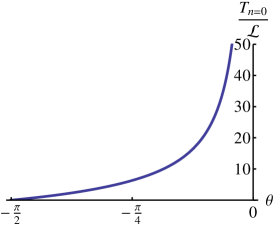
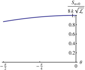
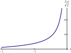
Figure 1: Temperature, entropy and chemical potential of the $n=0$ branch

Inserting this in the second holonomy condition (4.14) gives us a restriction for $C$ given by

$$\sin\left(3C\right)=0,$$ (4.39)

which indicates that $C=n\pi/3$ for $n=0,..,5$. Hence there are six different solutions labelled by $n$. All of these solutions can be regarded as thermodynamical branches of a Lifshitz black hole. The branches $n=1,2,3,4$ all show pathologies that make them unphysical. The $n=1$ case has negative temperature for all values of $\theta,{\mathcal{L}}$, while $n=2$ has both negative temperature and entropy. Finally, the $n=3,4$ branches have strictly negative entropy.

Consequently, only the branches with $n=0$ and $n=5$ seem to be physically sensible. The entropy and temperature of the first brach ($n=0$) read

$$S_{n=0} =8k\sqrt{\cal L}\cos\left(\frac{\theta}{3}\right),\qquad T_{n=0}=-\frac{4{\cal L}}{\sqrt{3}}\frac{\cos\theta}{\sin\frac{\theta}{3}},\qquad\alpha_{n=0}=-2\sqrt{\frac{{\cal L}}{3}}\frac{\cos{\frac{2\theta}{3}}}{\cos{\frac{\theta}{3}}}.$$ (4.40)

This implies that for the temperature to be positive, one needs $-\pi/2<\theta<0$, which imposes the constraint $-\sqrt{16{\cal L}^{3}/27}<{\cal W}<0$. In this range, the entropy has its minimum at zero temperature, in accordance with the third law of thermodynamics. Note that under this constraint, the energy (4.34) is negative, but bounded from below. In section 4.8 we will discuss a simple radial gauge for which this solution looks explicitly like a black hole. Interestingly, this gauge only exists for this branch and $n=4$, which has exactly the same entropy but with the opposite sign. This does not mean that other branches do not have black hole gauges, as we have not explored non-radial gauges. For now, the plots of the temperature and entropy as a function of $\theta$ for a fixed value of ${\mathcal{L}}$, are shown in figure 1.

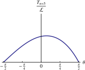
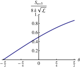
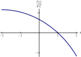
Figure 2: Temperature, entropy and chemical potential of the $n=5$ branch

The sixth branch ($n=5$) shows the following behavior with respect to ${\cal L}$ and $\theta$

$$S_{n=5} =8k\sqrt{\cal L}\cos\left(\frac{\theta+5\pi}{3}\right),\qquad T_{n=5}=\frac{4{\cal L}}{\sqrt{3}}\frac{\cos\theta}{\cos\frac{2\theta+\pi}{6}},\qquad\alpha_{n=5}=2\sqrt{\frac{{\cal L}}{3}}\frac{\cos{\frac{2\theta+\pi}{3}}}{\cos{\frac{2\theta+\pi}{6}}}.$$ (4.41)

This branch has positive values of temperature and entropy for all values of $\theta$, as shown in figure 2.

4.6 Entropy as a function of intensive parameters

Study of the stability and thermodynamical dominance of the different branches requires an expression for the entropy as a function of intensive parameters. This, in turn, requires us to solve the holonomy conditions for ${\cal L,W}$ in terms of $\alpha,T$, and then write the entropy using (4.32) as a function of $\alpha$ and $T$ only. The first holonomy condition (4.13) is linear in ${\cal W}$ and can be easily solved;

$${\mathcal{W}}=-{12\alpha^{2}{\mathcal{L}}+12{\mathcal{L}}^{2}-3T^{2}\over 36\alpha}.$$ (4.42)

Plugging this into the second holonomy condition (4.14), twe obtain the following quartic equation for ${\cal L}$.

$$256{\mathcal{L}}^{4}-576\alpha^{2}{\mathcal{L}}^{3}+(432\alpha^{4}-96\,T^{2}{\mathcal{L}}^{2}+(36\alpha^{2}T^{2}-108\,\alpha^{6}){\mathcal{L}}+27\alpha^{4}T^{2}+9T^{4}=0.$$ (4.43)

This implies the existence of four branches. Even though the number of branches is different from the ones found in last section, one can see that appropriately gluing together these branches, one obtains the solutions we studied in section 4.5. For positive temperature, the only branches with positive entropy can be found in figure 3. Note that branch IV has been plotted for a negative value of $\alpha$ because its entropy is negative otherwise.

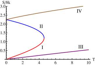
(a) Etropies.

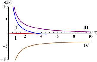
(b) Grand potentials.

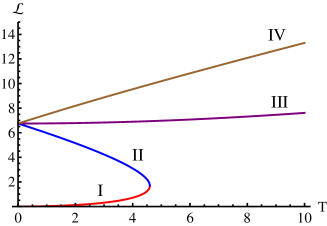
(c) ${\cal L}$ charge.

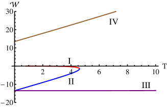
(d) ${\cal W}$ charge.

Figure 3: Entropies, Grand potentials and extensive variables for the four branches as a function of the temperature, at fixed $\alpha$. I,II and III branches have been plotted for $\alpha=3$, while branch IV has $\alpha=-3$

One can check that I and II branches map back to the $n=0$ branch from the previous section, while III and IV are related to the $n=5$ branch. Figure 3(b) shows the grand potential (4.31) as a function of the temperature for fixed chemical potential. In the case of negative $\alpha$, the only sensible branch is IV, and it dominates the thermodynamics. However, for a positive value of $\alpha$, branch I ($n=0$) takes over.

We should note that the phase diagrams displayed in section 4.5 and 4.6 look very similar to the ones obtained for the asymptotically AdS higher spin black holes discussed in [25, 26, 27, 28]. This is no surprise since the holonomy equations are identical. The Lifshitz black hole differs from the AdS higher spin black hole however in the identification of temperature and chemical potential as well as the charges. Hence the physical interpretation of the quantities and physical reasonableness constraints (such as positive temperature) are different.

It is interesting to study the high temperature limit of these solutions. Branch I cannot reach high temperatures at fixed $\alpha$. However, in the high $\alpha$ limit, the temperature can be arbitrarily high at the point of maximum entropy. This point is defined by a concrete value of $\theta$, so the high $\alpha$ limit can only be reached by taking ${\cal L}$ to infinity, as can be seen by looking at equations (4.40). In that case the temperature grows like ${\cal L}$ while the entropy grows like $\sqrt{{\cal L}}$. This implies

$$S_{n=0}\sim\sqrt{T}.$$ (4.44)

The same can be checked for branch IV. In the limit of high temperature, one finds that

$${\cal L} =\frac{\sqrt{3}T}{4}+3^{3/4}\sqrt{\frac{T}{32}}|\alpha|+{\cal O}(1),$$ (4.45)

$$S =-\frac{3^{1/4}\mathrm{sgn}(\alpha)}{\sqrt{8}}\sqrt{T}+{\cal O}(1).$$ (4.46)

Hence for negative $\alpha$ we obtain again

$$S_{n=5}\sim\sqrt{T}.$$ (4.47)

This temperature scaling (4.44) and (4.47) is expected for a theory dual to a quantum field theory with $z=2$ anisotropic Lifshitz scaling symmetry in two dimensions [63].

4.7 Local stability in the grand canonical ensemble

Local thermodynamical stability is associated with the subadditivity of the entropy, as discussed in [60, 61] this condition is equivalent to demanding that the Hessian matrices of $-S$ and $-\beta\Phi$ are positive definite.

$$H_{mn}=\frac{\partial^{2}(-S)}{\partial x_{m}\partial x_{n}},\qquad W_{mn}=\frac{\partial^{2}(-\beta\Phi)}{\partial y_{m}\partial y_{n}}$$ (4.48)

Which Matrix one has to consider depends on whether one describes the thermodynamic state of the system in terms of extensive parameters $x_{i}$ or intensive parameters $y_{i}$ respectively.

In the case of our Lifshitz black hole solution, the extensive parameters can be regarded as the charges $\mathcal{L}$ and $\mathcal{W}$, while the intensive parameters can be regarded as $\beta$ and $\beta\alpha$. Evaluation of the eigenvalues of the Hessian $H_{nm}$ for the $n=5$ branch shows that this condition can’t be satisfied for any value of ${\cal L}$ and ${\cal W}$, so the $n=5$ branch is locally unstable. Demanding positive definiteness of the Hessian for the $n=0$ branch requires that $\theta\in(-3\cos^{-1}\left(\frac{3^{1/4}}{\sqrt{2}}\right),0)$. This is exactly the regime of $\theta$ covered by the curve representing branch I in figure 3.

One can further check that this result is consistent with the description in terms of potentials. Computation of the eigenvalues of $W_{nm}$ for the four branches studied in section 4.6, indeed shows that branch I is locally stable, while II is not.

4.8 Metric and black hole gauge

We now investigate the question whether a gauge exists in which the metric of the Lifshitz black hole solutions displays a regular horizon. In fact, we demonstrate that for some branches one can maintain radial gauge and choose some of the residual gauge such that $g_{tt}$ contains a double zero and $g_{xx}$ is regular.

We begin again with the ansatz (3.9), (3.10) and the flatness conditions (4.4), where again the barred sector is determined by the non-rotating condition $\bar{a}_{x}=-a_{x}^{T}$ and $\bar{a}_{t}=a_{t}^{T}$. We also regard equations (4.5) as a reparametrization of $w_{t,2},l_{t,1},l_{x,-1},$ and $w_{x,-2}$ as functions of the charges and potentials ${\cal L},{\cal W},\mu_{1},\mu_{2},$ and the residual gauge parameter $w_{x,0}$. Next, we solve for the value of $w_{x,0}$ for which the corresponding metric derived from (2.5) has a double zero in $g_{tt}$ at some value of $\rho=\rho_{h}$, the location of the corresponding horizon. To do this, first we note that the metric component $g_{tt}$ can be written as

$$g_{tt}=-(e^{2\rho}p_{1}-e^{-2\rho}p_{2})^{2}-(e^{\rho}p_{3}-e^{-\rho}p_{4})^{2}$$ (4.49)

where $p_{i}$ are $\rho$-independent coefficients given by

$$p_{1} =\mu_{2}$$ (4.50)

$$p_{3} =\mu_{1}-\mu_{2}\frac{w_{x,0}}{3}$$ (4.51)

$$p_{2} =-\left(\frac{w_{x,0}}{3}\right)^{3}\frac{\mu_{1}}{4}+\mathcal{W}\mu_{1}+\mathcal{L}^{2}\mu_{2}+\left(\frac{w_{x,0}}{3}\right)^{4}\frac{\mu_{2}}{16}+\frac{w_{x,0}}{3}2\mathcal{W}\mu_{2}+\frac{1}{2}\mathcal{L}\frac{w_{x,0}}{3}\left(2\mu_{1}+\frac{w_{x,0}}{3}\mu_{2}\right)$$ (4.52)

$$p_{4} =\mathcal{L}\mu_{1}-\left(\frac{w_{x,0}}{3}\right)^{2}\frac{3}{4}\mu_{1}+\frac{w_{x,0}}{3}\mathcal{L}\mu_{2}+\left(\frac{w_{x,0}}{3}\right)^{3}\frac{\mu_{2}}{4}+2\mathcal{W}\mu_{2}$$ (4.53)

It is clear that $g_{tt}$ is zero if and only if each term in parentheses on the right hand side of (4.49) is zero for the same value of $\rho_{h}$ which implies that $p_{2}/p_{1}=(p_{4}/p_{3})^{2}$. Using the expressions above for $p_{1},\dots,p_{4}$, this constraint is equivalent to the following cubic equation for $w_{x,0}$:

$$w_{x,0}^{3}-36\mathcal{L}w_{x,0}-108\mathcal{W}=0.$$ (4.54)

The three solutions are given by

$$w_{x,0}=4\sqrt{3{\cal L}}\cos\left(\frac{\cos^{-1}(\sin\theta)}{3}+m\frac{2\pi}{3}\right),$$ (4.55)

with $m=0,1,2$. However the only solution with a positive and real horizon $\rho_{h}=\sqrt[4]{p_{2}/p_{1}}=\sqrt{p_{4}/p_{3}}$ is the one with $m=2$, which can be simplified to

$$w_{x,0}=-4\sqrt{3{\cal L}}\sin\left(\frac{\theta}{3}\right).$$ (4.56)

The horizon is then located at

$$\rho_{h}=\sqrt{{\cal L}\left(2\cos\frac{2\theta}{3}-1\right)}.$$ (4.57)

It seems that we did not need to impose the holonomy conditions in order to find this black hole gauge. However, we still need to check that the metric and the spin three field in this gauge are smooth around the cycle $t\sim t+2\pi i$. this implies the following conditions

$$1=\sqrt{\frac{g_{tt}}{-2g_{\rho\rho}}}\bigg{|}_{\rho_{h}},\quad\quad 1=\sqrt{\frac{\psi_{xtt}}{-2\psi_{x\rho\rho}}}\bigg{|}_{\rho_{h}}.$$ (4.58)

Direct substitution of the charges and sources for the six branches found in previous sections shows that only the $n=0,3$ cases satisfy these identities. This can mean that this gauge is appropriate for those two solutions, while the other branches require giving up the radial gauge chosen in equation (2.7). As we have argued in section 4.5, the $n=3$ branch does not seem to be physically sensible. For this reason we will focus our attention in branch $n=0$. The values of the spin fields at the horizon in this branch obey the following relations

$$g_{tt}|_{\rho_{h}} =0,\qquad g_{tt}^{\prime}|_{\rho_{h}}=0,\qquad g_{xx}|_{\rho_{h}}=4\mathcal{L},\qquad\psi_{xxx}|_{\rho_{h}}=2\mathcal{W}.$$ (4.59)

So we can recast our expresion for the entropy as

$$S=\frac{4k}{\pi}A\cos\left[\frac{1}{3}\sin^{-1}\left(\frac{3^{\frac{3}{2}}\psi_{3}}{A^{3}}\right)\right]$$ (4.60)

where

$$A =2\pi\sqrt{g_{xx}|_{\rho_{h}}},\qquad\psi_{3}=\psi_{xxx}|_{\rho_{h}},$$ (4.61)

which is very similar to the entropy formula found for asymptotically AdS higher spin black holes [57]. It would be interesting to investigate whether the local thermodynamic instability of the $n=5$ branch discussed in section 4.7 and the absence of a regular horizon are related. However, it is an open and interesting question, if for the $n=5$ branch there is a more general radial gauge choice (along the lines of [21]) which has a regular horizon.

5 Generalizations

In this section we will present some observations on possible generalizations of our $SL(3,\mathbb{R})$ results obtained in the previous sections.

5.1 Rotating solutions

In the present paper we have limited ourselves to non-rotating solutions, for which the connections $A$ and $\bar{A}$ are related by equation (4.1). Since the two Chern-Simons connections $A,\bar{A}$ are independent, it is clear that constructing a solution with angular momentum entails lifting the condition (4.1). This also means that there will be two holonomy conditions for the $A$ and the $\bar{A}$ connection. Recall that in the $SL(3,\mathbb{R})\times SL(3,\mathbb{R})$ black hole first discussed in [24] a rotating higher spin black hole is obtained by choosing modular parameter to be complex $\tau=\Omega+i\beta$, where $\Omega$ is the potential dual to the angular momentum. For the Lifshitz black holes this cannot work quite the same way and we present some observations here. Note that in the holographic dictionary or the stress energy complex of a Lifshitz theory (5.1) the angular momentum (i.e. the momentum along the $x$ direction if we take $x$ to be compact) is identified with ${\mathcal{L}}-\bar{\mathcal{L}}$, whose conjugate potential is $\mu_{1}-\bar{\mu}_{1}$ and the energy is identified with ${\mathcal{W}}+\bar{\mathcal{W}}$, whose conjugate potential is $\mu_{2}+\bar{\mu}_{2}$. Hence it is likely that a rotating solution can be constructed by choosing a connections with $\mu_{1}\neq\bar{\mu}_{1}$ and keeping the indentification of the temperature $\beta$ the same as in the non-rotating case. The expressions for the metric and higher spin fields are much more complicated. This implies also that the analysis of the black hole gauge done section 4.8 becomes more involved, and we leave these questions for future work. We also note that, to our knowledge, no rotating Lifshitz black hole solutions have been constructed using the standard supergravity actions. Hence constructing such solutions in higher spin gravity might be interesting.

5.2 Lifshitz vacuum for $hs(\lambda)$

In this section we discuss some steps in generalizing the construction of Lifshitz black holes from $SL(3,\mathbb{R})$ to $hs(\lambda)$, note that this generalization will also include the case of $SL(N,\mathbb{R})$ by choosing $\lambda=N$, where the infinite-dimensional Lie algebra reduces to $SL(N,\mathbb{R})$. Our conventions for $hs(\lambda)$ are summarized in appendix A.2.

A Lifshitz vacuum in the $hs(\lambda)$ theory can be easily constructed as follows

$$a_{t} ={1\over\sqrt{\operatorname{tr}(V^{s}_{s-1}V^{s}_{-(s-1)})}}V^{s}_{s-1}, a_{x} ={1\over\sqrt{\operatorname{tr}(V^{2}_{1}V^{2}_{-1})}}V_{1}^{2}$$

$$\bar{a}_{t} ={1\over\sqrt{\operatorname{tr}(V^{s}_{s-1}V^{s}_{-(s-1)})}}V^{s}_{-(s-1)}, \bar{a}_{x} =-{1\over\sqrt{\operatorname{tr}(V^{2}_{1}V^{2}_{-1})}}V_{-1}^{2}.$$ (5.1)

Note that since

$$[V_{1}^{2},V^{s}_{s-1}]_{\star}=0,\quad\quad[V_{-1}^{2},V^{s}_{-(s-1)}]_{\star}=0,$$ (5.2)

this satisfies the flatness condition for a connection in the radial gauge. The gauge connections $A_{\mu}$ and the metric are obtained from (5.2) by adapting the formulae (2.5) and using $b=\exp(\rho V^{2}_{0})$ It follows that the metric is of the form.

$$ds^{2}=-e^{2(s-1)\rho}dt^{2}+e^{2\rho}dx^{2}+d\rho^{2}.$$ (5.3)

Hence we can realize an asymptotically Lifshitz metric in the $hs(\lambda)$ theory for any $z=2,3,4,\cdots$, by setting $s=z+1$. Note that some higher spin fields will be non-vanishing for this $hs(\lambda)$ Lifshitz vacuum. By setting $\lambda=N$, the infinite-dimensional $hs(\lambda)$ gauge algebra truncates to a finite-dimensional $SL(N,\mathbb{R})$, and the connections give Lifshitz vacua with $z=N-1,N-2,\cdots,2$.

5.3 An $hs(\lambda)$ Lifshitz black hole

Here we limit ourself to the BH for $z=2$, which is related to the $hs(\lambda)$ black hole with a chemical potential for the spin three charge, which is most extensively studied in the literature. The connection is given by

$$a_{x} =V_{1}^{2}+\tilde{\mathcal{L}}V_{-1}^{2}+\tilde{\mathcal{W}}V_{-2}^{3}+\tilde{\mathcal{U}}V_{-3}^{4}+\cdots$$ (5.4)

$$a_{t} =\tilde{\mu}_{1}a_{x}+\tilde{\mu}_{2}(a_{x}\star a_{x})\mid_{\rm traceless}.$$ (5.5)

Here, $\tilde{\mathcal{L}},\tilde{\mathcal{W}},\tilde{\mathcal{U}}$, etc are associated with charges of spin $2,3,4,\cdots$. We have tilded all quantities to distinguish them from the quantities appearing in the higher spin black hole reviewed in the appendix A.2.

By construction the connection (5.4) satisfied the flatness condition. To define a regular black hole in a higher spin Chern-Simons theory one has to impose a holonomy condition on the gauge connection around the euclidean time circle. The holonomy condition which we choose is again that the holonomy is equal to the BTZ holonomy for the $hs(\lambda)$ black hole defined in appendix A.2. One might object that in the case of the Lifshitz BH this condition seems less well motivated since there is no analog of a BTZ black hole for an asymptotically Lifshitz spacetime, however a better way to think about this is that the BTZ holonomy simply states that the holonomy of the BH is in the center of $hs(\lambda)$ (see Gaberdiel:2013jca for a discussion on how the center of $hs(\lambda)$ is defined).

If we compare the holonomy associated with $a_{t}$ defined in (5.4) and the higher spin black hole holonomy (A.17) one recognizes that they are the same upon the following identifications

$$\tilde{\mu}_{1}=2\pi\tau,\quad\quad\tilde{\mu}_{2}=-2\pi\alpha.$$ (5.6)

Furthermore the charges can also be identified

$$\tilde{\mathcal{L}}=-{2\pi\over k}{\mathcal{L}},\quad\quad\tilde{\mathcal{W}}=-{\pi\over 2k}{\mathcal{W}},\quad\cdots$$ (5.7)

Since there is a one-to-one map of parameters one might ask how this can be different than the $hs(\lambda)$ [56]. The answer lies in the fact that while (this was true for the $SL(3,\mathbb{R})$ case too) the holonomy conditions have the same functional form, the interpretations of $\tilde{\mu}_{1}$ and $\tilde{\mu}_{2}$ are different. The inverse temperature $\beta$ and the chemical potential $\tilde{\alpha}$ can be related to $\tilde{\mu}_{1}$ and $\tilde{\mu}_{2}$ following the the $SL(3,\mathbb{R})$ Lifshitz black hole example

$$\tilde{\mu}_{1}=\beta\tilde{\alpha},\quad\quad\tilde{\mu}_{2}=\beta.$$ (5.8)

This means that the most natural regime for the Lifshitz black hole , i.e. $\tilde{\beta}$ finite and $\tilde{\alpha}$ small, is not the same regime as the one which allows the perturbative solution of the holonomy conditions first obtained in [56]. Indeed if we take the limit $\tilde{\alpha}\to 0$, this is equivalent for the higher spin black hole to taking the limit $\tau\to 0$ and keeping $\alpha$ finite, i.e. taking an infinite temperature limit and finite chemical potential.

6 Discussion

In this paper we have discussed the construction of holographic spacetimes dual to field theory with Lifshitz $z=2$ scaling symmetry . In addition we have constructed black hole solutions in these theories. One interesting feature of these theories is that the connections, holonomy conditions and thermodynamic relations are all very similar to the higher spin black holes first constructed in [24]. This can be traced back to the fact that the Lifshitz black hole connections and the higher spin black hole connections are related by replacing $t,x$ by $\bar{z},z$ respectively. Note however that the interpretation of the parameters is quite different. First, the holographic identification of the stress energy complex of the QFT with Lifshitz symmetry and the role of the fields ${\mathcal{L}}$ and ${\mathcal{W}}$ are quite different for the Lifshitz theory compared to the $W_{3}$ CFT. Second, for the Lifshitz black hole solutions the identification of the temperature and higher spin chemical potential is in some sense reversed compared to the higher spin black hole, this leads to a different interpretation of the thermodynamics. The solution of the holonomy conditions has different branches, which we can interpret as different thermodynamic phases. We have shown that only one branch (branch I of section 4.6) has 1. positive entropy and 2. positive temperature, 3. is locally thermodynamically stable and 4. enjoys a radial gauge with a regular horizon. All other branches do not satisfy one or more of these conditions and are therefore physically not satisfying.

We have briefly discussed generalizations of the black hole solutions found in this paper. It would be interesting to study Lifshitz black hole solutions in $hs(\lambda)$ further, since there exists a concrete proposal for a dual CFT and the Lifshitz theories could be interpreted as deformations of the CFT. Furthermore since it is possible to couple scalar matter consistently there are independent probes of the geometry of the black hole. To make progress one has to solve the holonomy conditions either exactly or maybe less ambitiously determine wether it is possible to solve the holonomy conditions perturbatively for small $\tilde{\alpha}$ and finite temperature. We plan to return to these interesting questions in the future.

Acknowledgements

This work was in part supported by NSF grant PHY-07-57702 and PHY-13-13986. M.G. is grateful to the Centro de Ciencias de Benasque Pedro Pascual for hospitality while this work was in progress. M.G. is gratefu for hospitality at the Institute of Theoretical Physics, University of Jena while this paper was finalized. E.H. acknowledges support from Fundación la Caixa. We are grateful to Martin Ammon, Per Kraus, Edgar Shaghoulian, and Arnaud Lepage-Jutier for useful conversations.

Appendix A Conventions

In this appendix we present some details on the conventions and explicit representations of the Lie algebras used in the main body of the paper.

A.1 Explicit $SL(3,\mathbb{R})$ representation

The $SL(2,\mathbb{R})$ generators of the principal embedding are given by the following matrices

$$L_{-1}=\begin{pmatrix}0&\sqrt{2}&0\\ 0&0&\sqrt{2}\\ 0&0&0\\ \end{pmatrix},\qquad L_{1}=\begin{pmatrix}0&0&0\\ -\sqrt{2}&0&0\\ 0&-\sqrt{2}&0\\ \end{pmatrix},\qquad L_{0}=\begin{pmatrix}1&0&0\\ 0&0&0\\ 0&0&-1\\ \end{pmatrix}.$$ (A.1)

and the spin 3 generators, on which we omit the superscript ⁽³⁾ for notational simplicity, are as follows:

$$W_{-2} =\begin{pmatrix}0&0&2\\ 0&0&0\\ 0&0&0\\ \end{pmatrix},\qquad W_{-1}=\begin{pmatrix}0&\frac{1}{\sqrt{2}}&0\\ 0&0&-\frac{1}{\sqrt{2}}\\ 0&0&0\\ \end{pmatrix},\qquad W_{0}=\begin{pmatrix}\frac{1}{3}&0&0\\ 0&-\frac{2}{3}&0\\ 0&0&\frac{1}{3}\\ \end{pmatrix}$$ (A.2)

$$W_{1} =\begin{pmatrix}0&0&0\\ -\frac{1}{\sqrt{2}}&0&0\\ 0&\frac{1}{\sqrt{2}}&0\\ \end{pmatrix},\qquad W_{2}=\begin{pmatrix}0&0&0\\ 0&0&0\\ 2&0&0\\ \end{pmatrix}.$$ (A.3)

If we define $(T_{1},T_{2},\dots,T_{8})=(L_{1},L_{0},L_{-1},W_{2},\dots W_{-2})$, then traces of all pairs of generators are given by

$$\mathrm{tr}(T_{i}T_{j}) =\left(\begin{array}[]{ccc|ccccc}&&-4&0&&\cdots&&0\\ &2&&\vdots&&\ddots&&\vdots\\ -4&&&0&&\cdots&&0\\ \hline\cr 0&\cdots&0&&&&&4\\ &&&&&&-1&\\ \vdots&\ddots&\vdots&&&\frac{2}{3}&&\\ &&&&-1&&&\\ 0&\cdots&0&4&&&&\end{array}\right)$$ (A.12)

A.2 $hs(\lambda)$ conventions and black hole

Here we follow the conventions of [29] and [31]. The main formulas we use are, the lone star products

$$V_{m}^{s}\star V_{n}^{t}={1\over 2}\sum_{u}{1,2,\cdots}^{s+t-|s-t|-1}g_{u}^{st}(m,n;\lambda)V_{m+n}^{s+t-u}.$$ (A.13)

The star product is used to define the commutator between Lie algebra generator and is denotes by $[\cdot,\cdot]_{\star}$. For the elements of the Lie-algebra $V^{s}_{m}$ one has $|m|<s$ (the generators are zero otherwise). The elements $V^{2}_{-1,0,1}$ form a SL(2,R) sub algebra and $V^{s}_{m}$ form spin s representation

$$[V_{m}^{2},V_{n}^{t}]_{*}=\Big{(}m(t-1)-n\Big{)}V_{m+n}^{t}.$$ (A.14)

The algebra has a unit element denoted by $X^{1}_{0}$, the trace is defines by

$$Tr(X)=X{\mid}{}_{V^{1}_{0}}.$$ (A.15)

A $hs(\lambda)$ black hole with a chemical potential for the spin 3 charge (this can be generalized to arbitrary spin $s$) has the following connections

$$a_{z} =V_{1}^{2}-{2\pi\over k}{\mathcal{L}}V_{-1}^{2}-{\pi\over 2k}{\mathcal{W}}V_{-2}^{3}+{\mathcal{U}}V_{-3}^{4}+\cdots,$$

$$a_{\bar{z}} =-{\alpha\over\bar{\tau}}(a_{z}\star a_{z})\mid_{\rm traceless}.$$ (A.16)

The holonomy around the time circle is given by $H=e^{\omega}$ with

$$\omega=2\pi\big{(}\tau a_{z}+\bar{\tau}a_{\bar{z}}\big{)}.$$ (A.17)

The holonomy condition for the black hole is that the holonomy is the same as the holonomy of the BTZ black hole

$$H=H_{BTZ}.$$ (A.18)

where $\omega_{BTZ}$ is given by

$$\omega_{BTZ}=2\pi\tau V_{1}^{2}+{\pi\over\tau}V_{-1}^{2}.$$ (A.19)

This condition is equivalent to the following conditions on the powers of $\omega$ (see eq. 2.17 of [31]).

$$Tr(\omega^{n})={1\over\lambda}\lim_{t\to 0}\left(\partial_{t}^{n}{\sin\pi\lambda t\over\sin\pi t}\right).$$ (A.20)

These conditions have been solved perturbatively in the chemical potential $\alpha$ and one gets the charges ${\mathcal{L}},{\mathcal{W}},{\mathcal{U}},\cdots$ as a power series in $\alpha$ (and depending on $\tau$), such that as $\alpha\to 0$ one gets back the BTZ black hole.

References

- [1]
- [2] M. A. Vasiliev, “Higher spin symmetries, star product and relativistic equations in AdS space,” hep-th/0002183.
- [3] M. R. Gaberdiel and R. Gopakumar, “An AdS3 Dual for Minimal Model CFTs,” Phys. Rev. D 83 (2011) 066007 [arXiv:1011.2986 [hep-th]].
- [4] E. Witten, “(2+1)-Dimensional Gravity as an Exactly Soluble System,” Nucl. Phys. B 311 (1988) 46.
- [5] A. Achucarro and P. K. Townsend, “A Chern-Simons Action for Three-Dimensional anti-De Sitter Supergravity Theories,” Phys. Lett. B 180 (1986) 89.
- [6] M. R. Gaberdiel and T. Hartman, “Symmetries of Holographic Minimal Models,” JHEP 1105 (2011) 031 [arXiv:1101.2910 [hep-th]].
- [7] M. R. Gaberdiel, R. Gopakumar, T. Hartman and S. Raju, “Partition Functions of Holographic Minimal Models,” JHEP 1108 (2011) 077 [arXiv:1106.1897 [hep-th]].
- [8] M. R. Gaberdiel and R. Gopakumar, “Triality in Minimal Model Holography,” JHEP 1207 (2012) 127 [arXiv:1205.2472 [hep-th]].
- [9] A. Castro, R. Gopakumar, M. Gutperle and J. Raeymaekers, “Conical Defects in Higher Spin Theories,” JHEP 1202 (2012) 096 [arXiv:1111.3381 [hep-th]].
- [10] C. -M. Chang and X. Yin, “Higher Spin Gravity with Matter in AdS3 and Its CFT Dual,” JHEP 1210 (2012) 024 [arXiv:1106.2580 [hep-th]].
- [11] M. Ammon, P. Kraus and E. Perlmutter, “Scalar fields and three-point functions in D=3 higher spin gravity,” JHEP 1207 (2012) 113 [arXiv:1111.3926 [hep-th]].
- [12] E. Perlmutter, T. Prochazka and J. Raeymaekers, “The semiclassical limit of CFTs and Vasiliev theory,” JHEP 1305 (2013) 007 [arXiv:1210.8452 [hep-th]].
- [13] E. Hijano, P. Kraus and E. Perlmutter, “Matching four-point functions in higher spin AdS3/CFT2,” JHEP 1305 (2013) 163 [arXiv:1302.6113 [hep-th]].
- [14] S. F. Prokushkin and M. A. Vasiliev, “Higher spin gauge interactions for massive matter fields in 3-D AdS spacetime,” Nucl. Phys. B 545 (1999) 385 [hep-th/9806236].
- [15] M. P. Blencowe, “A Consistent Interacting Massless Higher Spin Field Theory In D = (2+1),” Class. Quant. Grav. 6 (1989) 443.
- [16] E. Bergshoeff, M. P. Blencowe and K. S. Stelle, “Area Preserving Diffeomorphisms And Higher Spin Algebra,” Commun. Math. Phys. 128 (1990) 213.
- [17] C. N. Pope, L. J. Romans and X. Shen, “W(infinity) And The Racah-wigner Algebra,” Nucl. Phys. B 339 (1990) 191.
- [18] A. Campoleoni, S. Fredenhagen, S. Pfenninger and S. Theisen, “Asymptotic symmetries of three-dimensional gravity coupled to higher-spin fields,” JHEP 1011 (2010) 007 [arXiv:1008.4744 [hep-th]].
- [19] M. Henneaux and S. -J. Rey, “Nonlinear as Asymptotic Symmetry of Three-Dimensional Higher Spin Anti-de Sitter Gravity,” JHEP 1012 (2010) 007 [arXiv:1008.4579 [hep-th]].
- [20] A. Campoleoni, S. Fredenhagen and S. Pfenninger, “Asymptotic W-symmetries in three-dimensional higher-spin gauge theories,” JHEP 1109 (2011) 113 [arXiv:1107.0290 [hep-th]].
- [21] M. Ammon, M. Gutperle, P. Kraus and E. Perlmutter, “Spacetime Geometry in Higher Spin Gravity,” JHEP 1110 (2011) 053 [arXiv:1106.4788 [hep-th]].
- [22] M. Banados, C. Teitelboim and J. Zanelli, “The Black hole in three-dimensional spacetime,” Phys. Rev. Lett. 69 (1992) 1849 [hep-th/9204099].
- [23] P. Kraus, “Lectures on black holes and the AdS(3) / CFT(2) correspondence,” Lect. Notes Phys. 755 (2008) 193 [hep-th/0609074].
- [24] M. Gutperle and P. Kraus, “Higher Spin Black Holes,” JHEP 1105 (2011) 022 [arXiv:1103.4304 [hep-th]].
- [25] A. Castro, E. Hijano, A. Lepage-Jutier and A. Maloney, “Black Holes and Singularity Resolution in Higher Spin Gravity,” JHEP 1201 (2012) 031 [arXiv:1110.4117 [hep-th]].
- [26] J. R. David, M. Ferlaino and S. P. Kumar, “Thermodynamics of higher spin black holes in 3D,” JHEP 1211 (2012) 135 [arXiv:1210.0284 [hep-th]].
- [27] B. Chen, J. Long and Y. -n. Wang, “Black holes in Truncated Higher Spin AdS3 Gravity,” JHEP 1212 (2012) 052 [arXiv:1209.6185 [hep-th]].
- [28] B. Chen, J. Long and Y. -N. Wang, “Phase Structure of Higher Spin Black Hole,” JHEP 1303 (2013) 017 [arXiv:1212.6593].
- [29] P. Kraus and E. Perlmutter, “Probing higher spin black holes,” JHEP 1302 (2013) 096 [arXiv:1209.4937 [hep-th]].
- [30] M. R. Gaberdiel, T. Hartman and K. Jin, “Higher Spin Black Holes from CFT,” JHEP 1204 (2012) 103 [arXiv:1203.0015 [hep-th]].
- [31] M. R. Gaberdiel, K. Jin and E. Perlmutter, “Probing higher spin black holes from CFT,” arXiv:1307.2221 [hep-th].
- [32] M. Ammon, M. Gutperle, P. Kraus and E. Perlmutter, “Black holes in three dimensional higher spin gravity: A review,” J. Phys. A 46 (2013) 214001 [arXiv:1208.5182 [hep-th]].
- [33] A. Perez, D. Tempo and R. Troncoso, “Higher spin gravity in 3D: black holes, global charges and thermodynamics,” arXiv:1207.2844 [hep-th].
- [34] J. de Boer and J. I. Jottar, “Thermodynamics of Higher Spin Black Holes in AdS3,” arXiv:1302.0816 [hep-th].
- [35] A. Perez, D. Tempo and R. Troncoso, “Higher spin black hole entropy in three dimensions,” arXiv:1301.0847 [hep-th].
- [36] P. Kraus and T. Ugajin, “An Entropy Formula for Higher Spin Black Holes via Conical Singularities,” JHEP 1305 (2013) 160 [arXiv:1302.1583 [hep-th]].
- [37] J. de Boer and J. I. Jottar, “Entanglement Entropy and Higher Spin Holography in AdS3,” arXiv:1306.4347 [hep-th].
- [38] M. Ammon, A. Castro and N. Iqbal, “Wilson Lines and Entanglement Entropy in Higher Spin Gravity,” arXiv:1306.4338 [hep-th].
- [39] M. Gary, D. Grumiller and R. Rashkov, “Towards non-AdS holography in 3-dimensional higher spin gravity,” JHEP 1203 (2012) 022 [arXiv:1201.0013 [hep-th]].
- [40] H. Afshar, M. Gary, D. Grumiller, R. Rashkov and M. Riegler, “Non-AdS holography in 3-dimensional higher spin gravity - General recipe and example,” JHEP 1211 (2012) 099 [arXiv:1209.2860 [hep-th]].
- [41] H. Afshar, A. Bagchi, R. Fareghbal, D. Grumiller and J. Rosseel, “Higher spin theory in 3-dimensional flat space,” arXiv:1307.4768 [hep-th].
- [42] H. A. Gonzalez, J. Matulich, M. Pino and R. Troncoso, “Asymptotically flat spacetimes in three-dimensional higher spin gravity,” arXiv:1307.5651 [hep-th].
- [43] S. Kachru, X. Liu and M. Mulligan, “Gravity Duals of Lifshitz-like Fixed Points,” Phys. Rev. D 78 (2008) 106005 [arXiv:0808.1725 [hep-th]].
- [44] A. Donos and J. P. Gauntlett, “Supersymmetric solutions for non-relativistic holography,” JHEP 0903 (2009) 138 [arXiv:0901.0818 [hep-th]].
- [45] K. Balasubramanian and K. Narayan, “Lifshitz spacetimes from AdS null and cosmological solutions,” JHEP 1008 (2010) 014 [arXiv:1005.3291 [hep-th]].
- [46] A. Donos and J. P. Gauntlett, “Lifshitz Solutions of D=10 and D=11 supergravity,” JHEP 1012 (2010) 002 [arXiv:1008.2062 [hep-th]].
- [47] R. Gregory, S. L. Parameswaran, G. Tasinato and I. Zavala, “Lifshitz solutions in supergravity and string theory,” JHEP 1012 (2010) 047 [arXiv:1009.3445 [hep-th]].
- [48] U. H. Danielsson and L. Thorlacius, “Black holes in asymptotically Lifshitz spacetime,” JHEP 0903 (2009) 070 [arXiv:0812.5088 [hep-th]].
- [49] G. Bertoldi, B. A. Burrington and A. Peet, “Black Holes in asymptotically Lifshitz spacetimes with arbitrary critical exponent,” Phys. Rev. D 80 (2009) 126003 [arXiv:0905.3183 [hep-th]].
- [50] R. B. Mann, “Lifshitz Topological Black Holes,” JHEP 0906 (2009) 075 [arXiv:0905.1136 [hep-th]].
- [51] K. Balasubramanian and J. McGreevy, “An Analytic Lifshitz black hole,” Phys. Rev. D 80 (2009) 104039 [arXiv:0909.0263 [hep-th]].
- [52] M. Henneaux, A. Perez, D. Tempo and R. Troncoso, “Chemical potentials in three-dimensional higher spin anti-de Sitter gravity,” arXiv:1309.4362 [hep-th].
- [53] S. F. Ross, “Holography for asymptotically locally Lifshitz spacetimes,” Class. Quant. Grav. 28 (2011) 215019 [arXiv:1107.4451 [hep-th]].
- [54] G. Compere, S. de Buyl, S. Detournay and K. Yoshida, “Asymptotic symmetries of Schrodinger spacetimes,” JHEP 0910 (2009) 032 [arXiv:0908.1402 [hep-th]].
- [55] M. Banados, R. Canto and S. Theisen, “The Action for higher spin black holes in three dimensions,” JHEP 1207 (2012) 147 [arXiv:1204.5105 [hep-th]].
- [56] P. Kraus and E. Perlmutter, “Partition functions of higher spin black holes and their CFT duals,” JHEP 1111 (2011) 061 [arXiv:1108.2567 [hep-th]].
- [57] A. Pérez, D. Tempo and R. Troncoso , “Higher spin black hole entropy in three dimensions,” [arXiv:1301.0847 [hep-th]].
- [58] D.C. Wright, “Black holes and the Gibbs-Duhem relation,” Phys. Rev. D 21 (1980) 884–890
- [59] G. W. Gibbons, M. J. Perry and C. N. Pope, “The First law of thermodynamics for Kerr-anti-de Sitter black holes,” Class. Quant. Grav. 22 (2005) 1503 [hep-th/0408217].
- [60] S. S. Gubser and I. Mitra, “The Evolution of unstable black holes in anti-de Sitter space,” JHEP 0108 (2001) 018 [hep-th/0011127].
- [61] R. J. F. Monteiro, “Classical and thermodynamic stability of black holes,” [hep-th/1006.5358].
- [62] M. Banados, “Global charges in Chern-Simons field theory and the (2+1) black hole,” Phys. Rev. D 52, 5816 (1996) [hep-th/9405171].
- [63] H. A. Gonzalez, D. Tempo and R. Troncoso, “Field theories with anisotropic scaling in 2D, solitons and the microscopic entropy of asymptotically Lifshitz black holes,” JHEP 1111 (2011) 066 [arXiv:1107.3647 [hep-th]].
- [64]