Diffusion, subdiffusion, and trapping of active particles in heterogeneous media

Abstract

We study the transport properties of a system of active particles moving at constant speed in an heterogeneous two-dimensional space. The spatial heterogeneity is modeled by a random distribution of obstacles, which the active particles avoid. Obstacle avoidance is characterized by the particle turning speed $\gamma$. We show, through simulations and analytical calculations, that the mean square displacement of particles exhibits two regimes as function of the density of obstacles $\rho_{o}$ and $\gamma$. We find that at low values of $\gamma$, particle motion is diffusive and characterized by a diffusion coefficient that displays a minimum at an intermediate obstacle density $\rho_{o}$. We observe that in high obstacle density regions and for large $\gamma$ values, spontaneous trapping of active particles occurs. We show that such trapping leads to genuine subdiffusive motion of the active particles. We indicate how these findings can be used to fabricate a filter of active particles.

Locomotion patterns are of prime importance for the survival of most organisms at all scales, ranging from bacteria to birds, and often involving complex processes that require energy consumption: i.e. the active motion of the organism Berg (1983); Okubo and Levin (1980). The characterization and study of these patterns have a long tradition Berg (1983); Okubo and Levin (1980) and the experimental observation of subdiffusion, diffusion, and superdiffusion has motivated the development of powerful theoretical tools Metzler and Klafter (2000). It is only in recent years that the (thermodynamical) non-equilibrium nature of these active patterns has been exploited, leading to the study of the so-called active particle systems romanczuk2012 . Exciting non-equilibrium features have been reported in both, interacting as well as non-interacting active particle systems. For instance, large-scale collective motion and giant number fluctuations have been found in interacting active particle systems Vicsek and Zafeiris (2012); Ramaswamy (2010); ginelli2010 ; peruani2012 . In non-interacting active particle systems, the presence of active fluctuations leads to complex, non-equilibrium transients in the particle mean square displacement Peruani and Morelli (2007); Golestanian (2009) and anomalous velocity distributions Romanczuk and Schimansky-Geier (2011), and the lack of momentum conservation induces non-classical particle-wall interactions, which allows, for instance, the rectification of particle motion galajda2007 ; Wensink and Löwen (2008); wan2008 ; Tailleur and Cates (2009); Radtke and Schimansky-Geier (2012).

The study of active particle systems has recently witnessed the emergence of a promising new direction: the design and construction of biomimetic, artificial active particles. The directed driving is usually obtained by fabricating asymmetric particles that possess two distinct friction coefficients Kudrolli et al. (2006); Deseigne et al. (2010); weber2013 , light absorption coefficients Jiang et al. (2010); Golestanian (2012); theurkauff2012 ; palacci2013 , or catalytic properties et al. (2004); Mano and Heller (2005); Rückner and Kapral (2007); howse2007 ; R. Golestanian and Ajdari (2005); Golestanian (2009) depending on whether energy injection is done through vibration, light emission, or chemical reaction, respectively. One of the most prominent features of these artificial active particles is that their motion is characterized by a diffusion coefficient remarkably larger than the one obtained using symmetric particles Golestanian (2009).

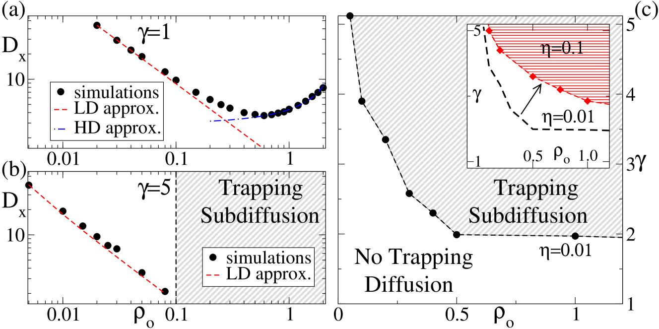
Figure 1: Diffusive and subdiffusive regimes. (a) For low values of the turning speed $\gamma$, the motion is diffusive and characterized by a diffusion coefficient $D_{x}$ that exhibits a minimum with the obstacle density $\rho_{o}$, as expected by combining the low-density (LD) and high-density (HD) approximation. See Eq. (9), (11) and text. (b) For large values of $\gamma$, diffusive motion occurs at low $\rho_{o}$ values only, while for large $\rho_{o}$ values, particle motion becomes subdiffusive. (c) The boundary between the diffusive and subdiffusive regime is given, for a fixed noise $\eta$, by $\rho_{o}$ and $\gamma$, see inset and boundaryEstimate . Parameters: $R=1$, $L=100$, $N_{p}=10^{4}$, and $\eta=0.01$ (inset in (c), $\eta=0.1$).

The rapidly expanding study of active particles has focused so far almost exclusively, theoretically as well as experimentally, on the statistical description of particle motion in idealized, homogeneous spaces. However, the great majority of natural active particle systems takes place, in the wild, in heterogeneous media: from active transport inside the cell, which occurs in a space that is filled by organelles and vesicles alberts , to bacterial motion, which takes place in highly heterogeneous environments such as the soil or complex tissues such as in the gastrointestinal tract Dworkin (1993). While diffusion in random media is a well studied subject Bouchaud and Geoges (1990); Berry and Chaté (2011), the impact that an heterogeneous medium may have on the locomotion patterns of active particles remains poorly explored.

We address this fundamental problem by using a simple model in which the active organisms move at constant speed in an heterogeneous two-dimensional space, where the heterogeneity is given by a random distribution of obstacles. An “obstacle” may represent the source of a repellent chemical, a light gradient, a burning spot in a forest, or whatever threat that makes our (self-propelled) organisms to move away from it once the danger has been sensed; with obstacle avoidance characterized by a (maximum) turning speed $\gamma$. Our analysis shows that the same evolution equations (behavioral rules) lead to very different locomotion patterns at low and high density of obstacles. In the dilute obstacle scenario, there is no conflicting information and organisms can easily move away from the undesirable area they find in their way. On the other hand, when we stress the environmental conditions, such that organisms sense several repellent sources simultaneously, the processing of the information is no longer simple. Organisms compute the local obstacle density gradient and use this information to move away from higher obstacle densities. Since the distribution of obstacles is random, as the overall obstacle density increases, this task becomes increasingly more difficult. As result of this, no strategy guaranties how to escape away from obstacles and the organisms behave more and more as if there were no obstacles in the system. For low $\gamma$ values, we find that the above described change of behavior is reflected by the minimum exhibited by the diffusion coefficient at intermediate obstacle densities $\rho_{o}$, Fig. 1(a). For large $\gamma$ values, particle motion is diffusive at small densities $\rho_{o}$, while for large enough densities a new phenomenon emerges: spontaneous trapping of particles, Fig. 1(b). These traps are closed orbits found by the particles in a landscape of obstacles, Fig. 2. The time particles spend in these orbits is heavy-tailed distributed, and particle motion is genuinely (i.e., asymptotically) subdiffusive. The boundary between the diffusive and subdiffusive regime depends on $\gamma$ and $\rho_{o}$ as illustrated in Fig. 1(c).

Our results open a new route to control active particle systems. For instance, the appearance of spontaneous trapping as a dynamical phenomenon that depends on the intrinsic properties of the particles allows us to design a generic filter of active particles.

Model definition.– We consider a continuum time model for $N_{p}$ self-propelled particles moving in a two-dimensional space of linear size $L$ where $N_{o}$ obstacles are placed at random commentUS . Boundary conditions are periodic. In the over-damped limit, the equations of motion of the $i$-th particle are given by:

$$\dot{\mathbf{x}}_{i} = v_{0}\mathbf{V}(\theta_{i})$$ (1)

$$\dot{\theta}_{i} = h(\mathbf{x}_{i})+\eta\xi_{i}(t)\,,$$ (2)

where the dot denotes temporal derivative, $\mathbf{x}_{i}$ corresponds to the position of the $i$-th particle, and $\theta_{i}$ to its moving direction. The function $h(\mathbf{x}_{i})$ represents the interaction with obstacles and its definition is given by:

$$h(\mathbf{x}_{i})=\begin{cases}\frac{\gamma}{n(\mathbf{x}_{i})}\sum_{\Omega_{i}}\sin(\alpha_{k,i}-\theta_{i})&\text{if }n(\mathbf{x}_{i})>0\\ 0&\text{if }n(\mathbf{x}_{i})=0\,,\end{cases}$$ (3)

where the sum runs over all neighboring obstacles $\Omega_{i}$ such that $0<|\mathbf{x}_{i}-\mathbf{y}_{k}|<R$, with $\mathbf{y}_{k}$ the position of the $k$-th obstacle, and the term $\alpha_{k,i}$ the angle, in polar coordinates, of the vector $\mathbf{x}_{i}-\mathbf{y}_{k}$. The term $n(\mathbf{x}_{i})$ denotes the number of obstacles located at a distance less or equal than $R$ from $\mathbf{x}_{i}$. In Eq. (1), $v_{\rm 0}$ is the active particle speed and $\mathbf{V}(\theta)\equiv(\cos(\theta),\sin(\theta))^{T}$. The additive white noise in Eq. (2) is characterized by an amplitude $\eta$ and obeys $\langle\xi_{i}(t)\rangle=0$ and $\langle\xi_{i}(t)\xi_{j}(t^{\prime})\rangle=\delta_{i,j}\delta(t-t^{\prime})$, which leads to an angular diffusion $D_{\theta}=\eta^{2}/2$. Notice that for $\gamma=0$, equations (1) and (2) define a system of persistent random walkers characterized by a diffusion coefficient $D_{x_{o}}=v_{0}^{2}/(2D_{\theta})$, see Berg (1983); Okubo and Levin (1980); Peruani and Morelli (2007).

Continuum description.– We look for a coarse-grain description of the system in terms of the concentration $p(\mathbf{x},\theta,t)$ of particles at position $\mathbf{x}$ and orientation $\theta$ at time $t$. The evolution of $p(\mathbf{x},\theta,t)$ obeys gardiner :

$$\partial_{t}p+v_{0}\nabla.\left[\mathbf{V}(\theta)p\right]=D_{\theta}\partial_{\theta\theta}p+F[p(\mathbf{x},\theta,t),\rho_{o}(\mathbf{x})]\,,$$ (4)

where $D_{\theta}$ is the angular diffusion as defined above, and $F[p(\mathbf{x},\theta,t),\rho_{o}(x)]$ represents the interaction of the self-propelled particles with the obstacles. The term $\rho_{o}(\mathbf{x})$ refers to the obstacle density at position $\mathbf{x}$ comment0 . Here, we discuss two clear limits where $F[p(\mathbf{x},\theta,t),\rho_{o}(x)]$ can be specified. We refer to these limits as the low-density (LD) and high-density (HD) (obstacle) approximation.

Low-density approximation.– We consider that the active particles move most of the time freely, bumping into obstacles only occasionally. More specifically, we assume that $\eta,\rho_{o}<<1$ and approximate the interaction with obstacles, for time-scales much larger than $2R/v_{0}$, as sudden changes in the moving direction of the particle. Let $T(\theta,\theta^{\prime};\mathbf{x})$ be the rate at which a particle at position $\mathbf{x}$ and moving in direction $\theta$ turns into direction $\theta^{\prime}$. To compute $T(\theta,\theta^{\prime};\mathbf{x})$ we need to estimate the frequency at which particles encounter obstacles as well as the scattered angle after each obstacle interaction. If $D_{\theta}^{-1}v_{0}>>\rho_{o}^{-1/2}$, we can approximate particle motion, in between successive encounters with obstacles, as ballistic. In this limit, the obstacle encounter rate can be estimated as $\lambda(\rho_{o})\approx v_{o}\rho_{o}\sigma_{o}$, where $\sigma_{o}=2R$ is the associated scattering cross section. The absence of the classical constants of motion such as angular momentum and mechanical energy prevents us from deriving an effective potential formalism from which to estimate the scattered angle. To simplify the calculations we approximate the scattered angle distribution by a simple top-hat functional form. Putting all this together, we express $T(\theta,\theta^{\prime};\mathbf{x})\simeq\lambda(\rho_{o})T(\theta,\theta^{\prime})\approx\left[\lambda(\rho_{o})/(2\epsilon_{\theta})\right]\Theta(\epsilon_{\theta}-|\theta-\theta^{\prime}|)$ and express $F$ as:

$$F[{p}] = -\lambda(\rho_{o})\,p(x,\theta,t)+\int_{0}^{2\pi}d{\theta^{\prime}}T(\theta,\theta^{\prime})p(x,\theta^{\prime},t)$$ (5)

$$\approx \frac{\lambda(\rho_{o})\epsilon_{\theta}^{2}}{6}\partial_{\theta\theta}p\,,$$

where $\epsilon_{\theta}$ is numerically obtained from the study of the scattering process. Expression (5) allows us to rewrite the r.h.s. of Eq. (4) as $\tilde{\mathcal{D}}_{\theta}\partial_{\theta\theta}p$, where $\tilde{\mathcal{D}}_{\theta}$ is defined as $\tilde{\mathcal{D}}_{\theta}=D_{\theta}+\lambda(\rho_{o})\epsilon_{\theta}^{2}/6$.

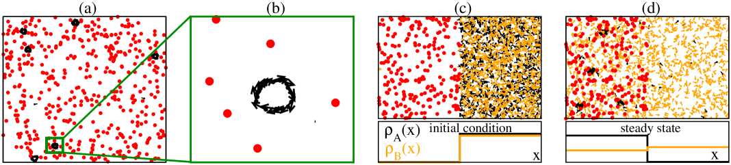
Figure 2: Trapping and filtering. For large values of $\gamma$ and $\rho_{o}$, spontaneous trapping of particle occurs, see (a) where $\gamma=5$, $\rho_{o}=0.5$, $\eta=0.01$, and $L=30$. Obstacles are indicated by red dots while black arrows correspond to SPPs. Inside traps particles self-organize into vortex-like structures, (b) commentMovies . Spontaneous trapping leads to subdiffusion as indicated in Fig. 3 and can be used to design filters. Starting with an initial condition as in (c), with two types of particles, characterized by $\gamma_{A}=5$ and $\gamma_{B}=1$, we quickly arrive to a steady state where $A$ particles are confined to the left half of the box, while $B$ particles diffusive freely over the system. The lower panels in (c) and (d) indicate the density projected on the x-axis of $A$ and $B$ particles.

By performing a moment expansion of Eq. (4), where we define $\rho(\mathbf{x},t)=\int d\theta p$, $P_{x}(\mathbf{x},t)=\int d\theta\cos(\theta)p$, $P_{y}(\mathbf{x},t)=\int d\theta\sin(\theta)p$, and $Q_{s}(\mathbf{x},t)=\int d\theta\sin(2\theta)p$, and $Q_{c}(\mathbf{x},t)=\int d\theta\cos(2\theta)p$, we arrive to the following set of equations:

$$\partial_{t}\rho = -v_{0}\nabla.\mathbf{P}$$ (6)

$$\partial_{t}P_{x} = -\frac{v_{0}}{2}\nabla.\left[Q_{c}+\rho,Q_{s}\right]-\tilde{\mathcal{D}}_{\theta}P_{x}$$ (7)

$$\partial_{t}P_{y} = -\frac{v_{0}}{2}\nabla.\left[Q_{s},\rho-Q_{c}\right]-\tilde{\mathcal{D}}_{\theta}P_{y}\,,$$ (8)

where we assumed that $\partial_{t}Q_{c}=\partial_{t}Q_{s}=0$. It can be shown that the temporal evolution of $Q_{c}$ and $Q_{s}$ is faster than the one of $P_{x}$ and $P_{y}$, which in turn is faster than the one for $\rho$. Since we are interested in the long time behavior of $\rho(\mathbf{x},t)$, and there is no induced order, we take $Q_{c}=Q_{s}=0$ and use the fast relaxation of Eqs. (7) and (8) to express $P_{x}$ and $P_{y}$ as slave functions of $\rho$ and its derivatives  comment1 . This procedure leads to the following asymptotic equation for $\rho(\mathbf{x},t)$:

$$\partial_{t}\rho = \nabla.\left[\frac{v_{0}^{2}}{2\tilde{\mathcal{D}}_{\theta}}\nabla\rho\right]\,.$$ (9)

From Eq. (9), it is evident that the spatial diffusion coefficient $D_{x}$ takes the form: $D_{x}=v_{0}^{2}/\left[2\left(D_{\theta}+\Lambda_{0}\rho_{o}\right)\right]$, with $\Lambda_{0}=v_{0}\sigma_{0}\epsilon_{\theta}^{2}/6$. Notice that $D_{x}$ is a decreasing function of $\rho_{o}$ comment2 .

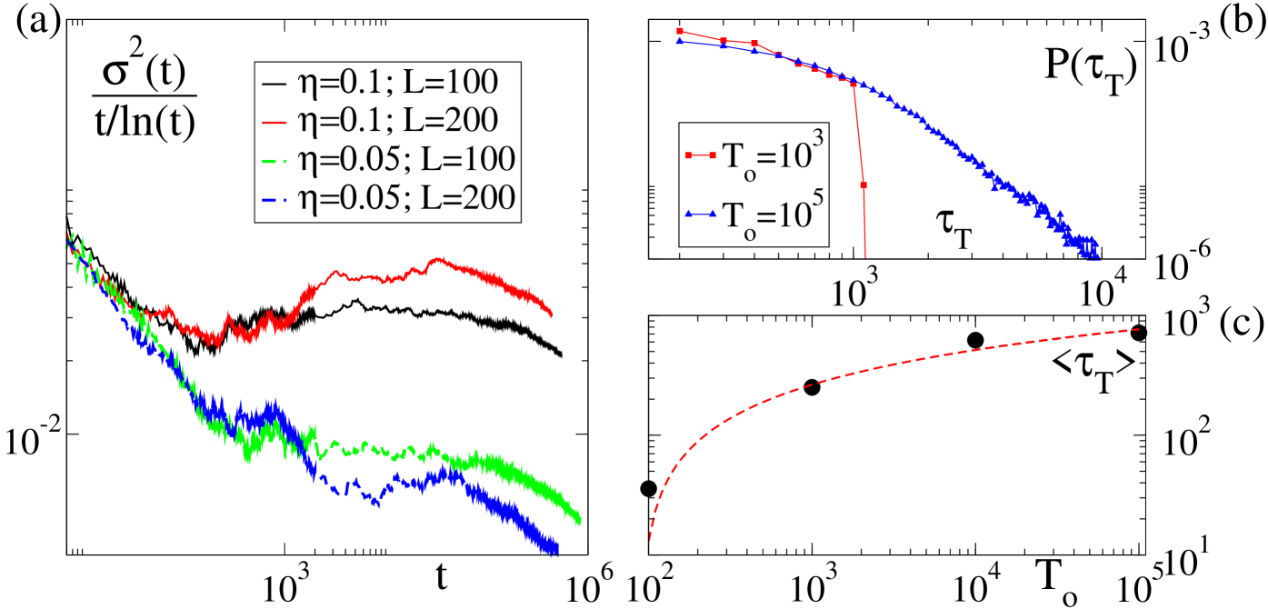
Figure 3: Genuine subdiffusive behavior. (a) scaling of the mean square displacement $\sigma^{2}(t)$ with $t$ for two system sizes, with $N_{p}/L^{2}=1$, $\rho_{o}=0.5$ and $\gamma=5$. Notice that the growth of $\sigma^{2}(t)$ is even slower than $t/\ln(t)$. (b) the distribution of trapping times $P(\tau_{T})$ is power-law distributed for long enough $T_{o}$. (c) the average waiting time $\langle\tau_{T}\rangle$ is an increasing function of $T_{o}$. The red dashed curve corresponds to a fit $\propto\ln(T_{o})$. Measurements in (b) and (c) were performed on a particular trap for $\eta=0.1$.

High-density approximation.– At large obstacle densities, particles always sense the presence of several obstacles around them. This means that we cannot think of collisions as rare sudden jumps in the moving direction. Thus, we replace Eq. (5) with a direct, local, coarse-grained expression for the interactions. This means that we leave the Boltzmann-like for the Fokker-Planck approach where the interaction with obstacles is expressed by $F=\partial_{\theta}\left[Ip(\mathbf{x},\theta,t)\right]$. The term $I$ represents the (average) interaction felt by a particle at $\mathbf{x}$ moving in direction $\theta$, which takes the form:

$$I=\frac{\gamma}{n(\mathbf{x})}\sum_{j}\sin(\theta-\alpha_{j})=\frac{\gamma\Gamma(\mathbf{x})}{n(\mathbf{x})}\sin(\theta-\psi(\mathbf{x}))\,,$$ (10)

where $j$ is an index that runs over all neighboring obstacles, $\alpha_{j}$ is the polar angle associated to the vector $\mathbf{x}-\mathbf{y}_{j}$, and $\Gamma(\mathbf{x})$ and $\psi(\mathbf{x})$ are the modulus and phase, respectively, of $\sum_{j}\exp(\imath(\alpha_{j}))$, see kuramoto1975 . We now approximate Eq. (10) by its average and use the fact that it represents a sum of $n$ random vectors of magnitude $1$ in the complex plane, to express $I\sim\sin(\theta-\psi(\mathbf{x}))/\sqrt{n}$, where $n\approx\pi R^{2}\rho_{o}$. Inserting this approximated expression into Eq. (4) and performing the moment expansion and approximations that led us from Eqs. (6)-(8) to Eq. (9), we arrive to:

$$\partial_{t}\rho = \frac{v_{0}^{2}}{2D_{\theta}}\nabla^{2}\rho-\frac{\gamma v_{0}}{2D_{\theta}R\sqrt{\pi\rho_{0}}}\nabla.\left[(\cos(\psi),\sin(\psi))\rho\right]$$ (11)

$$= \frac{v_{0}^{2}}{2D_{\theta}}\nabla^{2}\rho-\frac{\gamma v_{0}}{2D_{\theta}R\sqrt{\pi\rho_{0}}}\nabla.\left[\frac{\rho\nabla\rho_{o}(\mathbf{x})}{||\nabla\rho_{o}(\mathbf{x})||}\right]\,,$$

where we have approximated the vector field $(\cos(\psi),\sin(\psi))\sim\nabla\rho_{o}(\mathbf{x})/||\nabla\rho_{o}(\mathbf{x})||$. If we replace our current definition of $\rho$ by a local average over a volume of linear dimensions much larger than $R$ and look for the long-time dynamics of this redefined density, by applying homogenization techniques, we expect to recover a diffusive behavior with a new effective diffusion, whose explicit form depends on the statistical properties of the random field $\rho_{o}(\mathbf{x})$ and is proportional to the square of the constant in front of the convective term. While according to Eq. (9) (LD approx.), $D_{x}\to 0$ as $\rho_{o}\to\infty$, Eq. (11) (i.e., the HD approx.) indicates that in the limit of $\rho_{o}\to\infty$, $D_{x}\to D_{x0}$, where $D_{x0}$ is the diffusion coefficient in absence of obstacles defined above. These two results necessarily imply the existence of a minimum in the spatial diffusion coefficient $D_{x}$ as $\rho_{o}$ is increased from $0$ to $\infty$. Moreover, this minimum has to be located at the crossover between the LD and HD approximation, which can be roughly estimated to occur at $\rho_{c}\sim 1/(\pi R^{2})$, around which, $D_{x}\sim 1/\left[\rho_{c}-\Lambda_{1}\rho_{o}\right]$, with $\Lambda_{1}$ a constant. All these findings are confirmed by particle simulations as shown in Fig. (1).

Trapping.– Eq. (11) indicates that the vector field $\nabla\rho_{o}(\mathbf{x})$ governs the long-term dynamics at high obstacle concentrations. In particular, the random distribution of obstacles, together with the compressible nature of $\rho(\mathbf{x},t)$, may result in the spontaneous formation of active particle sinks. These topological defects, which we refer to as “traps”, are indeed observed in simulations for large values of $\gamma$, Fig. 2(a) and (b). Inside traps particles form vortex-like patterns. The average time $\langle\tau_{T}\rangle$ spent by a particle inside a trap depends on the precise configuration of the obstacles that form the trap. We find that the presence of traps can lead to a genuine subdiffusive behavior, with particles exhibiting a mean-square displacement $\sigma^{2}(t)=\langle\mathbf{x}^{2}(t)\rangle$ that grows slower than $t$. To test this observation, let us assume that particle motion can be conceived as a random walk across a two dimensional array of traps such that $\sigma^{2}(t)\propto n_{J}(t)$ where $n_{J}(t)$ represents the number of jumps from trap to trap the random walker performs during $t$. To estimate $n_{J}(t)$, we study the distribution to trapping times $P(\tau_{T})$ of a given trap, see Fig. 3(b). Subdiffusion can only occur if $P(\tau_{T})$ is asymptotically power-law distributed and such that $\langle\tau_{T}\rangle$ grows with the observation time $T_{o}$ as $\ln(T_{o})$ or faster Krapivsky et al. (2010), see Fig. 3(b) and (c). Within this simplified picture, the behavior of $\langle\tau_{T}\rangle$ shown in Figs. 3(c) suggests that $\sigma^{2}(t)\propto n_{J}(t)\sim t/\ln(t)$. By taking $t\to\infty$, we expect $\sigma^{2}(t)/[t/\ln(t)]$ to approach a constant value. Fig. 3(a) clearly shows that $\sigma^{2}(t)$ is slower than $t/\ln(t)$. Arguably, this is due to the fact that once a particle escapes from a trap, typically it performs a small excursion before being reabsorbed by the same trap.

Discussion.– The spontaneous trapping of particles depends not only on $\rho_{o}$ but also on $\gamma$, which is an intrinsic property of the particle. This means that given the same spatial environment, two particle types, say characterized by $\gamma_{A}$ and $\gamma_{B}$, will respond differently. We can make use of this fact to fabricate a simple and cheap filter as indicated in Fig. 2(c) and (d). Notice that trapping of one of the particle types is required to obtain this effect. A different diffusion coefficient for $A$ and $B$ particles on the left half of the box does not suffice to induce higher concentration of one particle type to the left.

Trapping, rectification, and sorting have been reported for a particular kind of active particles: chiral, i.e. circularly moving particles mijalkov2013 ; reichhardt2013 . By placing L-shaped obstacles on a regular lattice, the motion of such particles can be rectified reichhardt2013 , while elongated obstacles arranged in flower-like patterns can be used to selectively trap either levogyre or dextrogyre particles mijalkov2013 . For non-chiral active particle, trapping and rectification can be achieved by using V-shape objects. Kaiser et al. in kaiser2012 ; kaiser2013 showed that self-propelled rods can be trapped by placing V-shape objects. These traps provide a geometrical constrain to the active particles that end up being blocked in the V-shape devices. On the other hand, by arranging in line V-shape objects, but with their tips open, rectification of particle motion can be achieved galajda2007 ; Tailleur and Cates (2009). These V-shape objects, either with their tip closed or opened, cannot be used to produce a filter of active particles. Closed V-shape objects collect, by imposing geometric obstruction, any kind of self-propelled particle, while in opened V-shape objects clogging of large size particles necessary occurs, preventing particle flow. Notice that the novel trapping and sorting mechanism reported here, which is based on the obstacle avoidance response time, is generic and should apply to all kind of active particles, including interacting, non-interacting, chiral or non-chiral active particles.

Finally, it is important to mention that genuine subdiffusion occurs for fixed obstacles only. For slowly diffusing obstacles, i.e. for a (slow) dynamic environment, the asymptotic behavior of the active particles is diffusive. The low and high density approximations, given by Eq. (9) and (11), provide a reasonable description of particle motion even for dynamical environments as long as obstacle diffusion remains substantially smaller than the active motion. Furthermore, trapping and subdiffusive behavior is also observed for interacting active particles as those studied in chepizhko2013 for values of the interaction strength significantly smaller than those associated to obstacle avoidance commentMovies .

Numerical simulations have been performed at the ‘Mesocentre SIGAMM’ machine, hosted by Observatoire de la Côte d’Azur. We thank F. Delarue and R. Soto for valuable comments on the manuscript and the Fed. Doeblin for partial financial support.

References

- Berg (1983) H. Berg, Random walks in biology (Princeton University Press, Princeton, 1983).
- Okubo and Levin (1980) A. Okubo and S. Levin, Diffusion and ecological problems (Springer, New York, 1980).
- Metzler and Klafter (2000) R. Metzler and J. Klafter, Physics Reports 339, 1 (2000).
- (4) P. Romanczuk et al., Eur. Phys. J. Special Topics 202, 1 (2012).
- Vicsek and Zafeiris (2012) T. Vicsek and A. Zafeiris, Physics Reports 517, 71 (2012).
- Ramaswamy (2010) S. Ramaswamy, Annual Review of Condensed Matter Physics 1, 323 (2010).
- (7) F. Peruani et al., Phys. Rev. Lett. 108, 098102 (2012).
- (8) F. Ginelli et al., Phys. Rev. Lett. 104, 184502 (2010).
- Peruani and Morelli (2007) F. Peruani and L. Morelli, Phys. Rev. Lett. 99, 010602 (2007).
- Golestanian (2009) R. Golestanian, Phys. Rev. Lett. 102, 188305 (2009).
- Romanczuk and Schimansky-Geier (2011) P. Romanczuk and L. Schimansky-Geier, Phys. Rev. Lett. 106, 230601 (2011).
- (12) P. Galajda et al., J. Bacterial. 189, 8704 (2007).
- Wensink and Löwen (2008) H. H. Wensink and H. Löwen, Phys. Rev. E 78, 031409 (2008).
- (14) M. Wand et al., Phys. Rev. Lett. 101, 018102 (2008).
- Tailleur and Cates (2009) J. Tailleur and M. Cates, Europhys. Lett. 86, 60002 (2009).
- Radtke and Schimansky-Geier (2012) P. Radtke and L. Schimansky-Geier, Phys. Rev. E 85, 051110 (2012).
- (17) Kudrolli et al., Phys. Rev. Lett. 100, 058001 (2008).
- Kudrolli et al. (2006) A. Kudrolli, G. Lumay, D. Volfson, and L. Tsimring, Phys. Rev. E 74, 030904(R) (2006).
- Deseigne et al. (2010) J. Deseigne, O. Dauchot, and H. Chaté, Phys. Rev. Lett. 105, 098001 (2010).
- (20) C. A. Weber et al., Phys. Rev. Lett. 110, 208001 (2013).
- Jiang et al. (2010) H.-R. Jiang, N. Yoshinaga, and M. Sano, Phys. Rev. Lett. 105, 268302 (2010).
- Golestanian (2012) R. Golestanian, Phys. Rev. Lett. 108, 038303 (2012).
- (23) I. Theurkauff et al., Phys. Rev. Lett. 108, 268303 (2012).
- (24) J. Palacci et al., Science 339, 936 (2013).
- et al. (2004) W. Paxton et al., J. Am. Chem. Soc. 126, 13424 (2004).
- Mano and Heller (2005) N. Mano and A. Heller, J. Am. Chem. Soc. 127, 11574 (2005).
- Rückner and Kapral (2007) G. Rückner and R. Kapral, Phys. Rev. Lett. 98, 150603 (2007).
- (28) J. Howse et al., Phys. Rev. Lett. 99, 048102 (2007).
- R. Golestanian and Ajdari (2005) R. Golestanian, T.B. Liverpool and A. Ajdari, Phys. Rev. Lett. 94, 220801 (2005).
- (30) B. Alberts et al, Molecular biology of the cell (Garland publishing, 1994).
- Dworkin (1993) M. Dworkin, Myxobacteria II (Amer Society for Microbiology, 1993).
- Bouchaud and Geoges (1990) J.-P. Bouchaud and A. Geoges, Physics Reports 195, 127 (1990).
- Berry and Chaté (2011) H. Berry and H. Chaté, arXiv:1103.2206 (2011).
- (34) The boundary has been numerically estimated by: i) Studying – for subdiffusive particles never saturates. ii) By measuring the asymptotic fraction of particle on the left half of the box in systems prepared as indicated in Fig. 2(c) and (d) – values of this quantity above can only occur due to the presence of traps. Both methods, i) and ii), led to the same boundary estimate.
- (35) Collective effects of an interacting version of this model were studied in chepizhko2013 . Here, we focus on individual locomotion patterns.
- (36) O. Chepizhko, E.G. Altmann, and F. Peruani, Phys. Rev. Lett. 110, 238101 (2013).
- (37) C. W. Gardiner, Handbook of Stochastic Methods (Springer, Heildelberg, 2004).
- (38) We reserve the symbol , without dependency, to the global obstacle density.
- (39) Alternatively, multi-scaling analysis can be used to go from Eqs. (4) and (5) to Eq. (9).
- (40) There are qualitative differences with the Lorentz gas model, see Krapivsky et al. (2010). Firstly, in our model angular diffusion acts on the moving particles in between collisions. Secondly, the scattering process is not an instantaneous process and leads, given the absence of conserved quantities, to a non bijective relationship between the impact parameter and the scattered angle.
- (41) Y. Kuramoto, in International Problems in Theoretical Physics, edited by H. Araki, Lecture Notes in Physics (Springer, New York, 1975).
- (42) See supplemental material at XXXX for movies.
- Krapivsky et al. (2010) P. L. Krapivsky, S. Redner, and E. Ben-Naim, A kinetic view of statistical physics (Cambridge University Press, New York, 2010).
- (44) M. Mijalkov and G. Volpe, Soft Matter 9, 6376 (2013).
- (45) C. Reichhardt, C.J. Olson Reichhardt, arXiv:1307.0755 (2013).
- (46) A. Kaiser et al., Phys. Rev. Lett. 108, 268307 (2012).
- (47) A. Kaiser, K. Popowa, H.H. Wensink and H. Löwen, Phys. Rev. E 88, 022311 (2013).