The Fermi-LAT Collaboration
Dark Matter Constraints from Observations of 25 Milky Way Satellite Galaxies with the Fermi Large Area Telescope
Abstract
The dwarf spheroidal satellite galaxies of the Milky Way are some of the most dark-matter-dominated objects known. Due to their proximity, high dark matter content, and lack of astrophysical backgrounds, dwarf spheroidal galaxies are widely considered to be among the most promising targets for the indirect detection of dark matter via rays. Here we report on -ray observations of 25 Milky Way dwarf spheroidal satellite galaxies based on 4 years of Fermi Large Area Telescope (LAT) data. None of the dwarf galaxies are significantly detected in rays, and we present -ray flux upper limits between 500 and 500. We determine the dark matter content of 18 dwarf spheroidal galaxies from stellar kinematic data and combine LAT observations of 15 dwarf galaxies to constrain the dark matter annihilation cross section. We set some of the tightest constraints to date on the annihilation of dark matter particles with masses between 2 and 10 into prototypical standard model channels. We find these results to be robust against systematic uncertainties in the LAT instrument performance, diffuse -ray background modeling, and assumed dark matter density profile.
pacs:
95.35.+d, 95.85.Pw, 98.52.WzI Introduction
Astrophysical evidence and theoretical arguments suggest that non-baryonic cold dark matter constitutes of the contemporary Universe (Ade et al., 2013). While very little is known about dark matter beyond its gravitational influence, a popular candidate is a weakly interacting massive particle (WIMP) (Jungman et al., 1996; Bergstrom, 2000; Bertone et al., 2005). From an initial equilibrium state in the hot, dense early Universe, WIMPs can freeze out with a relic abundance sufficient to constitute much, if not all, of the dark matter. Such WIMPs are expected to have a mass in the to range and a -wave annihilation cross section usually quoted at (though, as pointed out by Steigman et al. (2012), a more accurate calculation yields at masses and at higher masses). In regions of high dark matter density, WIMPs may continue to annihilate into standard model particles through processes similar to those that set their relic abundance.
Gamma rays produced from WIMP annihilation, either mono-energetically (from direct annihilation) or with a continuum of energies (through annihilation into intermediate states) may be detectable by the Large Area Telescope (LAT) on board the Fermi Gamma-ray Space Telescope (Fermi) (Atwood et al., 2009). These rays would be produced preferentially in regions of high dark matter density. The LAT has enabled deep searches for dark matter annihilation in the Galactic halo through the study of both continuum and mono-energetic -ray emission (Hooper and Linden, 2011; Ackermann et al., 2012a; Abazajian and Kaplinghat, 2012; Abdo et al., 2010a; Ackermann et al., 2012b; Weniger, 2012; Ackermann et al., 2013a). Additionally, robust constraints have been derived from the isotropic -ray background (Abdo et al., 2010b; Abazajian et al., 2010), galaxy clusters (Ackermann et al., 2010), Galactic dark matter substructures (Zechlin et al., 2012; Ackermann et al., 2012c; Zechlin and Horns, 2012), and the study of nearby dwarf spheroidal galaxies (Abdo et al., 2010c; Ackermann et al., 2011; Geringer-Sameth and Koushiappas, 2011; Mazziotta et al., 2012; Geringer-Sameth and Koushiappas, 2012).
The dwarf spheroidal satellite galaxies of the Milky Way are especially promising targets for the indirect detection of dark matter annihilation due to their large dark matter content, low diffuse Galactic -ray foregrounds, and lack of conventional astrophysical -ray production mechanisms (Mateo, 1998; Grcevich and Putman, 2009). An early analysis by Abdo et al. (2010c) set constraints on the dark matter annihilation cross section from 11-month LAT observations of 8 individual dwarf spheroidal galaxies. In a subsequent effort, Ackermann et al. (2011) presented an improved analysis using 2 years of LAT data, 10 dwarf spheroidal galaxies, and an expanded statistical framework. The analysis of Ackermann et al. (2011) has two significant advantages over previous analyses. First, statistical uncertainties in the dark matter content of dwarf galaxies are incorporated as nuisance parameters when fitting for the dark matter annihilation cross section. Second, observations of the 10 dwarf galaxies are combined into a single joint likelihood analysis for improved sensitivity. The analysis of Ackermann et al. (2011) probes the canonical thermal relic cross section for dark matter masses annihilating through the and channels, while similar studies by Geringer-Sameth and Koushiappas (2011) and Mazziotta et al. (2012) yield comparable results.
The present analysis expands and improves upon the analysis of Ackermann et al. (2011). Specifically, we use a 4-year -ray data sample with an extended energy range from 500 to 500 and improved instrumental calibrations. We constrain the -ray flux from all 25 known Milky Way dwarf spheroidal satellite galaxies in a manner that is nearly independent of the assumed -ray signal spectrum (Section III). We use a novel technique to determine the dark matter content of 18 dwarf spheroidal galaxies by deriving prior probabilities for the dark matter distribution from the population of Local Group dwarf galaxies (Section IV). This allows us to increase the number of spatially-independent dwarf galaxies in the joint likelihood analysis to 15 (Section V). We develop a more advanced statistical framework to examine the expected sensitivity of our search. Additionally, we model the spatial -ray intensity profiles of the dwarf galaxies in a manner that is consistent with their derived dark matter distributions. We perform an extensive study of systematic effects arising from uncertainties in the instrument performance, diffuse background modeling, and dark matter distribution (Section VI). As a final check, we perform a Bayesian analysis that builds on the work of Mazziotta et al. (2012) and yields comparable results (Section VII). No significant -ray emission is found to be coincident with any of the 25 dwarf spheroidal galaxies. Our combined analysis of 15 dwarf spheroidal galaxies yields no significant detection of dark matter annihilation for particles in the mass range from 2 to 10 annihilating to , , , , , or (when kinematically allowed), and we set robust upper limits on the dark matter annihilation cross section.
II Data Selection and Preparation
Since the start of science operations in August of 2008, the LAT has continuously scanned the -ray sky in the energy range from to (Atwood et al., 2009). The LAT has unprecedented angular resolution and sensitivity in this energy range, making it an excellent instrument for the discovery of new -ray sources (Nolan et al., 2012). We select a data sample corresponding to events collected during the first four years of LAT operation (2008-08-04 to 2012-08-04). We use the P7REP data set, which utilizes the Pass-7 event reconstruction and classification scheme (Ackermann et al., 2012d), but was reprocessed with improved calibrations for the light yield and asymmetry in the calorimeter crystals (Bregeon et al., 2013). The new calorimeter calibrations improve the in-flight point-spread function (PSF) above and correct for the small ( per year), expected degradation in the light yield of the calorimeter crystals measured in flight data. Consequently, the absolute energy scale has shifted upward by a few percent in an energy- and time-dependent manner. In addition, the re-calibration of the calorimeter light asymmetry leads to a statistical re-shuffling of the events classified as photons.
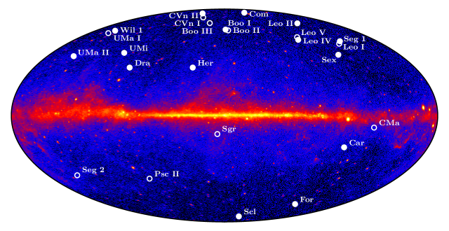
We select events from the P7REP CLEAN class in the energy range from to and within a 10∘ radius of 25 dwarf spheroidal satellite galaxies (Figure 1). The CLEAN event class was chosen to minimize particle backgrounds while preserving effective area. At high Galactic latitudes in the energy range from to , the particle background contamination in the CLEAN class is of the extragalactic diffuse -ray background (Ackermann et al., 2012d), while between and the particle background is comparable to systematic uncertainties in the diffuse Galactic -ray emission. Studies of the extragalactic -ray background at energies greater than suggest that at these energies the fractional residual particle background is greater than at lower energies Ackermann et al. (2013b). To reduce -ray contamination from the bright limb of the Earth, we reject events with zenith angles larger than 100∘ and events collected during time periods when the magnitude of rocking angle of the LAT was greater than 52∘.
We create regions-of-interest (ROIs) by binning the LAT data surrounding each of the 25 dwarf galaxies into 0.1∘ pixels and into 24 logarithmically-spaced bins of energy from to . We model the diffuse background with a structured Galactic -ray emission model (gll_iem_v05.fit) and an isotropic contribution from extragalactic rays and charged particle contamination (iso_clean_v05.txt).111http://fermi.gsfc.nasa.gov/ssc/data/access/lat/BackgroundModels.html We build a model of point-like -ray background sources within 15∘ of each dwarf galaxy beginning with the second LAT source catalog (2FGL) (Nolan et al., 2012). We then follow a procedure similar to that of the 2FGL to find additional candidate point-like background sources by creating a residual test statistic map with pointlike (Nolan et al., 2012). No new sources are found within 1∘ of any dwarf galaxy and the additional candidate sources have a negligible impact on our dwarf galaxy search. We use the P7REP_CLEAN_V15 instrument response functions (IRFs) corresponding to the LAT data set selected above. When performing the Bayesian analysis in Section VII, we utilize the same LAT data set but follow different data preparation and background modeling procedures, which are described in that section.
III Maximum Likelihood Analysis
Limited -ray statistics and the strong dependence of the LAT performance on event energy and incident direction motivate the use of a maximum likelihood-based analysis to optimize the sensitivity to faint -ray sources. We define the standard LAT binned Poisson likelihood,
| (1) |
as a function of the photon data, , a set of signal parameters, , and a set of nuisance parameters, . The number of observed counts in each energy and spatial bin, indexed by , depends on the data, , while the model-predicted counts depend on the input parameters, . This likelihood function encapsulates information about the observed counts, instrument performance, exposure, and background fluxes. However, this likelihood function is formed “globally” (i.e., by tying source spectra across all energy bins simultaneously) and is thus necessarily dependent on the spectral model assumed for the source of interest. To mitigate this spectral dependence, it is common to independently fit a spectral model in each energy bin, (i.e., to create a spectral energy distribution for a source) Abdo et al. (2010d). This expands the global parameters and into sets of independent parameters and . Likewise, the likelihood function in Equation (1) can be reformulated as a “bin-by-bin” likelihood function,
| (2) |
In Equation (2) the terms in the product are independent binned Poisson likelihood functions, akin to Equation (1) but with the index only running over spatial bins.
By analyzing each energy bin separately, we remove the requirement of selecting a global spectrum to span the entire energy range at the expense of introducing additional parameters into the fit. If the source of interest is bright, it is possible to profile over the spectral parameters of the background sources as nuisance parameters in each energy bin. However, for faint or undetected sources it is necessary to devise a slightly modified likelihood scheme where the nuisance parameters in all energy bins are set by the global maximum likelihood estimate,222For brevity we assume that all nuisance parameters are globally fit, but it is straightforward to generalize to the situation where some nuisance parameters are defined independently in each bin.
| (3) |
Fixing the normalizations of the background sources at their globally fit values avoids numerical instabilities resulting from the fine binning in energy and the degeneracy of the diffuse background components at high latitude. Thus, for the analysis of dwarf galaxies our bin-by-bin likelihood becomes
| (4) |
The bin-by-bin likelihood is powerful because it makes no assumption about the global signal spectrum.333The second order spectral dependence arising from the choice of a spectral model within each bin is found to be for our energy bin size. However, it is easy to recreate a global likelihood function to test a given signal spectrum by tying the signal parameters across the energy bins,
| (5) |
As a consequence, computing a single bin-by-bin likelihood function allows us to subsequently test many spectral models rapidly. In practice, the signal parameters derived from the global likelihood function in Equation (5) are found to be equivalent to those derived from Equation (1) so long as couplings between the signal and nuisance parameters are small.
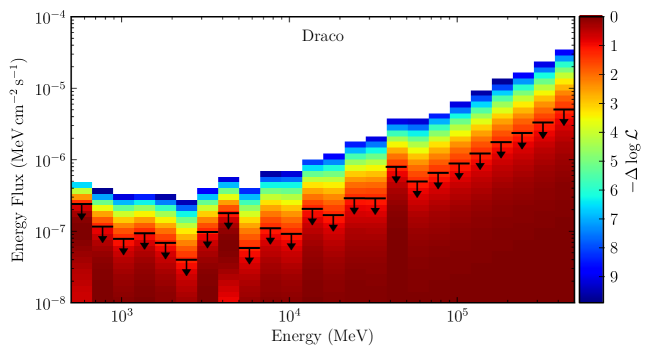
For each of the 25 dwarf galaxies listed in Table 1, we construct a bin-by-bin likelihood function. Normalizations of the background sources (both point-like and diffuse) are fixed from a global fit over all energy bins.444Including the putative dwarf galaxy source in the global fit has a negligible () impact on the fitted background normalizations. The signal spectrum within each bin is modeled by a power law (), and the signal normalization is allowed to vary independently between bins. In each bin, we set a 95% confidence level (CL) upper limit on the energy flux from the putative signal source by fixing the parameters of all other bins and finding the value of the energy flux where the log-likelihood has decreased by from its maximum (the “delta-log-likelihood technique”) Bartlett (1953); Rolke et al. (2005). Figure 2 illustrates the detailed bin-by-bin LAT likelihood result for the Draco dwarf spheroidal galaxy.
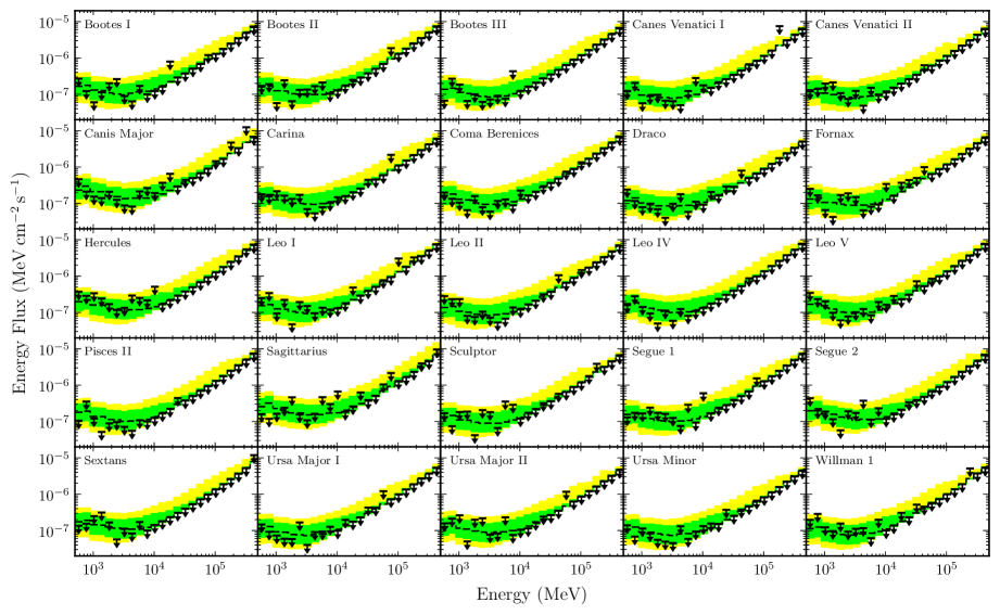
In Figure 3, we compare the observed bin-by-bin flux upper limits for all 25 dwarf spheroidal galaxies to those derived for 2000 realistic background-only simulations. These simulations are generated with the LAT simulation tool gtobssim using the in-flight pointing history and instrument response of the LAT and including both diffuse and point-like background sources. We find that the observed limits are consistent with simulations of the null hypothesis. We emphasize that these bin-by-bin limits are useful because they make no assumptions about the annihilation channel or mass of the dark matter particle.
While the bin-by-bin likelihood function is essentially independent of spectral assumptions, it does depend on the spatial model of the target source. The dark matter distributions of some dwarf galaxies may be spatially resolvable by the LAT (Charbonnier et al., 2011). Thus, for dwarf galaxies for which stellar kinematic data sets exist, we model the -ray intensity from the line-of-sight integral through the best-fit dark matter distribution as derived in Section IV.2. Dwarf galaxies that lack stellar kinematic data sets are modeled as point-like -ray sources. Possible systematic uncertainty associated with the analytic form and spatial extent of the dark matter profile are discussed in Section IV.2 and Section VI.
IV Dark Matter Annihilation
The integrated -ray signal flux at the LAT, (), expected from dark matter annihilation in a density distribution, , is given by
| (6) |
Here, the term is strictly dependent on the particle physics properties — i.e., the thermally-averaged annihilation cross section, , the particle mass, , and the differential -ray yield per annihilation, , integrated over the experimental energy range.555Strictly speaking, the differential yield per annihilation in Equation (6) is a sum of differential yields into specific final states: , where is the branching fraction into final state . In the following, we make use of Equation (6) in the context of single final states only. The is the line-of-sight integral through the dark matter distribution integrated over a solid angle, . Qualitatively, the encapsulates the spatial distribution of the dark matter signal, while sets its spectral character. Both and the contribute a normalization factor to the signal flux.
IV.1 Particle Physics Factor
We generate -ray spectra for dark matter annihilation with the DMFIT package (Jeltema and Profumo, 2008) as implemented in the LAT ScienceTools. We have upgraded the spectra in DMFIT from Pythia 6.4 (Sjöstrand et al., 2006) to Pythia 8.165 (Sjöstrand et al., 2008). We generate -ray spectra for the and channels from analytic formulae, i.e., Equation (4) in Essig et al. (2009) (see also Beacom et al. (2005); Birkedal et al. (2005)). For the muon channel, we add the contribution from the radiative decay of the muon () using Equations (59), (61), and (63) from Mardon et al. (2009); this can have a factor-of-two effect on the integrated photon yield for . We also extend the range of dark matter masses in DMFIT to lower () and higher () masses (Jeltema and Profumo, 2008). Thus, the upgraded DMFIT includes -ray spectra for dark matter annihilation through 12 standard model channels (, , , , , , , , , , , ) for 24 dark matter masses between 2 and 10 (when kinematically allowed). Annihilation spectra for arbitrary dark matter masses within this range are generated by interpolation. Appropriate flags are set in Pythia to generate spectra for dark matter masses below 10. However, we note that we ignore the effect of hadronic resonances, which could be important for some dark matter models with masses less than . In addition, the hadronization model used in Pythia becomes more uncertain at lower energies. The new spectra are consistent with those calculated in Jeltema and Profumo (2008) for dark matter masses between and . Outside of this range we believe that the new spectra are a more accurate representation of the underlying physics since they are derived by modeling some of the relevant physical processes, rather than by ad hoc extrapolations.
IV.2 J-Factors for Dwarf Spheroidal Galaxies
The dark matter content of dwarf spheroidal galaxies can be determined through dynamical modeling of their stellar density and velocity dispersion profiles (see a recent review by Battaglia et al. (2013)). Recent studies have shown that an accurate estimate of the dynamical mass of a dwarf spheroidal galaxy can be derived from measurements of the average stellar velocity dispersion and half-light radius alone (Walker et al., 2009; Wolf et al., 2010). The total mass within the approximate half-light radius and likewise the integrated have been found to be fairly insensitive to the assumed dark matter density profile (Martinez et al., 2009; Strigari, 2013). We use the prescription of Martinez (2013) to calculate for a subset of 18 Milky Way dwarf spheroidal galaxies possessing dynamical mass estimates constrained by stellar kinematic data sets (Table 1) Dall’Ora et al. (2006); Simon and Geha (2007); Walker et al. (2009); Mateo et al. (2008); Koch et al. (2007); Simon et al. (2011); Muñoz et al. (2005); Willman et al. (2011).
We construct a likelihood function for each individual dwarf spheroidal galaxy from the observed luminosity, half-light radius, , and mass within the half-light radius, , together with their associated uncertainties. We derive priors on the relationships between the luminosity, , maximum circular velocity, , and radius of maximum circular velocity, , from the ensemble of Local Group dwarf galaxies (Strigari et al., 2008a). By implementing this analysis as a two-level Bayesian hierarchical model Loredo and Hendry (2009), we are able to simultaneously constrain both the priors and the resulting likelihoods for the dynamical properties of the dwarf galaxies Martinez (2013). This approach benefits from utilizing all available knowledge of the dark matter distribution in these objects while mitigating any systematic differences between the observed dwarf galaxies and numerical simulations Springel et al. (2008); Diemand et al. (2007).
While priors on the relationships between, , , and can be derived from the data, their form must be chosen a priori. Motivated by simulations Springel et al. (2008); Diemand et al. (2007), we assume a prior on the relationship between and that follows a linear form between and with an intrinsic Gaussian scatter ,
| (7) |
Similarly, we assume that the prior in is linearly related to with Gaussian scatter,
| (8) |
Finally, we assume a power-law prior on the galaxy luminosity function Koposov et al. (2008),
| (9) |
The 7 free parameters of these priors, , are derived from the full Local Group dwarf galaxy sample. Additionally, each dwarf is described by its measured half-light radius, the mass within this radius, the total luminosity, and the associated errors on these quantities. We constrain the full set of parameters with a Metropolis nested sampling algorithm with approximately 500,000 points per chain (Skilling, 2004).
The inner slope of the dark matter density profile in dwarf galaxies remains a topic of debate (Gilmore et al., 2007; Strigari et al., 2010; Walker and Penarrubia, 2011; Agnello and Evans, 2012). Thus, we repeat the above procedure for two different choices of the dark matter profile: (i) a cuspy Navarro-Frenk-White (NFW) profile (Navarro et al., 1997), and (ii) a cored Burkert profile (Burkert, 1995):
| (10) | |||||
| (11) |
After deriving the halo parameters for each form of the dark matter density profile, we perform the line-of-sight integral in Equation (6) to calculate the intensity profile and integrated within an angular radius of 0.5∘ (). Values of the integrated and spatial extension parameter (defined as the angular size of the scale radius) are included in Table 1. We cross check these results with those derived from an analysis using priors derived from numerical simulations Strigari et al. (2008b); Martinez et al. (2009); Ackermann et al. (2011) and flat, “non-informative” priors Strigari et al. (2008a); Charbonnier et al. (2011). We find that the resulting are consistent within their stated uncertainties. We confirm that the integrated within 0.5∘ is fairly insensitive to the choice of dark matter density profile so long as the central value of the slope is less than Strigari et al. (2008b). Thus, we default to modeling the dark matter distributions within the dwarf galaxies with a NFW profile and examine the impact of this choice in more detail in Section VI.
V Constraints on Dark Matter
V.1 Individual Dwarf Galaxies
For each of the 25 dwarf galaxies listed in Table 1, we use Equation (5) to create global likelihood functions for 6 representative dark matter annihilation channels (, , , , , and ) and a range of particle masses from 2 to 10 (when kinematically allowed). We define a test statistic () as the difference in the global log-likelihood between the null () and alternative hypotheses () Mattox et al. (1996); Nolan et al. (2012),
| (12) |
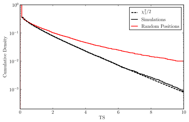
We note that this definition of differs slightly from that commonly used, since the background parameters are fixed at their best-fit values (Section III). We find that the distribution derived from simulations is well matched to a distribution with one bounded degree of freedom, as predicted by the asymptotic theorem of Chernoff (1954) (Figure 4). However, the study of random high-latitude blank fields suggests that the significance calculated from asymptotic theorems is an overestimate of the true signal significance (Section VI). We find no significant -ray excess coincident with any of the 25 dwarf galaxies for any annihilation channel or mass.666We note that are not required to test the consistency of the -ray data with spectral models of dark matter annihilation.
The largest deviation from the null hypothesis, , occurs when fitting the Sagittarius dwarf spheroidal galaxy. Sagittarius is located in a region of intense Galactic foreground emission and is coincident with proposed jet-like structures associated with the Fermi Bubbles (Su et al., 2010; Su and Finkbeiner, 2012). We thus find that systematic changes to the model of the diffuse -ray emission (Section VI) can lead to changes of in this region.
To derive constraints on the dark matter annihilation cross section, we utilize the kinematically determined derived in Section IV.2. We select a subset of 18 dwarf galaxies, excluding the 7 galaxies that lack kinematically determined : Bootes II, Bootes III, Canis Major, Leo V, Pisces II, Sagittarius,777While some authors have suggested a large dark matter component in the Sagittarius dwarf (Aharonian et al., 2008), tidal stripping of this system leads to complicated stellar kinematics (Frinchaboy et al., 2012). and Segue 2. Statistical uncertainty in the determination is incorporated as a nuisance parameter in the maximum likelihood formulation. Thus, the likelihood function for each dwarf galaxy, , is described by,
| (13) | ||||
Here, denotes the individual LAT likelihood function for a single ROI from Equation (5) and the include both the flux normalizations of background -ray sources (diffuse and point-like) and the associated dwarf galaxy J-factors and statistical uncertainties. We fix the background normalizations at their best-fit values and profile over the uncertainties as nuisance parameters to construct a 1-dimensional likelihood function for the dark matter annihilation cross section (Rolke et al., 2005). We note here that the uncertainties must be incorporated as nuisance parameters at the level of the global maximum likelihood fit and not on a bin-by-bin basis. Applying uncertainties to each energy bin individually would multi-count these uncertainties when creating the global likelihood function.
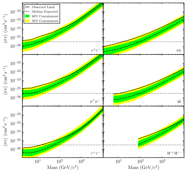
For each of the 18 dwarf galaxies with kinematically determined , we create global likelihood functions incorporating uncertainties on the and derive 95% CL upper limits on the dark matter annihilation cross section using the delta-log-likelihood technique (Tables 2-7). From simulations of the regions surrounding each dwarf galaxy, we confirm the well-documented coverage behavior of this technique, finding that the limit often tends to be somewhat conservative (Rolke et al., 2005). As can be seen from Tables 4-6, the results for several individual dwarf galaxies (i.e., Draco, Coma Berenices, Ursa Major II, Segue 1, and Ursa Minor) probe the canonical thermal relic cross section of for low dark matter masses.
V.2 Combined Analysis
Under the assumption that the characteristics of the dark matter particle are shared across the dwarf galaxies, the sensitivity to weak signals can be increased through a combined analysis. We create a joint likelihood function from the product of the individual likelihood functions for each dwarf galaxy,
| (14) |
The joint likelihood function ties the dark matter particle characteristics (i.e., cross section, mass, branching ratio, and thus -ray spectrum) across the individual dwarf galaxies. From the starting set of 18 dwarf galaxies with kinematically determined , we select a set of non-overlapping dwarfs to ensure statistical independence between observations. When the ROIs of multiple dwarf galaxies overlap, we retain only the dwarf galaxy with the largest . This selection excludes 3 dwarf galaxies: Canes Venatici I in favor of Canes Venatici II, Leo I in favor of Segue 1, and Ursa Major I in favor of Willman 1. Thus, we are left with a subset of 15 dwarf spheroidal galaxies as input to the joint likelihood analysis: Bootes I, Canes Venatici II, Carina, Coma Berenices, Draco, Fornax, Hercules, Leo II, Leo IV, Sculptor, Segue 1, Sextans, Ursa Major II, Ursa Minor, and Willman 1.
No significant signal is found for any of the spectra tested in the combined analysis, prompting us to calculate 95% CL constraints on using the delta-log-likelihood procedure described above (Figure 5). We repeat the combined analysis on a set of random high-latitude blank fields in the LAT data to calculate the expected sensitivity (Section VI). When calculating the expected sensitivity, we randomize the nominal in accord with their measurement uncertainties to form an unconditional ensemble Demortier (2003); Gross (2011). Thus, we note that the positions and widths of the expected sensitivity bands in Figure 5 reflect the range of statistical fluctuations expected both from the LAT data and from the stellar kinematics of the dwarf galaxies. The largest deviation from the null hypothesis occurs for dark matter masses between 10 and 25 annihilating through the channel and has . The conventional threshold for LAT source discovery is Nolan et al. (2012). Studies of random blank-sky locations (Section VI) show that this cannot be naively converted to a significance using asymptotic theorems. Thus, we derive a global p-value directly from random blank high-Galactic-latitude sky positions yielding . This global p-value includes the correlated trials factor resulting from testing dark matter spectral models. As noted by Hooper and Linden (2011), it is difficult to distinguish the -ray spectra of a dark matter particle annihilating into and a lower-mass dark matter particle () annihilating to . However, the quoted above for the channel is larger than that found for any of the masses scanned in the channel. Our analysis agrees well with a standard global LAT ScienceTools analysis using the MINUIT subroutine MINOS (James and Roos, 1975).
The sensitivity of the combined analysis depends most heavily on the observations of the dwarf galaxies with the largest . Specifically, the results of the combined analysis are dominated by Coma Berenices, Draco, Segue 1, Ursa Major II, Ursa Minor, and Willman 1. Because the combined analysis is dominated by a few dwarf galaxies with high , any statistical fluctuation in the combined results will necessarily be associated to an excess coincident with these dwarf galaxies. We find that the primary contributors to the deviation of the combined analysis from the null hypothesis are the ultra-faint dwarf galaxies Segue 1, Ursa Major II, and Willman 1. We find a comparable -ray excess coincident with Hercules and slightly smaller excesses coincident with Sculptor and Canes Venatici II; however, the relatively small of these dwarf galaxies limit their contribution to the combined analysis. On the other hand, the lack of any -ray excess coincident with Coma Berenices, Draco, or Ursa Minor decreases the significance of the deviation in the combined analysis. Thus, we find no significant correlation between the and the -ray of individual dwarf galaxies. We investigate the impact of removing the ultra-faint dwarf galaxies from the combined analysis at the end of Section VI.888 The results discussed in Section V, including bin-by-bin likelihood functions, are available in a machine-readable format at: http://www-glast.stanford.edu/pub_data/713/.
VI Systematic Studies
In this section we briefly summarize the process for determining the impact of systematic uncertainties in the LAT instrument performance, the diffuse interstellar -ray emission model, and the assumed dark matter density profile of the dwarf spheroidal galaxies. A quantitative summary of these results can be found in Table 8. Additionally, we discuss the analysis of random blank-sky locations to validate the sensitivity and significance as quoted in Section V. Finally, we consider the impact of removing three ultra-faint dwarf galaxies from the combined analysis.
We follow the “bracketing IRF” prescription of Ackermann et al. (2012d) to quantify the impact of uncertainties on the instrument performance. We re-analyze the LAT data using two sets of IRFs: one meant to maximize the sensitivity of the LAT to weak -ray sources, and the other meant to minimize it, consistent with the uncertainties of the IRFs. When creating these bracketing IRFs, we utilize constraints on the systematic uncertainty from Ackermann et al. (2012d): 10% uncertainty on the effective area, 15% uncertainty on the PSF, and a 5% uncertainty on the energy dispersion. The maximized IRFs increase the effective area, decrease the PSF width, and disregard the instrumental energy dispersion. Conversely, the minimized IRFs decrease the effective area, increase the PSF width, and include the instrumental energy dispersion. For each IRF set we re-run the full LAT data analysis to fit the normalizations of all background sources. The resulting impact on the combined limits for the dark matter annihilation cross section are shown in Table 8. Additionally, it should be noted that discrepancies between the IRFs (derived from Monte Carlo simulations) and the true instrument performance could introduce spectral features at the level. Because the putative dark matter spectra are more sharply peaked than the diffuse background components, spectral features induced by the IRFs could masquerade as small positive signals. The impact of these effects is not large enough to introduce a globally significant signal, but may be partially responsible for the observed discrepancy between simulations and LAT data.
To quantify the impact of uncertainties on the interstellar emission modeling, we create a set of 8 alternative diffuse models de Palma et al. (2013). Following the prescription of Ackermann et al. (2012e), we generate templates for the Hi, CO, and inverse Compton (IC) emission using the GALPROP cosmic-ray (CR) propagation and interaction code.999http://galprop.stanford.edu To create 8 reasonably extreme diffuse emission models, we vary the three most influential GALPROP input parameters as determined by Ackermann et al. (2012e): the Hi spin temperature, the CR source distribution, and the CR propagation halo height. We simultaneously fit the spectral normalizations of the GALPROP intensity maps, an isotropic component, and all 2FGL sources to 2 years of all-sky LAT data. Additionally, a log-parabola spectral correction is fit to each model of the diffuse -ray intensity in various Galactocentric annuli. When performing the fit, we include geometric templates for Loop I (Casandjian and Grenier, 2009) and the Fermi Bubbles (Su et al., 2010). The template for Loop I is based on the model of Wolleben (2007), while the template for the Fermi Bubbles is taken from de Palma et al. (2013). We re-analyze the LAT data surrounding the dwarf spheroidal galaxies with each of the 8 alternative models, and we record the most extreme differences in the upper limits in Table 8. Because these diffuse models are constructed using a different methodology than the standard LAT interstellar emission model, the resulting uncertainty should be considered as an estimate of the systematic uncertainty due to the interstellar emission modeling process. While these 8 models are chosen to be reasonably extreme, we note that they do not span the full systematic uncertainty involved in modeling the interstellar emission. We also note that these 8 models do not bracket the official LAT interstellar emission model since the methodologies used to create the models differ. We find that variations between the 8 alternative diffuse models have a small impact on the combined limits (Table 8); however, they can increase the of the low-mass excess by as much as 50%.
While stellar kinematic data currently do little to constrain the inner slope of the dark matter density profile in dwarf spheroidal galaxies, the modeling in Section IV.2 confirms that the integrated within an angular radius of 0.5∘ is relatively insensitive to the shape of the inner profile Strigari et al. (2008b). We find that performing the combined analysis assuming a Burkert profile for the dark matter distribution in dwarf galaxies increases the cross section limits by . Additionally, we examine the impact of changing the spatial extension of the NFW profiles used to model the dwarf galaxies. Taking the value of the scale radius (as determined in Section IV.2) leads to a change of in the LAT sensitivity.
We utilize random blank-sky locations as a control sample for the analysis of dwarf spheroidal galaxies. (A similar procedure was used by Mazziotta et al. (2012) to analyze the Milky Way dark matter halo.) We choose blank-sky locations randomly at high Galactic latitude () and far from any 2FGL catalog sources ( from point-like sources and from spatially extended sources). We select sets of 25 blank-sky regions separated by to correspond to the 25 dwarf galaxies. For each blank-sky location, data are selected and binned according to Section II, diffuse background sources and the local 2FGL point-like sources are fit, and the likelihood analysis is performed. We map each set of random sky locations one-to-one to the dwarf galaxies, and we randomize the nominal according to the uncertainty derived from kinematic measurements. We form a joint likelihood function from sets of 15 random locations to conform to the 15 dwarf galaxies used in the combined analysis of Section V.2.
In Figure 4 we plot the TS values derived by fitting for a source with a spectrum at each of the 7500 individual locations, and in Figure 5 we show the expected sensitivity from 300 combined analyses performed on randomly selected locations. While the distribution derived from simulations agrees well with asymptotic theorems, it is clear that the TS distribution from random blank fields deviates from this expectation. The LAT data are known to contain unresolved point-like astrophysical sources which are not included in the background model. Additionally, imperfect modeling of the diffuse background emission and percent-level inconsistencies in the determination of the instrument performance may contribute to deviations in the measured distribution. Each of these systematic effects is a plausible contributor to deviations from the asymptotic expectations, suggesting that the significance of the dark matter signal hypothesis cannot be naively computed from the using asymptotic theorems. While the study of random sky locations suffers from limited statistics, increasing the number of randomly selected locations would reduce the independence of each trial.
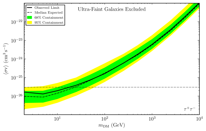
The combined limits presented in Section V include the ultra-faint dwarf galaxies Segue 1, Ursa Major II, and Willman 1. While Bayesian hierarchical modeling sets rather tight constraints on these dwarf galaxies as members of the dwarf galaxy population, the stellar kinematic data yield larger uncertainties on the of these dwarf galaxies when analyzed individually. For example the velocity distribution of Willman 1 appears to be bimodal, and it is not yet clear whether the stars are dynamically bound to this object (Willman et al., 2011). Similarly, the photometry of Ursa Major II shows that this object is elongated; however, the major axis of Ursa Major II does not point in the direction of the Galactic center and it is unclear if this elongation should be interpreted as a sign of tidal disruption (Muñoz et al., 2010). Removing these three ultra-faint dwarf galaxies has a impact on the combined limits for soft annihilation spectra (e.g., models or models with ) and weakens the limits by a factor of for hard annihilation spectra (e.g., models with ); however, it does not significantly impact the constraint on the thermal relic cross section at low dark matter masses (Figure 6). Moreover, as mentioned in Section V, these ultra-faint dwarf galaxies contribute heavily to the excess observed in the combined analysis. The removal of all three ultra-faint galaxies reduces the maximum excess from to . Conversely, forming a composite analysis from just the three ultra-faint dwarf galaxies yields , the significance of which must be decreased by an additional trials factor.
VII Bayesian Analysis
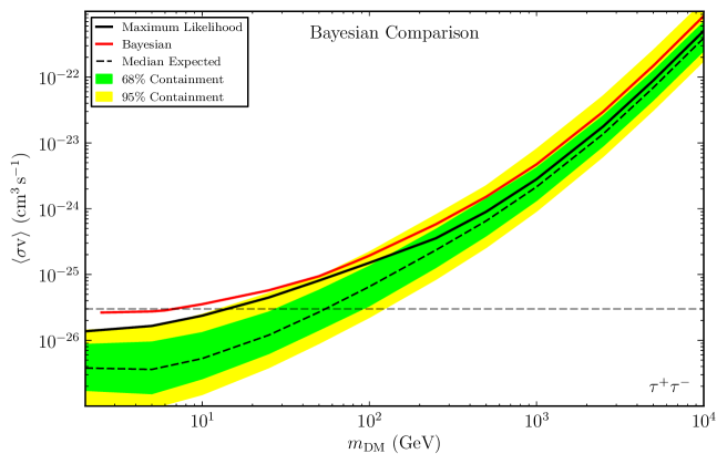
As a further check of the maximum likelihood analysis, we perform a complementary Bayesian analysis based on the technique of Mazziotta et al. (2012). This approach derives the diffuse background empirically from annuli surrounding the dwarf galaxies and incorporates the instrument response through an iterative Bayesian unfolding Abdo et al. (2010d); Loparco and Mazziotta (2009); Mazziotta (2009). The Bayesian method discussed here improves upon that of Mazziotta et al. (2012) by folding the dark matter signal spectrum with the IRFs and incorporating information from all energy bins when reconstructing a posterior probability distribution for the dark matter cross section. We apply this method to our 4-year data sample and derive upper limits on the dark matter annihilation cross section from a combined analysis of the 15 dwarf galaxies selected in Section V.2. We find that the results of the Bayesian and maximum likelihood analyses are comparable despite intrinsically different assumptions and methodologies.
We begin by selecting signal and background regions centered on each of the dwarf galaxies. Signal regions are defined as cones of angular radius,101010The signal region is chosen to correspond to the solid angle used for calculations (Section IV.2). while background regions are defined as annuli with inner radii of and outer radii of . When defining the background regions, all data within of 2FGL catalog sources are masked. Data are binned in energy according to the prescription in Section III.
Within each energy bin we denote the number of counts in the signal region as and the number of counts in the background region as . We assume that the probabilities of measuring counts in the signal region and counts in the background region are both Poisson distributed with expected values and , respectively. Here, is the expected number of signal counts (in the signal region), is the expected number of background counts (in the background region), while is the ratio of solid angles between the signal and background regions.111111Point-source masking is accounted for when calculating the ratio of solid angles between the signal and background regions Mazziotta et al. (2012). The values of are tied across the energy bins by the shape of the putative dark matter spectrum and folded with the LAT instrument response. For each dwarf, the response of the LAT instrument is evaluated from full Monte Carlo simulations of the detector, which take into account the energy dispersion.
Starting from the measured counts in the signal and background regions, we evaluate the Bayesian posterior probability density function (PDF),
| (15) | ||||
Here we indicate with and the counts in the signal and background regions and with the expected counts in the background regions. The likelihood is the product of Poisson probabilities across all energy bins, while , , and are the prior PDFs for the cross section, , and background counts, respectively. Prior PDFs for the cross section and background counts are assumed to be uniform, while the prior PDF for the is assumed to be log-normal with mean and variance taken from Table 1. The posterior PDF on is evaluated from Equation (15), marginalizing the joint PDF over the nuisance parameters and . Upper limits on are calculated by integrating the posterior PDF. We perform a combined analysis of the 15 dwarf galaxies in Section III using a similar technique, weighting the data associated with each source by its [Equation (15)].
We validate the performance of the Bayesian analysis by applying it to random blank fields in the high-latitude data chosen in a manner similar to that described in Section VI. Similar to the maximum likelihood analysis, we find that the observed cross section limits for low dark matter masses are slightly higher than the median expected from random fields, but are consistent within statistical fluctuations. The Bayesian analysis presented here is significantly more sensitive to high-mass dark matter models than that presented in Mazziotta et al. (2012) due to the utilization of all energy bins when testing putative dark matter signal spectra. However, the upper limits derived from the Bayesian analysis are slightly less constraining than those derived from maximum likelihood analysis. The differing results may be ascribed to alternative models of the signal (i.e., finite aperture vs. spatial profile) and of the background (i.e., local annulus vs. global template). Additionally, differences between the delta-log-likelihood method and the Bayesian method for setting upper limits will lead to more conservative Bayesian limits in the low-counts regime. Despite differences in background modeling, the treatment of the LAT instrument performance, and the methodology for setting upper limits, the Bayesian and maximum likelihood analyses yield comparable results (Figure 7).
VIII Conclusions
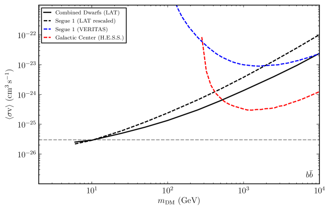
We have reported on 4-year -ray observations of 25 dwarf spheroidal satellite galaxies of the Milky Way. No significant -ray excess was found coincident with any of the dwarf galaxies for any of the spectral models tested. We performed a combined analysis of 15 dwarf galaxies under the assumption that the characteristics of the dark matter particle are shared between the dwarfs. Again, no globally significant excess was found for any of the spectral models tested. We set 95% CL limits on the thermally averaged dark matter annihilation cross section incorporating statistical uncertainties in the derived from fits to stellar kinematic data. These limits constrain the dark matter annihilation cross section to be less than for dark matter particles with a mass less than for the channel and a mass less than for the and channels. Our limits on the dark matter annihilation cross section extend to dark matter masses of , although Imaging Air Cherenkov Telescopes present more constraining limits at high dark matter masses (Figure 8) Aliu et al. (2012); Abramowski et al. (2011); Aleksic et al. (2011).
The analysis presented here greatly improves our understanding of the statistical and systematic issues involved in the search for dwarf spheroidal galaxies. Comparing our results to the 2-year maximum likelihood study of 10 dwarf galaxies by Ackermann et al. (2011), we find that the current limits are a factor of weaker for soft spectral models and a factor of stronger for hard spectral models. These changes can be attributed to updated , the increased photon energy range, the inclusion of more dwarf spheroidal galaxies (specifically Willman 1), and a reclassification of events when moving from Pass 6 to P7REP. As expected, we find that 4 years of P7REP data yield more constraining limits than 2 years of P7REP data.
The largest deviation from the null hypothesis occurs for soft -ray spectra and is fit by dark matter in the mass range from 10 to 25 annihilating to and has . Control studies of random blank sky locations suggest that the global significance of this excess is . This deviation can also be fit by lower mass dark matter () annihilating through harder channels (i.e., ). Much interest in the low-mass WIMP regime has been triggered by -ray studies of the Galactic center (Hooper and Linden, 2011; Abazajian and Kaplinghat, 2012) and by recent direct detection results (Agnese et al., 2013). While suggestive, the analysis of dwarf spheroidal galaxies presented here remains consistent with the null hypothesis within statistical fluctuation. Constraints on the dark matter annihilation cross section derived here are found to be robust against the systematic uncertainties considered; however, systematics associated with the diffuse modeling are found to more significantly impact the derived for the low-mass excess.
Upcoming improvements to the LAT instrument performance and continued data taking will lead to increased sensitivity for dark matter annihilation in dwarf spheroidal galaxies. The novel event reconstruction and event selection of Pass 8 will be especially important as it will both increase the LAT sensitivity to point-like sources and help mitigate systematic effects present in P7REP Atwood et al. (2013). Another exciting prospect is the discovery of new dwarf spheroidal galaxies. Over the past ten years, data from the Sloan Digital Sky Survey (SDSS) (Abazajian et al., 2009) have been used to roughly double the number of known dwarf spheroidal galaxies, while only covering of the sky (Willman, 2010). Thus, the next generations of deep, wide-field photometric surveys (e.g., PanSTARRS (Kaiser et al., 2002), Southern Sky Survey (Keller et al., 2007), DES (Abbott et al., 2005), and LSST (Ivezic et al., 2008)) are expected to greatly increase the number of known Milky Way dwarf spheroidal satellite galaxies Tollerud et al. (2008). The discovery and characterization of new dwarf spheroidal galaxies could greatly improve the LAT sensitivity to dark matter annihilation in this class of objects.
IX Acknowledgments
The Fermi-LAT Collaboration acknowledges generous ongoing support from a number of agencies and institutes that have supported both the development and the operation of the LAT as well as scientific data analysis. These include the National Aeronautics and Space Administration and the Department of Energy in the United States, the Commissariat à l’Energie Atomique and the Centre National de la Recherche Scientifique / Institut National de Physique Nucléaire et de Physique des Particules in France, the Agenzia Spaziale Italiana and the Istituto Nazionale di Fisica Nucleare in Italy, the Ministry of Education, Culture, Sports, Science and Technology (MEXT), High Energy Accelerator Research Organization (KEK) and Japan Aerospace Exploration Agency (JAXA) in Japan, and the K. A. Wallenberg Foundation, the Swedish Research Council and the Swedish National Space Board in Sweden.
Additional support for science analysis during the operations phase is gratefully acknowledged from the Istituto Nazionale di Astrofisica in Italy and the Centre National d’Études Spatiales in France.
Support was also provided by the Department of Energy Office of Science Graduate Fellowship Program (DOE SCGF) administered by ORISE-ORAU under Contract No. DE-AC05-06OR23100 and by the Wenner-Gren Foundation. J.C. is a Wallenberg Academy Fellow, supported by the Knut and Alice Wallenberg foundation. M.R. received funds from contract FIRB-2012-RBFR12PM1F from the Italian Ministry of Education, University and Research (MIUR). The authors would like to thank Joakim Edsjö, Torbjörn Sjöstrand, and Peter Skands for helpful conversations concerning Pythia. The authors acknowledge the use of HEALPix Górski et al. (2005).121212http://healpix.sourceforge.net
References
- Ade et al. (2013) P. Ade et al. (Planck Collaboration), (2013), arXiv:1303.5076 [astro-ph.CO] .
- Jungman et al. (1996) G. Jungman, M. Kamionkowski, and K. Griest, Phys. Rep. 267, 195 (1996), arXiv:hep-ph/9506380 [hep-ph] .
- Bergstrom (2000) L. Bergstrom, Rept. Prog. Phys. 63, 793 (2000), arXiv:hep-ph/0002126 [hep-ph] .
- Bertone et al. (2005) G. Bertone, D. Hooper, and J. Silk, Phys. Rep. 405, 279 (2005), arXiv:hep-ph/0404175 [hep-ph] .
- Steigman et al. (2012) G. Steigman, B. Dasgupta, and J. F. Beacom, Phys.Rev. D86, 023506 (2012), arXiv:1204.3622 [hep-ph] .
- Atwood et al. (2009) W. Atwood et al. (Fermi-LAT Collaboration), ApJ 697, 1071 (2009), arXiv:0902.1089 [astro-ph.IM] .
- Hooper and Linden (2011) D. Hooper and T. Linden, Phys.Rev. D84, 123005 (2011), arXiv:1110.0006 [astro-ph.HE] .
- Ackermann et al. (2012a) M. Ackermann et al. (Fermi-LAT Collaboration), ApJ 761, 91 (2012a), arXiv:1205.6474 [astro-ph.CO] .
- Abazajian and Kaplinghat (2012) K. N. Abazajian and M. Kaplinghat, Phys.Rev. D86, 083511 (2012), arXiv:1207.6047 [astro-ph.HE] .
- Abdo et al. (2010a) A. Abdo et al., Phys. Rev. Lett. 104, 091302 (2010a), arXiv:1001.4836 [astro-ph.HE] .
- Ackermann et al. (2012b) M. Ackermann et al. (Fermi-LAT Collaboration), Phys.Rev. D86, 022002 (2012b), arXiv:1205.2739 [astro-ph.HE] .
- Weniger (2012) C. Weniger, JCAP 1208, 007 (2012), arXiv:1204.2797 [hep-ph] .
- Ackermann et al. (2013a) M. Ackermann et al. (Fermi-LAT Collaboration), (2013a), arXiv:1305.5597 [astro-ph.HE] .
- Abdo et al. (2010b) A. Abdo et al. (Fermi-LAT Collaboration), J. Cosmology Astropart. Phys 1004, 014 (2010b), arXiv:1002.4415 [astro-ph.CO] .
- Abazajian et al. (2010) K. N. Abazajian, P. Agrawal, Z. Chacko, and C. Kilic, JCAP 1011, 041 (2010), arXiv:1002.3820 [astro-ph.HE] .
- Ackermann et al. (2010) M. Ackermann et al., J. Cosmology Astropart. Phys 1005, 025 (2010), arXiv:1002.2239 [astro-ph.CO] .
- Zechlin et al. (2012) H. Zechlin, M. Fernandes, D. Elsaesser, and D. Horns, Astron.Astrophys. 538, A93 (2012), arXiv:1111.3514 [astro-ph.HE] .
- Ackermann et al. (2012c) M. Ackermann et al. (Fermi-LAT Collaboration), ApJ 747, 121 (2012c), arXiv:1201.2691 [astro-ph.HE] .
- Zechlin and Horns (2012) H.-S. Zechlin and D. Horns, JCAP 1211, 050 (2012), arXiv:1210.3852 [astro-ph.HE] .
- Abdo et al. (2010c) A. Abdo et al. (Fermi-LAT Collaboration), ApJ 712, 147 (2010c), arXiv:1001.4531 [astro-ph.CO] .
- Ackermann et al. (2011) M. Ackermann et al. (Fermi-LAT Collaboration), Phys. Rev. Lett. 107, 241302 (2011), arXiv:1108.3546 [astro-ph.HE] .
- Geringer-Sameth and Koushiappas (2011) A. Geringer-Sameth and S. M. Koushiappas, Phys.Rev.Lett. 107, 241303 (2011), arXiv:1108.2914 [astro-ph.CO] .
- Mazziotta et al. (2012) M. N. Mazziotta, F. Loparco, F. de Palma, and N. Giglietto, Astropart. 37, 26 (2012), arXiv:1203.6731 [astro-ph.IM] .
- Geringer-Sameth and Koushiappas (2012) A. Geringer-Sameth and S. M. Koushiappas, Phys.Rev. D86, 021302 (2012), arXiv:1206.0796 [astro-ph.HE] .
- Mateo (1998) M. Mateo, Ann.Rev.Astron.Astrophys. 36, 435 (1998), arXiv:astro-ph/9810070 [astro-ph] .
- Grcevich and Putman (2009) J. Grcevich and M. E. Putman, ApJ 696, 385 (2009), arXiv:0901.4975 [astro-ph.GA] .
- Nolan et al. (2012) P. Nolan et al. (Fermi-LAT Collaboration), ApJS 199, 31 (2012), arXiv:1108.1435 [astro-ph.HE] .
- Ackermann et al. (2012d) M. Ackermann et al. (Fermi-LAT Collaboration), ApJS 203, 4 (2012d), arXiv:1206.1896 [astro-ph.IM] .
- Bregeon et al. (2013) J. Bregeon et al. (Fermi-LAT Collaboration), (2013), arXiv:1304.5456 [astro-ph.HE] .
- Ackermann et al. (2013b) M. Ackermann et al., (2013b), in preparation.
- Abdo et al. (2010d) A. Abdo et al. (Fermi-LAT Collaboration), ApJ 716, 30 (2010d), arXiv:0912.2040 [astro-ph.CO] .
- Bartlett (1953) M. Bartlett, Biometrika 40, 306 (1953).
- Rolke et al. (2005) W. A. Rolke, A. M. Lopez, and J. Conrad, Nucl.Instrum.Meth. A551, 493 (2005), arXiv:physics/0403059 [physics] .
- Charbonnier et al. (2011) A. Charbonnier, C. Combet, M. Daniel, S. Funk, J. Hinton, et al., MNRAS 418, 1526 (2011), arXiv:1104.0412 [astro-ph.HE] .
- Jeltema and Profumo (2008) T. E. Jeltema and S. Profumo, JCAP 0811, 003 (2008), arXiv:0808.2641 [astro-ph] .
- Sjöstrand et al. (2006) T. Sjöstrand, S. Mrenna, and P. Z. Skands, JHEP 0605, 026 (2006), arXiv:hep-ph/0603175 [hep-ph] .
- Sjöstrand et al. (2008) T. Sjöstrand, S. Mrenna, and P. Z. Skands, Comput.Phys.Commun. 178, 852 (2008), arXiv:0710.3820 [hep-ph] .
- Essig et al. (2009) R. Essig, N. Sehgal, and L. E. Strigari, Phys. Rev. D 80, 023506 (2009), arXiv:0902.4750 [hep-ph] .
- Beacom et al. (2005) J. F. Beacom, N. F. Bell, and G. Bertone, Phys. Rev. Lett. 94, 171301 (2005), arXiv:astro-ph/0409403 [astro-ph] .
- Birkedal et al. (2005) A. Birkedal, K. T. Matchev, M. Perelstein, and A. Spray, (2005), arXiv:hep-ph/0507194 [hep-ph] .
- Mardon et al. (2009) J. Mardon, Y. Nomura, D. Stolarski, and J. Thaler, JCAP 0905, 016 (2009), arXiv:0901.2926 [hep-ph] .
- Battaglia et al. (2013) G. Battaglia, A. Helmi, and M. Breddels, (2013), arXiv:1305.5965 [astro-ph.CO] .
- Walker et al. (2009) M. G. Walker, M. Mateo, E. W. Olszewski, J. Penarrubia, N. Evans, et al., ApJ 704, 1274 (2009), arXiv:0906.0341 [astro-ph.CO] .
- Wolf et al. (2010) J. Wolf, G. D. Martinez, J. S. Bullock, M. Kaplinghat, M. Geha, et al., MNRAS 406, 1220 (2010), arXiv:0908.2995 [astro-ph.CO] .
- Martinez et al. (2009) G. D. Martinez, J. S. Bullock, M. Kaplinghat, L. E. Strigari, and R. Trotta, JCAP 0906, 014 (2009), arXiv:0902.4715 [astro-ph.HE] .
- Strigari (2013) L. E. Strigari, Physics Reports , 1 (2013), arXiv:1211.7090 [astro-ph.CO] .
- Martinez (2013) G. D. Martinez, (2013), arXiv:1309.2641 [astro-ph.GA] .
- Dall’Ora et al. (2006) M. Dall’Ora, G. Clementini, K. Kinemuchi, V. Ripepi, M. Marconi, et al., ApJ 653, L109 (2006), arXiv:astro-ph/0611285 [astro-ph] .
- Simon and Geha (2007) J. D. Simon and M. Geha, ApJ 670, 313 (2007), arXiv:0706.0516 [astro-ph] .
- Walker et al. (2009) M. G. Walker, M. Mateo, and E. W. Olszewski, AJ 137, 3100 (2009), arXiv:0811.0118 .
- Mateo et al. (2008) M. Mateo, E. W. Olszewski, and M. G. Walker, ApJ 675, 201 (2008), arXiv:0708.1327 [astro-ph] .
- Koch et al. (2007) A. Koch, J. Kleyna, M. Wilkinson, E. Grebel, G. Gilmore, et al., AJ 134, 566 (2007), arXiv:0704.3437 [astro-ph] .
- Simon et al. (2011) J. D. Simon, M. Geha, Q. E. Minor, G. D. Martinez, E. N. Kirby, et al., ApJ 733, 46 (2011), arXiv:1007.4198 [astro-ph.GA] .
- Muñoz et al. (2005) R. R. Muñoz, P. M. Frinchaboy, S. R. Majewski, J. R. Kuhn, M.-Y. Chou, et al., ApJ 631, L137 (2005), arXiv:astro-ph/0504035 [astro-ph] .
- Willman et al. (2011) B. Willman, M. Geha, J. Strader, L. E. Strigari, J. D. Simon, E. Kirby, N. Ho, and A. Warres, AJ 142, 128 (2011), arXiv:1007.3499 [astro-ph.GA] .
- Strigari et al. (2008a) L. E. Strigari, J. S. Bullock, M. Kaplinghat, J. D. Simon, M. Geha, et al., Nature 454, 1096 (2008a), 0808.3772 [astro-ph] .
- Loredo and Hendry (2009) T. J. Loredo and M. A. Hendry, Bayesian Methods in Cosmology, edited by M. P. Hobson, A. H. Jaffe, A. R. Liddle, P. Mukherjee, and D. Parkinson (Cambridge University Press, 2009).
- Springel et al. (2008) V. Springel, J. Wang, M. Vogelsberger, A. Ludlow, A. Jenkins, et al., MNRAS 391, 1685 (2008), arXiv:0809.0898 [astro-ph] .
- Diemand et al. (2007) J. Diemand, M. Kuhlen, and P. Madau, ApJ 657, 262 (2007), arXiv:astro-ph/0611370 [astro-ph] .
- Koposov et al. (2008) S. Koposov, V. Belokurov, N. Evans, P. Hewett, M. Irwin, et al., ApJ 686, 279 (2008), arXiv:0706.2687 [astro-ph] .
- Skilling (2004) J. Skilling, in American Institute of Physics Conference Series, American Institute of Physics Conference Series, Vol. 735, edited by R. Fischer, R. Preuss, and U. V. Toussaint (2004) pp. 395–405.
- Gilmore et al. (2007) G. Gilmore, M. I. Wilkinson, R. F. Wyse, J. T. Kleyna, A. Koch, et al., ApJ 663, 948 (2007), arXiv:astro-ph/0703308 [ASTRO-PH] .
- Strigari et al. (2010) L. E. Strigari, C. S. Frenk, and S. D. White, MNRAS 408, 2364 (2010), arXiv:1003.4268 [astro-ph.CO] .
- Walker and Penarrubia (2011) M. G. Walker and J. Penarrubia, ApJ 742, 20 (2011), arXiv:1108.2404 [astro-ph.CO] .
- Agnello and Evans (2012) A. Agnello and N. Evans, ApJ 754, L39 (2012), arXiv:1205.6673 [astro-ph.GA] .
- Navarro et al. (1997) J. F. Navarro, C. S. Frenk, and S. D. White, ApJ 490, 493 (1997), arXiv:astro-ph/9611107 [astro-ph] .
- Burkert (1995) A. Burkert, ApJ 447, 25 (1995), arXiv:astro-ph/9504041 [astro-ph] .
- Strigari et al. (2008b) L. E. Strigari, S. M. Koushiappas, J. S. Bullock, M. Kaplinghat, J. D. Simon, et al., ApJ 678, 614 (2008b), arXiv:0709.1510 [astro-ph] .
- Mattox et al. (1996) J. Mattox, D. Bertsch, J. Chiang, B. Dingus, S. Digel, et al., ApJ 461, 396 (1996).
- Chernoff (1954) H. Chernoff, Ann. Math. Statist. 25, 573 (1954).
- Su et al. (2010) M. Su, T. R. Slatyer, and D. P. Finkbeiner, ApJ 724, 1044 (2010), arXiv:1005.5480 [astro-ph.HE] .
- Su and Finkbeiner (2012) M. Su and D. P. Finkbeiner, ApJ 753, 61 (2012), arXiv:1205.5852 [astro-ph.HE] .
- Aharonian et al. (2008) F. Aharonian et al. (HESS Collaboration), Astropart.Phys. 29, 55 (2008), arXiv:0711.2369 [astro-ph] .
- Frinchaboy et al. (2012) P. M. Frinchaboy, S. R. Majewski, R. R. Munoz, D. R. Law, E. L. Lokas, et al., ApJ 756, 74 (2012), arXiv:1207.3346 [astro-ph.GA] .
- Demortier (2003) L. Demortier, PHYSTAT 2003 Proceedings, eConf C030908, WEMT003 (2003), arXiv:physics/0312100 [physics] .
- Gross (2011) E. Gross (ATLAS Collaboration), “Frequentist Limit Recommendation,” ATLAS Statistics Forum (2011).
- James and Roos (1975) F. James and M. Roos, Comput.Phys.Commun. 10, 343 (1975).
- de Palma et al. (2013) F. de Palma, T. Brandt, G. Johannesson, and L. Tibaldo (Fermi-LAT Collaboration), 2012 Fermi Symposium Proceedings, eConf C121028 (2013), arXiv:1304.1395 [astro-ph.HE] .
- Ackermann et al. (2012e) M. Ackermann et al. (Fermi-LAT Collaboration), ApJ 750, 3 (2012e), arXiv:1202.4039 [astro-ph.HE] .
- Casandjian and Grenier (2009) J.-M. Casandjian and I. Grenier (Fermi-LAT Collaboration), 2009 Fermi Symposium Proceedings, eConf C091122 (2009), arXiv:0912.3478 [astro-ph.HE] .
- Wolleben (2007) M. Wolleben, ApJ 664, 349 (2007), arXiv:0704.0276 [astro-ph] .
- Muñoz et al. (2010) R. R. Muñoz, M. Geha, and B. Willman, AJ 140, 138 (2010), arXiv:0910.3946 [astro-ph.GA] .
- Loparco and Mazziotta (2009) F. Loparco and M. N. Mazziotta (Fermi-LAT Collaboration), 2009 Fermi Symposium Proceedings, eConf C091122 (2009), arXiv:0912.3695 [astro-ph.IM] .
- Mazziotta (2009) M. N. Mazziotta (Fermi-LAT Collaboration), 31st ICRC Proceedings, (2009), arXiv:0912.1236 [astro-ph.IM] .
- Aliu et al. (2012) E. Aliu et al. (VERITAS Collaboration), Phys.Rev. D85, 062001 (2012), arXiv:1202.2144 [astro-ph.HE] .
- Abramowski et al. (2011) A. Abramowski et al. (H.E.S.S.Collaboration), Phys.Rev.Lett. 106, 161301 (2011), arXiv:1103.3266 [astro-ph.HE] .
- Aleksic et al. (2011) J. Aleksic et al. (MAGIC Collaboration), JCAP 1106, 035 (2011), arXiv:1103.0477 [astro-ph.HE] .
- Agnese et al. (2013) R. Agnese et al. (CDMS Collaboration), (2013), arXiv:1304.4279 [hep-ex] .
- Atwood et al. (2013) W. Atwood et al. (Fermi-LAT Collaboration), 2012 Fermi Symposium Proceedings, eConf C121028 (2013), arXiv:1303.3514 [astro-ph.IM] .
- Abazajian et al. (2009) K. N. Abazajian et al. (SDSS Collaboration), ApJS 182, 543 (2009), arXiv:0812.0649 [astro-ph] .
- Willman (2010) B. Willman, Adv.Astron. 2010, 1 (2010), arXiv:0907.4758 [astro-ph.CO] .
- Kaiser et al. (2002) N. Kaiser, H. Aussel, H. Boesgaard, K. Chambers, J. N. Heasley, et al., Proc.SPIE Int.Soc.Opt.Eng. 4836, 154 (2002).
- Keller et al. (2007) S. Keller, B. Schmidt, and M. Bessell, PASA 24, 1 (2007), arXiv:0704.1339 [astro-ph] .
- Abbott et al. (2005) T. Abbott et al. (DES Collaboration), (2005), arXiv:astro-ph/0510346 [astro-ph] .
- Ivezic et al. (2008) Z. Ivezic, J. Tyson, R. Allsman, J. Andrew, and R. Angel (LSST Collaboration), (2008), arXiv:0805.2366 [astro-ph] .
- Tollerud et al. (2008) E. J. Tollerud, J. S. Bullock, L. E. Strigari, and B. Willman, ApJ 688, 277 (2008), arXiv:0806.4381 [astro-ph] .
- Górski et al. (2005) K. M. Górski, E. Hivon, A. J. Banday, B. D. Wandelt, F. K. Hansen, M. Reinecke, and M. Bartelmann, ApJ 622, 759 (2005), arXiv:astro-ph/0409513 .
X Figures & Tables
| Name | GLON | GLAT | Distance | 111 are calculated over a solid angle of . | 111 are calculated over a solid angle of . | Reference | ||
| () | () | () | () | () | () | () | ||
| Bootes I | 358.1 | 69.6 | 66 | Dall’Ora et al. (2006) | ||||
| Bootes II | 353.7 | 68.9 | 42 | – | – | – | – | – |
| Bootes III | 35.4 | 75.4 | 47 | – | – | – | – | – |
| Canes Venatici I | 74.3 | 79.8 | 218 | Simon and Geha (2007) | ||||
| Canes Venatici II | 113.6 | 82.7 | 160 | Simon and Geha (2007) | ||||
| Canis Major | 240.0 | -8.0 | 7 | – | – | – | – | – |
| Carina | 260.1 | -22.2 | 105 | Walker et al. (2009) | ||||
| Coma Berenices | 241.9 | 83.6 | 44 | Simon and Geha (2007) | ||||
| Draco | 86.4 | 34.7 | 76 | Muñoz et al. (2005) | ||||
| Fornax | 237.1 | -65.7 | 147 | Walker et al. (2009) | ||||
| Hercules | 28.7 | 36.9 | 132 | Simon and Geha (2007) | ||||
| Leo I | 226.0 | 49.1 | 254 | Mateo et al. (2008) | ||||
| Leo II | 220.2 | 67.2 | 233 | Koch et al. (2007) | ||||
| Leo IV | 265.4 | 56.5 | 154 | Simon and Geha (2007) | ||||
| Leo V | 261.9 | 58.5 | 178 | – | – | – | – | – |
| Pisces II | 79.2 | -47.1 | 182 | – | – | – | – | – |
| Sagittarius | 5.6 | -14.2 | 26 | – | – | – | – | – |
| Sculptor | 287.5 | -83.2 | 86 | Walker et al. (2009) | ||||
| Segue 1 | 220.5 | 50.4 | 23 | Simon et al. (2011) | ||||
| Segue 2 | 149.4 | -38.1 | 35 | – | – | – | – | – |
| Sextans | 243.5 | 42.3 | 86 | Walker et al. (2009) | ||||
| Ursa Major I | 159.4 | 54.4 | 97 | Simon and Geha (2007) | ||||
| Ursa Major II | 152.5 | 37.4 | 32 | Simon and Geha (2007) | ||||
| Ursa Minor | 105.0 | 44.8 | 76 | Muñoz et al. (2005) | ||||
| Willman 1 | 158.6 | 56.8 | 38 | Willman et al. (2011) | ||||
| 2 | 5 | 10 | 25 | 50 | 100 | 250 | 500 | 1000 | 2500 | 5000 | 10000 | |
|---|---|---|---|---|---|---|---|---|---|---|---|---|
| Bootes I | 1.49e-25 | 2.12e-25 | 3.26e-25 | 1.68e-24 | 3.80e-24 | 9.81e-24 | 3.74e-23 | 1.09e-22 | 3.71e-22 | 2.01e-21 | 7.45e-21 | 2.82e-20 |
| Bootes II | – | – | – | – | – | – | – | – | – | – | – | – |
| Bootes III | – | – | – | – | – | – | – | – | – | – | – | – |
| Canes Venatici I | 1.35e-24 | 1.20e-24 | 5.51e-24 | 1.51e-23 | 3.58e-23 | 9.33e-23 | 4.18e-22 | 1.28e-21 | 4.46e-21 | 2.47e-20 | 9.23e-20 | 3.50e-19 |
| Canes Venatici II | 2.42e-24 | 2.21e-24 | 3.16e-24 | 5.42e-24 | 1.20e-23 | 3.05e-23 | 1.23e-22 | 3.84e-22 | 1.34e-21 | 7.47e-21 | 2.79e-20 | 1.06e-19 |
| Canis Major | – | – | – | – | – | – | – | – | – | – | – | – |
| Carina | 1.06e-24 | 9.76e-25 | 9.94e-25 | 2.10e-24 | 4.99e-24 | 3.65e-23 | 1.54e-22 | 4.86e-22 | 1.71e-21 | 9.53e-21 | 3.57e-20 | 1.35e-19 |
| Coma Berenices | 7.90e-26 | 8.25e-26 | 1.43e-25 | 3.72e-25 | 8.71e-25 | 2.34e-24 | 9.75e-24 | 3.08e-23 | 1.09e-22 | 6.05e-22 | 2.26e-21 | 8.60e-21 |
| Draco | 6.26e-26 | 1.41e-25 | 2.11e-25 | 5.23e-25 | 1.35e-24 | 3.21e-24 | 1.18e-23 | 3.46e-23 | 1.19e-22 | 6.49e-22 | 2.41e-21 | 9.14e-21 |
| Fornax | 3.76e-25 | 1.05e-24 | 1.43e-24 | 3.80e-24 | 1.01e-23 | 2.34e-23 | 8.50e-23 | 2.49e-22 | 8.53e-22 | 4.66e-21 | 1.73e-20 | 6.56e-20 |
| Hercules | 2.33e-24 | 3.34e-24 | 7.95e-24 | 1.71e-23 | 3.40e-23 | 7.75e-23 | 2.68e-22 | 7.54e-22 | 2.51e-21 | 1.34e-20 | 4.96e-20 | 1.87e-19 |
| Leo I | 1.75e-24 | 3.14e-24 | 4.01e-24 | 9.14e-24 | 1.90e-23 | 5.03e-23 | 2.19e-22 | 6.79e-22 | 2.38e-21 | 1.32e-20 | 4.93e-20 | 1.87e-19 |
| Leo II | 2.78e-24 | 1.80e-24 | 2.26e-24 | 5.52e-24 | 1.48e-23 | 4.12e-23 | 1.79e-22 | 5.74e-22 | 2.03e-21 | 1.14e-20 | 4.26e-20 | 1.62e-19 |
| Leo IV | 5.89e-25 | 7.87e-25 | 1.22e-24 | 3.42e-24 | 8.82e-24 | 2.54e-23 | 1.13e-22 | 3.68e-22 | 1.31e-21 | 7.37e-21 | 2.77e-20 | 1.05e-19 |
| Leo V | – | – | – | – | – | – | – | – | – | – | – | – |
| Pisces II | – | – | – | – | – | – | – | – | – | – | – | – |
| Sagittarius | – | – | – | – | – | – | – | – | – | – | – | – |
| Sculptor | 1.36e-25 | 3.24e-25 | 1.16e-24 | 2.76e-24 | 5.98e-24 | 1.36e-23 | 4.64e-23 | 1.27e-22 | 4.23e-22 | 2.27e-21 | 8.39e-21 | 3.17e-20 |
| Segue 1 | 7.38e-26 | 9.73e-26 | 2.81e-25 | 7.46e-25 | 1.57e-24 | 3.85e-24 | 1.30e-23 | 3.46e-23 | 1.13e-22 | 5.97e-22 | 2.19e-21 | 8.25e-21 |
| Segue 2 | – | – | – | – | – | – | – | – | – | – | – | – |
| Sextans | 1.18e-24 | 7.97e-25 | 9.34e-25 | 1.76e-24 | 3.94e-24 | 1.04e-23 | 4.32e-23 | 1.39e-22 | 4.91e-22 | 2.75e-21 | 1.03e-20 | 3.92e-20 |
| Ursa Major I | 1.35e-25 | 2.96e-25 | 5.08e-25 | 1.24e-24 | 3.02e-24 | 9.20e-24 | 3.79e-23 | 1.18e-22 | 4.13e-22 | 2.29e-21 | 8.57e-21 | 3.25e-20 |
| Ursa Major II | 9.92e-26 | 1.49e-25 | 2.73e-25 | 3.92e-25 | 6.69e-25 | 2.42e-24 | 8.47e-24 | 2.41e-23 | 8.20e-23 | 4.45e-22 | 1.65e-21 | 6.24e-21 |
| Ursa Minor | 5.80e-26 | 8.27e-26 | 1.30e-25 | 4.03e-25 | 9.83e-25 | 2.50e-24 | 9.78e-24 | 2.98e-23 | 1.03e-22 | 5.71e-22 | 2.13e-21 | 8.08e-21 |
| Willman 1 | 2.00e-25 | 2.79e-25 | 4.52e-25 | 1.10e-24 | 2.65e-24 | 6.45e-24 | 2.36e-23 | 6.81e-23 | 2.29e-22 | 1.23e-21 | 4.56e-21 | 1.72e-20 |
| Combined | 4.24e-26 | 5.07e-26 | 1.03e-25 | 2.16e-25 | 3.71e-25 | 8.71e-25 | 2.26e-24 | 5.68e-24 | 1.85e-23 | 9.78e-23 | 3.59e-22 | 1.35e-21 |
| 2 | 5 | 10 | 25 | 50 | 100 | 250 | 500 | 1000 | 2500 | 5000 | 10000 | |
|---|---|---|---|---|---|---|---|---|---|---|---|---|
| Bootes I | 3.59e-25 | 5.05e-25 | 6.64e-25 | 2.64e-24 | 5.69e-24 | 1.39e-23 | 5.04e-23 | 1.43e-22 | 4.59e-22 | 2.36e-21 | 8.49e-21 | 3.14e-20 |
| Bootes II | – | – | – | – | – | – | – | – | – | – | – | – |
| Bootes III | – | – | – | – | – | – | – | – | – | – | – | – |
| Canes Venatici I | 3.66e-24 | 2.74e-24 | 9.59e-24 | 2.38e-23 | 5.35e-23 | 1.32e-22 | 5.44e-22 | 1.62e-21 | 5.40e-21 | 2.86e-20 | 1.04e-19 | 3.89e-19 |
| Canes Venatici II | 6.31e-24 | 5.51e-24 | 6.77e-24 | 9.63e-24 | 1.87e-23 | 4.39e-23 | 1.64e-22 | 4.87e-22 | 1.62e-21 | 8.62e-21 | 3.15e-20 | 1.18e-19 |
| Canis Major | – | – | – | – | – | – | – | – | – | – | – | – |
| Carina | 2.81e-24 | 2.53e-24 | 2.10e-24 | 3.57e-24 | 7.57e-24 | 4.99e-23 | 1.99e-22 | 6.09e-22 | 2.05e-21 | 1.10e-20 | 4.02e-20 | 1.50e-19 |
| Coma Berenices | 2.02e-25 | 1.77e-25 | 2.61e-25 | 6.01e-25 | 1.31e-24 | 3.28e-24 | 1.28e-23 | 3.88e-23 | 1.30e-22 | 6.96e-22 | 2.55e-21 | 9.54e-21 |
| Draco | 1.87e-25 | 2.83e-25 | 3.88e-25 | 8.60e-25 | 2.00e-24 | 4.61e-24 | 1.60e-23 | 4.49e-23 | 1.46e-22 | 7.57e-22 | 2.74e-21 | 1.02e-20 |
| Fornax | 9.70e-25 | 2.21e-24 | 2.81e-24 | 6.30e-24 | 1.49e-23 | 3.37e-23 | 1.15e-22 | 3.23e-22 | 1.05e-21 | 5.43e-21 | 1.97e-20 | 7.31e-20 |
| Hercules | 6.53e-24 | 7.46e-24 | 1.49e-23 | 2.93e-23 | 5.47e-23 | 1.17e-22 | 3.77e-22 | 1.02e-21 | 3.17e-21 | 1.59e-20 | 5.69e-20 | 2.09e-19 |
| Leo I | 5.62e-24 | 7.04e-24 | 8.27e-24 | 1.54e-23 | 2.96e-23 | 7.14e-23 | 2.88e-22 | 8.58e-22 | 2.87e-21 | 1.52e-20 | 5.56e-20 | 2.08e-19 |
| Leo II | 8.61e-24 | 4.91e-24 | 4.55e-24 | 9.03e-24 | 2.15e-23 | 5.64e-23 | 2.31e-22 | 7.14e-22 | 2.43e-21 | 1.30e-20 | 4.79e-20 | 1.79e-19 |
| Leo IV | 1.87e-24 | 1.65e-24 | 2.24e-24 | 5.38e-24 | 1.28e-23 | 3.46e-23 | 1.44e-22 | 4.55e-22 | 1.56e-21 | 8.43e-21 | 3.10e-20 | 1.16e-19 |
| Leo V | – | – | – | – | – | – | – | – | – | – | – | – |
| Pisces II | – | – | – | – | – | – | – | – | – | – | – | – |
| Sagittarius | – | – | – | – | – | – | – | – | – | – | – | – |
| Sculptor | 3.99e-25 | 7.06e-25 | 2.07e-24 | 4.55e-24 | 9.38e-24 | 2.06e-23 | 6.63e-23 | 1.72e-22 | 5.34e-22 | 2.69e-21 | 9.61e-21 | 3.55e-20 |
| Segue 1 | 1.84e-25 | 2.27e-25 | 5.06e-25 | 1.24e-24 | 2.48e-24 | 5.71e-24 | 1.85e-23 | 4.79e-23 | 1.45e-22 | 7.13e-22 | 2.53e-21 | 9.28e-21 |
| Segue 2 | – | – | – | – | – | – | – | – | – | – | – | – |
| Sextans | 2.97e-24 | 2.12e-24 | 2.02e-24 | 3.03e-24 | 6.08e-24 | 1.47e-23 | 5.67e-23 | 1.74e-22 | 5.88e-22 | 3.16e-21 | 1.16e-20 | 4.34e-20 |
| Ursa Major I | 3.80e-25 | 6.19e-25 | 9.30e-25 | 2.01e-24 | 4.50e-24 | 1.26e-23 | 4.94e-23 | 1.48e-22 | 4.97e-22 | 2.64e-21 | 9.66e-21 | 3.61e-20 |
| Ursa Major II | 2.64e-25 | 3.55e-25 | 5.52e-25 | 7.49e-25 | 1.13e-24 | 3.50e-24 | 1.16e-23 | 3.17e-23 | 1.01e-22 | 5.21e-22 | 1.88e-21 | 6.96e-21 |
| Ursa Minor | 1.61e-25 | 1.65e-25 | 2.34e-25 | 6.22e-25 | 1.45e-24 | 3.53e-24 | 1.30e-23 | 3.80e-23 | 1.25e-22 | 6.62e-22 | 2.41e-21 | 8.98e-21 |
| Willman 1 | 5.43e-25 | 6.50e-25 | 9.06e-25 | 1.85e-24 | 4.07e-24 | 9.44e-24 | 3.26e-23 | 9.08e-23 | 2.87e-22 | 1.46e-21 | 5.21e-21 | 1.93e-20 |
| Combined | 1.16e-25 | 1.22e-25 | 2.01e-25 | 3.77e-25 | 6.33e-25 | 1.38e-24 | 3.38e-24 | 7.92e-24 | 2.37e-23 | 1.17e-22 | 4.13e-22 | 1.52e-21 |
| 2 | 5 | 10 | 25 | 50 | 100 | 250 | 500 | 1000 | 2500 | 5000 | 10000 | |
|---|---|---|---|---|---|---|---|---|---|---|---|---|
| Bootes I | 4.04e-26 | 6.74e-26 | 9.99e-26 | 2.17e-25 | 6.34e-25 | 1.78e-24 | 7.46e-24 | 2.19e-23 | 6.71e-23 | 4.02e-22 | 2.01e-21 | 1.15e-20 |
| Bootes II | – | – | – | – | – | – | – | – | – | – | – | – |
| Bootes III | – | – | – | – | – | – | – | – | – | – | – | – |
| Canes Venatici I | 5.54e-25 | 4.20e-25 | 7.48e-25 | 2.62e-24 | 6.66e-24 | 1.78e-23 | 6.86e-23 | 2.22e-22 | 8.41e-22 | 6.05e-21 | 3.17e-20 | 1.81e-19 |
| Canes Venatici II | 5.25e-25 | 8.30e-25 | 9.41e-25 | 1.15e-24 | 2.00e-24 | 4.86e-24 | 2.16e-23 | 7.62e-23 | 2.97e-22 | 2.17e-21 | 1.12e-20 | 6.21e-20 |
| Canis Major | – | – | – | – | – | – | – | – | – | – | – | – |
| Carina | 2.87e-25 | 4.24e-25 | 3.54e-25 | 4.10e-25 | 8.23e-25 | 3.96e-24 | 2.90e-23 | 1.06e-22 | 4.15e-22 | 2.98e-21 | 1.52e-20 | 8.25e-20 |
| Coma Berenices | 3.15e-26 | 2.26e-26 | 2.99e-26 | 7.01e-26 | 1.61e-25 | 4.24e-25 | 1.88e-24 | 6.58e-24 | 2.55e-23 | 1.85e-22 | 9.56e-22 | 5.25e-21 |
| Draco | 3.35e-26 | 1.95e-26 | 4.18e-26 | 1.04e-25 | 2.26e-25 | 5.78e-25 | 2.23e-24 | 6.80e-24 | 2.37e-23 | 1.59e-22 | 8.12e-22 | 4.53e-21 |
| Fornax | 1.94e-25 | 2.37e-25 | 3.51e-25 | 7.10e-25 | 1.47e-24 | 4.01e-24 | 1.65e-23 | 5.05e-23 | 1.74e-22 | 1.16e-21 | 5.86e-21 | 3.26e-20 |
| Hercules | 7.94e-25 | 8.17e-25 | 1.39e-24 | 3.52e-24 | 6.82e-24 | 1.42e-23 | 4.23e-23 | 1.03e-22 | 3.20e-22 | 2.09e-21 | 1.10e-20 | 6.56e-20 |
| Leo I | 9.35e-25 | 8.84e-25 | 1.10e-24 | 1.70e-24 | 3.34e-24 | 8.25e-24 | 3.83e-23 | 1.41e-22 | 5.51e-22 | 3.90e-21 | 1.98e-20 | 1.08e-19 |
| Leo II | 1.51e-24 | 9.68e-25 | 6.13e-25 | 9.51e-25 | 2.22e-24 | 6.75e-24 | 3.55e-23 | 1.32e-22 | 5.18e-22 | 3.74e-21 | 1.91e-20 | 1.04e-19 |
| Leo IV | 5.03e-25 | 2.06e-25 | 2.54e-25 | 5.96e-25 | 1.49e-24 | 4.47e-24 | 2.28e-23 | 8.53e-23 | 3.44e-22 | 2.56e-21 | 1.32e-20 | 7.15e-20 |
| Leo V | – | – | – | – | – | – | – | – | – | – | – | – |
| Pisces II | – | – | – | – | – | – | – | – | – | – | – | – |
| Sagittarius | – | – | – | – | – | – | – | – | – | – | – | – |
| Sculptor | 4.51e-26 | 8.13e-26 | 2.03e-25 | 5.42e-25 | 1.17e-24 | 2.48e-24 | 6.33e-24 | 1.70e-23 | 5.84e-23 | 4.05e-22 | 2.13e-21 | 1.24e-20 |
| Segue 1 | 1.19e-26 | 2.97e-26 | 4.91e-26 | 1.38e-25 | 2.96e-25 | 6.70e-25 | 1.89e-24 | 4.40e-24 | 1.34e-23 | 8.73e-23 | 4.56e-22 | 2.69e-21 |
| Segue 2 | – | – | – | – | – | – | – | – | – | – | – | – |
| Sextans | 1.89e-25 | 3.51e-25 | 3.35e-25 | 3.58e-25 | 6.77e-25 | 1.72e-24 | 7.83e-24 | 2.82e-23 | 1.13e-22 | 8.61e-22 | 4.55e-21 | 2.53e-20 |
| Ursa Major I | 7.77e-26 | 7.12e-26 | 1.06e-25 | 2.40e-25 | 5.40e-25 | 1.54e-24 | 7.63e-24 | 2.69e-23 | 1.00e-22 | 6.90e-22 | 3.48e-21 | 1.90e-20 |
| Ursa Major II | 3.30e-26 | 4.68e-26 | 7.17e-26 | 1.05e-25 | 1.43e-25 | 3.25e-25 | 1.44e-24 | 4.72e-24 | 1.63e-23 | 1.05e-22 | 5.17e-22 | 2.86e-21 |
| Ursa Minor | 2.23e-26 | 1.66e-26 | 2.49e-26 | 6.60e-26 | 1.76e-25 | 4.91e-25 | 2.01e-24 | 6.36e-24 | 2.29e-23 | 1.57e-22 | 8.04e-22 | 4.45e-21 |
| Willman 1 | 7.05e-26 | 7.91e-26 | 1.09e-25 | 1.93e-25 | 4.15e-25 | 1.07e-24 | 3.65e-24 | 9.61e-24 | 3.13e-23 | 2.11e-22 | 1.11e-21 | 6.53e-21 |
| Combined | 1.37e-26 | 1.65e-26 | 2.37e-26 | 4.46e-26 | 8.08e-26 | 1.50e-25 | 3.55e-25 | 9.00e-25 | 2.81e-24 | 1.78e-23 | 8.93e-23 | 5.06e-22 |
| 2 | 5 | 10 | 25 | 50 | 100 | 250 | 500 | 1000 | 2500 | 5000 | 10000 | |
|---|---|---|---|---|---|---|---|---|---|---|---|---|
| Bootes I | 2.39e-26 | 4.39e-26 | 7.98e-26 | 1.54e-25 | 3.03e-25 | 7.22e-25 | 2.22e-24 | 5.35e-24 | 1.34e-23 | 4.82e-23 | 1.32e-22 | 3.74e-22 |
| Bootes II | – | – | – | – | – | – | – | – | – | – | – | – |
| Bootes III | – | – | – | – | – | – | – | – | – | – | – | – |
| Canes Venatici I | 3.22e-25 | 4.31e-25 | 5.41e-25 | 1.42e-24 | 3.06e-24 | 6.71e-24 | 2.03e-23 | 5.01e-23 | 1.30e-22 | 4.93e-22 | 1.38e-21 | 4.01e-21 |
| Canes Venatici II | 3.29e-25 | 6.94e-25 | 1.03e-24 | 1.68e-24 | 2.48e-24 | 3.89e-24 | 8.94e-24 | 1.96e-23 | 4.65e-23 | 1.61e-22 | 4.34e-22 | 1.22e-21 |
| Canis Major | – | – | – | – | – | – | – | – | – | – | – | – |
| Carina | 1.68e-25 | 3.46e-25 | 5.06e-25 | 6.42e-25 | 7.98e-25 | 1.32e-24 | 4.87e-24 | 1.64e-23 | 4.58e-23 | 1.74e-22 | 4.90e-22 | 1.42e-21 |
| Coma Berenices | 1.72e-26 | 2.24e-26 | 2.89e-26 | 4.96e-26 | 9.00e-26 | 1.81e-25 | 5.17e-25 | 1.25e-24 | 3.17e-24 | 1.17e-23 | 3.26e-23 | 9.41e-23 |
| Draco | 1.93e-26 | 2.18e-26 | 3.21e-26 | 6.88e-26 | 1.30e-25 | 2.65e-25 | 7.66e-25 | 1.83e-24 | 4.52e-24 | 1.59e-23 | 4.29e-23 | 1.20e-22 |
| Fornax | 1.05e-25 | 1.55e-25 | 2.88e-25 | 5.69e-25 | 1.04e-24 | 2.06e-24 | 5.86e-24 | 1.38e-23 | 3.34e-23 | 1.15e-22 | 3.09e-22 | 8.60e-22 |
| Hercules | 4.65e-25 | 7.57e-25 | 1.17e-24 | 2.76e-24 | 5.14e-24 | 9.77e-24 | 2.50e-23 | 5.52e-23 | 1.29e-22 | 4.31e-22 | 1.12e-21 | 3.05e-21 |
| Leo I | 5.56e-25 | 8.11e-25 | 1.16e-24 | 1.91e-24 | 2.99e-24 | 5.24e-24 | 1.33e-23 | 3.05e-23 | 7.53e-23 | 2.70e-22 | 7.38e-22 | 2.10e-21 |
| Leo II | 8.50e-25 | 1.11e-24 | 1.29e-24 | 1.29e-24 | 1.70e-24 | 3.02e-24 | 8.45e-24 | 2.06e-23 | 5.31e-23 | 1.99e-22 | 5.62e-22 | 1.64e-21 |
| Leo IV | 2.72e-25 | 2.48e-25 | 2.70e-25 | 4.24e-25 | 7.57e-25 | 1.57e-24 | 4.78e-24 | 1.21e-23 | 3.19e-23 | 1.23e-22 | 3.51e-22 | 1.04e-21 |
| Leo V | – | – | – | – | – | – | – | – | – | – | – | – |
| Pisces II | – | – | – | – | – | – | – | – | – | – | – | – |
| Sagittarius | – | – | – | – | – | – | – | – | – | – | – | – |
| Sculptor | 2.73e-26 | 5.30e-26 | 1.06e-25 | 3.19e-25 | 6.57e-25 | 1.38e-24 | 3.93e-24 | 9.20e-24 | 2.24e-23 | 7.72e-23 | 2.03e-22 | 5.48e-22 |
| Segue 1 | 7.53e-27 | 2.04e-26 | 3.76e-26 | 8.97e-26 | 1.84e-25 | 3.83e-25 | 1.07e-24 | 2.49e-24 | 6.04e-24 | 2.07e-23 | 5.44e-23 | 1.48e-22 |
| Segue 2 | – | – | – | – | – | – | – | – | – | – | – | – |
| Sextans | 1.24e-25 | 2.94e-25 | 4.33e-25 | 6.14e-25 | 7.52e-25 | 1.15e-24 | 2.75e-24 | 6.20e-24 | 1.51e-23 | 5.39e-23 | 1.48e-22 | 4.23e-22 |
| Ursa Major I | 4.27e-26 | 5.59e-26 | 8.67e-26 | 1.66e-25 | 3.03e-25 | 6.13e-25 | 1.81e-24 | 4.51e-24 | 1.17e-23 | 4.38e-23 | 1.22e-22 | 3.55e-22 |
| Ursa Major II | 1.80e-26 | 3.44e-26 | 6.06e-26 | 1.19e-25 | 1.89e-25 | 3.12e-25 | 7.39e-25 | 1.62e-24 | 3.76e-24 | 1.23e-23 | 3.19e-23 | 8.69e-23 |
| Ursa Minor | 1.27e-26 | 1.73e-26 | 2.26e-26 | 4.16e-26 | 7.98e-26 | 1.73e-25 | 5.32e-25 | 1.30e-24 | 3.31e-24 | 1.21e-23 | 3.34e-23 | 9.57e-23 |
| Willman 1 | 4.06e-26 | 6.59e-26 | 1.06e-25 | 1.99e-25 | 3.32e-25 | 6.31e-25 | 1.73e-24 | 4.02e-24 | 9.77e-24 | 3.40e-23 | 9.11e-23 | 2.53e-22 |
| Combined | 7.92e-27 | 1.40e-26 | 2.23e-26 | 4.24e-26 | 7.18e-26 | 1.31e-25 | 3.25e-25 | 7.01e-25 | 1.57e-24 | 4.75e-24 | 1.13e-23 | 2.83e-23 |
| 6 | 10 | 25 | 50 | 100 | 250 | 500 | 1000 | 2500 | 5000 | 10000 | |
|---|---|---|---|---|---|---|---|---|---|---|---|
| Bootes I | 7.83e-26 | 9.41e-26 | 1.78e-25 | 3.08e-25 | 6.29e-25 | 1.94e-24 | 4.62e-24 | 1.16e-23 | 4.30e-23 | 1.18e-22 | 3.40e-22 |
| Bootes II | – | – | – | – | – | – | – | – | – | – | – |
| Bootes III | – | – | – | – | – | – | – | – | – | – | – |
| Canes Venatici I | 8.66e-25 | 7.99e-25 | 1.40e-24 | 2.88e-24 | 6.10e-24 | 1.80e-23 | 4.38e-23 | 1.14e-22 | 4.31e-22 | 1.24e-21 | 3.69e-21 |
| Canes Venatici II | 1.18e-24 | 1.38e-24 | 2.13e-24 | 3.00e-24 | 4.42e-24 | 8.26e-24 | 1.67e-23 | 3.90e-23 | 1.39e-22 | 3.86e-22 | 1.12e-21 |
| Canis Major | – | – | – | – | – | – | – | – | – | – | – |
| Carina | 5.83e-25 | 6.87e-25 | 9.33e-25 | 1.08e-24 | 1.42e-24 | 3.53e-24 | 1.11e-23 | 3.72e-23 | 1.54e-22 | 4.47e-22 | 1.33e-21 |
| Coma Berenices | 4.59e-26 | 4.21e-26 | 5.86e-26 | 9.38e-26 | 1.73e-25 | 4.65e-25 | 1.09e-24 | 2.76e-24 | 1.03e-23 | 2.94e-23 | 8.67e-23 |
| Draco | 4.87e-26 | 4.52e-26 | 7.47e-26 | 1.32e-25 | 2.53e-25 | 6.82e-25 | 1.62e-24 | 3.95e-24 | 1.40e-23 | 3.83e-23 | 1.09e-22 |
| Fornax | 2.97e-25 | 3.49e-25 | 6.35e-25 | 1.09e-24 | 2.00e-24 | 5.28e-24 | 1.18e-23 | 2.89e-23 | 1.02e-22 | 2.76e-22 | 7.78e-22 |
| Hercules | 1.42e-24 | 1.55e-24 | 2.95e-24 | 5.33e-24 | 9.74e-24 | 2.32e-23 | 4.94e-23 | 1.12e-22 | 3.66e-22 | 9.68e-22 | 2.69e-21 |
| Leo I | 1.57e-24 | 1.63e-24 | 2.37e-24 | 3.48e-24 | 5.48e-24 | 1.22e-23 | 2.62e-23 | 6.32e-23 | 2.34e-22 | 6.61e-22 | 1.94e-21 |
| Leo II | 2.29e-24 | 2.09e-24 | 2.16e-24 | 2.16e-24 | 3.06e-24 | 7.30e-24 | 1.72e-23 | 4.53e-23 | 1.77e-22 | 5.14e-22 | 1.53e-21 |
| Leo IV | 5.70e-25 | 4.39e-25 | 5.16e-25 | 7.93e-25 | 1.48e-24 | 4.17e-24 | 1.04e-23 | 2.76e-23 | 1.10e-22 | 3.21e-22 | 9.68e-22 |
| Leo V | – | – | – | – | – | – | – | – | – | – | – |
| Pisces II | – | – | – | – | – | – | – | – | – | – | – |
| Sagittarius | – | – | – | – | – | – | – | – | – | – | – |
| Sculptor | 8.90e-26 | 1.18e-25 | 3.05e-25 | 6.34e-25 | 1.31e-24 | 3.59e-24 | 8.18e-24 | 1.94e-23 | 6.55e-23 | 1.74e-22 | 4.81e-22 |
| Segue 1 | 3.13e-26 | 4.36e-26 | 9.39e-26 | 1.80e-25 | 3.62e-25 | 9.68e-25 | 2.17e-24 | 5.22e-24 | 1.77e-23 | 4.71e-23 | 1.31e-22 |
| Segue 2 | – | – | – | – | – | – | – | – | – | – | – |
| Sextans | 4.82e-25 | 5.76e-25 | 8.54e-25 | 1.04e-24 | 1.30e-24 | 2.52e-24 | 5.33e-24 | 1.28e-23 | 4.68e-23 | 1.32e-22 | 3.89e-22 |
| Ursa Major I | 1.11e-25 | 1.13e-25 | 1.87e-25 | 3.15e-25 | 5.90e-25 | 1.61e-24 | 3.87e-24 | 1.01e-23 | 3.89e-23 | 1.12e-22 | 3.30e-22 |
| Ursa Major II | 5.87e-26 | 7.36e-26 | 1.38e-25 | 2.17e-25 | 3.43e-25 | 6.92e-25 | 1.37e-24 | 3.09e-24 | 1.05e-23 | 2.82e-23 | 7.85e-23 |
| Ursa Minor | 3.46e-26 | 3.27e-26 | 4.75e-26 | 7.98e-26 | 1.59e-25 | 4.65e-25 | 1.15e-24 | 2.94e-24 | 1.08e-23 | 3.01e-23 | 8.75e-23 |
| Willman 1 | 1.22e-25 | 1.38e-25 | 2.37e-25 | 3.69e-25 | 6.21e-25 | 1.51e-24 | 3.40e-24 | 8.29e-24 | 2.94e-23 | 8.03e-23 | 2.27e-22 |
| Combined | 2.52e-26 | 2.90e-26 | 5.00e-26 | 7.91e-26 | 1.34e-25 | 3.03e-25 | 6.23e-25 | 1.36e-24 | 3.96e-24 | 9.37e-24 | 2.40e-23 |
| 81 | 100 | 250 | 500 | 1000 | 2500 | 5000 | 10000 | |
|---|---|---|---|---|---|---|---|---|
| Bootes I | 6.82e-25 | 8.97e-25 | 2.76e-24 | 6.78e-24 | 1.82e-23 | 7.66e-23 | 2.46e-22 | 8.12e-22 |
| Bootes II | – | – | – | – | – | – | – | – |
| Bootes III | – | – | – | – | – | – | – | – |
| Canes Venatici I | 6.61e-24 | 8.38e-24 | 2.56e-23 | 6.60e-23 | 1.86e-22 | 8.17e-22 | 2.62e-21 | 9.00e-21 |
| Canes Venatici II | 5.43e-24 | 6.06e-24 | 1.11e-23 | 2.27e-23 | 5.56e-23 | 2.28e-22 | 7.71e-22 | 2.90e-21 |
| Canis Major | – | – | – | – | – | – | – | – |
| Carina | 1.75e-24 | 1.95e-24 | 5.77e-24 | 1.94e-23 | 6.07e-23 | 2.89e-22 | 1.03e-21 | 4.00e-21 |
| Coma Berenices | 1.94e-25 | 2.38e-25 | 6.55e-25 | 1.62e-24 | 4.43e-24 | 1.95e-23 | 6.70e-23 | 2.52e-22 |
| Draco | 2.79e-25 | 3.44e-25 | 9.71e-25 | 2.36e-24 | 6.11e-24 | 2.38e-23 | 7.37e-23 | 2.53e-22 |
| Fornax | 2.25e-24 | 2.77e-24 | 7.35e-24 | 1.70e-23 | 4.25e-23 | 1.67e-22 | 5.30e-22 | 1.85e-21 |
| Hercules | 1.11e-23 | 1.33e-23 | 3.17e-23 | 6.78e-23 | 1.58e-22 | 5.36e-22 | 1.43e-21 | 4.07e-21 |
| Leo I | 6.51e-24 | 7.50e-24 | 1.66e-23 | 3.69e-23 | 9.47e-23 | 4.05e-22 | 1.39e-21 | 5.29e-21 |
| Leo II | 3.73e-24 | 4.27e-24 | 1.03e-23 | 2.53e-23 | 7.19e-23 | 3.43e-22 | 1.25e-21 | 4.95e-21 |
| Leo IV | 1.64e-24 | 2.02e-24 | 5.99e-24 | 1.58e-23 | 4.64e-23 | 2.25e-22 | 8.23e-22 | 3.27e-21 |
| Leo V | – | – | – | – | – | – | – | – |
| Pisces II | – | – | – | – | – | – | – | – |
| Sagittarius | – | – | – | – | – | – | – | – |
| Sculptor | 1.41e-24 | 1.77e-24 | 5.02e-24 | 1.18e-23 | 2.85e-23 | 8.91e-23 | 2.24e-22 | 6.67e-22 |
| Segue 1 | 3.99e-25 | 4.97e-25 | 1.35e-24 | 3.08e-24 | 7.48e-24 | 2.54e-23 | 6.21e-23 | 1.70e-22 |
| Segue 2 | – | – | – | – | – | – | – | – |
| Sextans | 1.65e-24 | 1.78e-24 | 3.44e-24 | 7.44e-24 | 1.91e-23 | 8.20e-23 | 2.84e-22 | 1.09e-21 |
| Ursa Major I | 6.53e-25 | 8.03e-25 | 2.29e-24 | 5.85e-24 | 1.65e-23 | 7.51e-23 | 2.62e-22 | 9.93e-22 |
| Ursa Major II | 4.08e-25 | 4.67e-25 | 9.39e-25 | 1.86e-24 | 4.22e-24 | 1.54e-23 | 4.80e-23 | 1.68e-22 |
| Ursa Minor | 1.73e-25 | 2.18e-25 | 6.68e-25 | 1.72e-24 | 4.76e-24 | 2.04e-23 | 6.71e-23 | 2.40e-22 |
| Willman 1 | 7.27e-25 | 8.67e-25 | 2.11e-24 | 4.74e-24 | 1.18e-23 | 4.44e-23 | 1.24e-22 | 3.74e-22 |
| Combined | 1.56e-25 | 1.84e-25 | 4.12e-25 | 8.37e-25 | 1.75e-24 | 4.52e-24 | 1.10e-23 | 3.27e-23 |
| 10 | 100 | 1000 | 10000 | ||
|---|---|---|---|---|---|
| IRFs | +14%/-12% | +12%/-10% | +11%/-9% | +11%/-9% | |
| Diffuse | +3%/-4% | +3%/-3% | +1%/-1% | +1%/-1% | |
| Extension | +7%/-5% | +17%/-11% | +11%/-6% | +10%/-6% | |
| IRFs | +15%/-12% | +12%/-10% | +11%/-9% | +11%/-9% | |
| Diffuse | +4%/-5% | +3%/-4% | +2%/-1% | +1%/-1% | |
| Extension | +7%/-5% | +15%/-10% | +11%/-6% | +10%/-6% | |
| IRFs | +15%/-13% | +12%/-10% | +13%/-11% | +12%/-10% | |
| Diffuse | +5%/-5% | +1%/-5% | +1%/-1% | +0%/-1% | |
| Extension | +6%/-4% | +14%/-9% | +13%/-7% | +6%/-3% | |
| IRFs | +15%/-14% | +14%/-12% | +12%/-10% | +11%/-9% | |
| Diffuse | +9%/-4% | +3%/-4% | +3%/-4% | +2%/-3% | |
| Extension | +4%/-3% | +9%/-7% | +12%/-8% | +12%/-7% | |
| IRFs | +15%/-13% | +14%/-12% | +12%/-10% | +11%/-9% | |
| Diffuse | +10%/-3% | +4%/-5% | +2%/-4% | +2%/-3% | |
| Extension | +3%/-2% | +8%/-6% | +12%/-8% | +12%/-7% | |
| IRFs | – | +14%/-12% | +12%/-10% | +13%/-11% | |
| Diffuse | – | +4%/-4% | +2%/-4% | +1%/-1% | |
| Extension | – | +8%/-6% | +13%/-8% | +14%/-8% |