Subhaloes gone Notts: the clustering properties of subhaloes

Abstract

We present a study of the substructure finder dependence of subhalo clustering in the Aquarius Simulation. We run 11 different subhalo finders on the haloes of the Aquarius Simulation and we study their differences in the density profile, mass fraction and 2-point correlation function of subhaloes in haloes. We also study the mass and $v_{\rm max}$ dependence of subhalo clustering. As the Aquarius Simulation has been run at different resolutions, we study the convergence with higher resolutions. We find that the agreement between finders is at around the $10\%$ level inside $R_{200}$ and at intermediate resolutions when a mass threshold is applied, and better than $5\%$ when $v_{\rm max}$ is restricted instead of mass. However, some discrepancies appear in the highest resolution, underlined by an observed resolution dependence of subhalo clustering. This dependence is stronger for the smallest subhaloes, which are more clustered in the highest resolution, due to the detection of subhaloes within subhaloes (the sub-subhalo term). This effect modifies the mass dependence of clustering in the highest resolutions. We discuss implications of our results for models of subhalo clustering and their relation with galaxy clustering.

1 Introduction

Large-scale structure in the Universe arises through the gravitational clustering of matter. In the $\Lambda$CDM paradigm of hierarchical structure formation, gravitational evolution causes dark matter to cluster around peaks in the initial density field and collapse later into virialized objects (haloes). These systems provide the potential well in which galaxies subsequently form (White & Rees, 1978). It is therefore expected that the properties of a galaxy are correlated with the properties of its host halo. Small haloes merge to form larger and more massive haloes, which tend to be located in dense environments and are expected to host groups of galaxies, such that halo substructures are associated with satellite galaxies.

Over the past few decades, numerical simulations have increased in size and resolution, and analytic models have become more sophisticated, such that the abundances of haloes (e.g., Sheth & Tormen 1999; Warren et al. 2006; Tinker et al. 2008), their clustering properties (e.g., Mo & White 1996; Sheth et al. 2001; Tinker et al. 2010), assembly histories (e.g., Giocoli et al. 2012; Neistein et al. 2010; Wechsler et al. 2002), density profiles (e.g., Navarro et al. 1997; Moore et al. 1999), concentration-mass relations (e.g., Macciò et al. 2007; Neto et al. 2007; Duffy et al. 2008), and other correlations between their properties (e.g., Avila-Reese et al. 2005; Skibba & Macciò 2011; Wong & Taylor 2012) are now better understood.

Three rather different types of dark matter halo models have been developed to describe the connections between haloes and galaxies, and to explain the spatial distribution and clustering of galaxies in the context of hierarchical structure formation. One class of models has come to be known as the ‘halo occupation distribution’ (HOD; Jing et al. 1998; Benson et al. 2000; Seljak 2000; Scoccimarro et al. 2001; Berlind & Weinberg 2002), and describes how ‘central’ and ‘satellite’ galaxies of a particular type are distributed in haloes as a function of mass. Complementary to this is the ‘conditional luminosity function’ (CLF; Peacock & Smith 2000; Yang et al. 2003; Cooray 2006; van den Bosch et al. 2007), which are based on a description of the luminosity (or stellar mass) distribution of galaxies as a function of halo mass.

With improved numerical simulations, the abundances and properties of halo substructures are being analysed with increasing precision, such that they can be reliably associated with (satellite) galaxies in groups and clusters (e.g., Hearin et al. 2013; Reddick et al. 2013), and can be modeled analytically as well (Sheth & Jain, 2003; Giocoli et al., 2010). These developments have given rise to ‘subhalo abundance matching’ models, with the unfortunate acronym, SHAM (e.g., Conroy et al. 2006; Behroozi et al. 2010; Trujillo-Gomez et al. 2011). SHAMs typically assume a monotonic relation (perhaps with some scatter) between a galaxy property (luminosity or stellar mass) and a subhalo property (mass or maximum circular velocity, $v_{\rm max}$). By matching abundances of galaxies and haloes, these yield a description of the ways in which galaxies occupy haloes.

Nonetheless, many uncertainties remain, and there is a need to better understand the distribution and clustering properties of subhaloes, and to quantify their systematics and biases. Implicit or explicit assumptions are made about when a halo becomes a subhalo, how subhaloes experience dynamical friction and tidal stripping, when a subhalo has become disrupted (Giocoli et al., 2008; van den Bosch et al., 2005). Moreover, HOD and CLF models usually assume a NFW number density profile, which can be different than subhalo density profiles used in SHAMs (e.g., Zentner et al. 2005; Wu et al. 2013). In addition, there are difficulties and disagreements for subhalo-finding algorithms, about how to identify low-mass (sub)haloes, and how to treat mass stripping, ‘ejected’ subhaloes, and dynamically unrelaxed structures. For these reasons, it is crucial to compare and analyse the properties and spatial distribution of subhaloes for different subhalo finders and resolutions.

Several comparison projects have been undertaken in the last few years (Knebe et al., 2011; Onions et al., 2012; Elahi et al., 2013; Knebe et al., 2013; Onions et al., 2013; Srisawat et al., 2013), with the purpose of studying the differences between various halo and subhalo-finding algorithms. These studies have found that different methods can yield significantly different properties and statistics of dark matter structures. For example, Knebe et al. 2011 analysed the discrepancies and uncertainties in the measured halo masses and $v_{\rm max}$, and found some disagreement in the properties of low-mass haloes.

Onions et al. (2012) focused on the subhalo-finding algorithms and studied the cumulative mass function and $v_{\rm max}$ function of different subhalo finders (Fig. $3$ and $6$ from Onions et al. 2012). A simple comparison of these two functions show that the scatter of the cumulative $v_{\rm max}$ of the different subhalo finders is smaller than that of the cumulative mass function, implying that the subhalo finders obtain better agreement on the measurements of $v_{\rm max}$ than mass. This is due to the fact that mass is strongly affected by the definition of the edge and shape of subhaloes, while $v_{\rm max}$ is constrained in the inner parts of the subhaloes (Tormen et al., 2004; Giocoli et al., 2010; Muldrew et al., 2011). Elahi et al. (2013) studied the detection of streams in some of the subhalo finders, Onions et al. (2012) focused on spins and a summary of these comparisons is reviewed in Knebe et al. 2013. Recently Srisawat et al. (2013) studied a comparison of different merger tree algorithms.

In this paper, we study the subhalo finders’ agreements and disagreements in subhalo clustering statistics, and the implications of these results on models. We use the haloes from the Aquarius Simulation (Springel et al., 2008) and $11$ different subhalo finders from the literature to study how the density profile and the 2-point autocorrelation function (2PCF) of subhaloes are affected by the finder algorithm. We analyse the mass and $v_{\rm max}$ dependence of these measurements as well.

The Aquarius simulations have been run using different levels of resolution, which allows us to study the resolution dependence of these measurements. As the lowest resolutions of this simulation are close to the actual resolutions of the large-scale simulations such as the Millennium Simulation (Springel et al., 2005), the highest resolutions of the Aquarius haloes yield information about the effects and changes that would result by improving the resolution of these cosmological simulations. These effects have implications on the subhalo clustering and can therefore affect constraints on galaxy formation models and halo models of galaxy clustering, including SHAMs.

Our paper is organized as follows. We describe the Aquarius Simulation and subhalo-finding algorithms in Section 2. In Section 3, we describe our methodology, including the simulation post-processing and clustering measurements. We present our results in Section 4: subhalo density profiles, mass fractions, and correlation functions. We provide comparisons of different subhalo finders and resolutions, and analyse the dependence on subhalo mass. We also add an appendix to study the dependence on circular velocity. In Section 5, we provide an analytic halo-model description of the subhalo clustering signal. Finally, we end with the conclusions and a discussion of our results.

2 Simulation and halo finders

2.1 Simulation

For the study presented here we use the data from the Aquarius simulation project (Springel et al., 2008), which consists of a set of five Milky Way-like haloes (labelled A,B,C,D and E, respectively) each simulated at five different mass resolution levels (numbered as 1,2,3,4 and 5, in decreasing mass resolution). The cosmology used for these zoom simulations is the same as that used for the Millennium Simulation (Springel et al., 2005), i.e. a $\Lambda$CDM cosmology with parameters $\Omega_{m}=0.25$, $\Omega_{\Lambda}=0.75$, $h=0.73$, $n=1$ and $\sigma_{8}=0.9$. All simulations were performed in a box size of side length $100\,h^{-1}\,{\rm Mpc}$ and the number and mass of the particles inside those objects depends on the five levels of resolution. In table 1 we summarize the most important characteristics of the particular haloes from the Aquarius suite used for our study; for more details we refer the reader to Springel et al. (2008).

halo	$m_{p}$	$M_{200c}$	$R_{200c}$	$c$
	$[\,h^{-1}\,{\rm M_{\odot}}]$	$[10^{12}\ \,h^{-1}\,{\rm M_{\odot}}]$	$[kpc]$
Aq-A-1	$1.712\times 10^{3}$	$1.839$	$245.76$	$16.11$
Aq-A-2	$1.370\times 10^{4}$	$1.842$	$245.88$	$16.19$
Aq-A-3	$4.911\times 10^{4}$	$1.836$	$245.64$	$16.35$
Aq-A-4	$3.929\times 10^{5}$	$1.838$	$245.70$	$16.21$
Aq-A-5	$3.143\times 10^{6}$	$1.853$	$246.37$	$16.04$
Aq-B-4	$2.242\times 10^{5}$	$0.835$	$188.85$	$9.02$
Aq-C-4	$3.213\times 10^{5}$	$1.793$	$243.68$	$14.84$
Aq-D-4	$2.677\times 10^{5}$	$1.791$	$243.60$	$9.18$
Aq-E-4	$2.604\times 10^{5}$	$1.208$	$213.63$	$8.52$

Table 1: Selection of properties of those haloes from the Aquarius Project suite that have been used for the present study. The number in the names refers to the level of resolution of the simulation (decreasing resolution with increasing number). $m_{p}$ is the mass of the high-resolution particles in the respective simulation, $M_{200c}$ is the mass of the halo enclosed within its radius $R_{200c}$, which in turn is the radius where the mass overdensity is $200$ times the critical density of the Universe. Finally, $c$ shows the concentration parameter obtained from a fit to Navarro-Frenk-White (Navarro et al., 1996) profile.

2.2 Subhalo Finders

Several substructure finders have been run on each of the haloes listed in table 1. These produce different subhalo catalogues, with the differences obviously due to the different methods that the subhalo finders use to find substructure within the dark matter distribution of a halo. The same post-processing pipeline has been run to all the finders in order to make fair comparisons, as will be explained in §3.1. Our study aims at analysing the consequences of these differences on the radial distribution and 2-point correlation function of subhaloes. In this sub-section we provide a brief summary of the mode-of-operation of each of these codes. For more details and actually additional comparisons we refer the reader to various other papers dealing with the Aquarius data set and emerging as a result of our ”Subhalo Finder Comparison Project”, respectively (e.g. Onions et al., 2012, 2013; Knebe et al., 2013).

2.2.1 AdaptaHOP

AdaptaHOP(Tweed et al., 2009) starts by finding smoothed local density peaks. Subhaloes are then found according to a hierarchical tree obtained from the saddle points formed by increasing a density threshold. This finder is purely topological: it does not use any unbinding process for the particles associated with each subhalo.

2.2.2 AHF

The halo finder AHF (amiga Halo Finder, Gill et al., 2004; Knollmann & Knebe, 2009) is a spherical overdensity finder that simultaneously identifies isolated haloes and sub-haloes. The initial particle lists are obtained by a rather elaborate scheme: for each subhalo the distance to its nearest more massive (sub-)halo is calculated and all particles within a sphere of radius half this distance are considered prospective subhalo constituents. This list is then pruned by an iterative unbinding procedure using the (fixed) subhalo centre as given by the local density peak determined from an adaptive mesh refinement hierarchy.

2.2.3 HBT

Hierarchical Bound Tracking (HBT, Han et al., 2011) obtains the subhaloes of Friends of Friends (FOF) groups by studying their merger trees and identifying the remnants of smaller FOF groups that have merged or been accreted. HBT is a tracking finder, in that it requires the previous history of any present structures to be known.

2.2.4 HOT3D & HOT6D

HOT3D and HOT6D compute the Hierarchical Overdensity Tree (HOT) in an arbitrary multidimensional space. It is analogous to the minimal spanning tree (MST) for Euclidean spaces, but using the field obtained from the FiEstAS (Field Estimator for Arbitrary Spaces) algorithm (Ascasibar & Binney, 2005; Ascasibar, 2010). HOT3D identifies density maxima in configuration space, while HOT6D identifies maxima in full six dimensional phase-space.

2.2.5 HSF

The Hierarchical Structure Finder (HSF, Maciejewski et al., 2009) identifies all the particles to a given phase-space density maxima above a certain density threshold by following the gradient of the phase-space density field. After this first association, all the particles that are gravitationally unbound to the corresponding maxima are removed from the final substructure object.

2.2.6 GRASSHOPPER

GRASSHOPPER (Stadel, in prep.) is a reworking of the SKID group finder (Stadel, 2001). It finds density peaks in the field and all the particles bound to them. Particles are slowly slid along the local density gradient until they pool at a maximum, each pool corresponding to each initial group. Each pool is then unbound by iteratively evaluating the binding energy of every particle in their original positions and then removing the most non-bound particle until only bound particles remain.

2.2.7 Rockstar

Rockstar (Robust Overdensity Calculation using K-Space Topologically Adaptive Refinement, Behroozi et al., 2013) is a recursive FOF algorithm. The first selection of particle groups comes from running a FOF with linking length $b=0.28$. For each main FOF group, Rockstar builds a hierarchy of FOF subgroups in phase-space by progressively and adaptively reducing the linking length, so that a tunable fraction (70 per cent, for this analysis) of particles are captured at each subgroup as compared to the immediate parent group. And eventually only gravitationally bound particles are kept.

2.2.8 STF

The STructure Finder (STF a.k.a. VELOCIraptor, Elahi et al., 2011) identifies objects by utilizing the fact that dynamically distinct substructures in a halo will have a local velocity distribution that differs significantly from the mean, i.e. smooth background of the halo. Dynamically distinct particles are linked using a FOF-like approach and an unbinding procedure is applied. This finder allows the detection not only of virialized subhaloes, but also tidal streams that can come from disrupted subhaloes.

2.2.9 SUBFIND

SUBFIND (Springel et al., 2001) starts with a standard FOF analysis. In each of FOF groups the highest density peaks are found, and the saddle points are located by decreasing the density threshold of these peaks. The subhalo candidates are obtained from these saddle points, and any gravitationally unbound particles are removed from these candidates.

2.2.10 VOBOZ

VOBOZ (VOronoi BOund Zones, Neyrinck et al., 2005) is based on a Voronoi tessellation, from where the density peaks are found. Each particle is associated with a peak that lies up the steepest density gradient from the particle. A statistical significance is measured for each (sub)halo, based on the probability that Poisson noise would produce it. Finally, gravitationally unbound particles are removed.

3 Methodology

3.1 Post-processing

In order to make fair comparisons of the finders, the same post-processing pipeline has been applied to all of them. Each finder provider was asked to run their algorithm on the Aquarius haloes and return a list of the identified subhaloes with the particles that belong to each of them. From these particle lists the same analysis has been applied to obtain the different properties of the subhaloes. As the finders present different methodologies for post-processing the halo particles (e.  g.  they use different definitions of subhalo centre, mass or thresholds), these differences could confuse the finder comparison, since we would not be able to distinguish which differences are due to the substructure finder algorithm and which ones are due to the different criteria used in the post-processing. For this reason, all subhalo finders only returned particle ID list of the subhaloes, and these ID lists have been uniquely post-processed by one code as described in Onions et al. (2012).

As level $4$ is the highest resolution where all the finders have been run, this is the level of resolution that we will use in our study when we compare all the finders. Only $3$ finders (AHF, Rockstar and SUBFIND) have been run in all the levels, so we will focus on these finders when we study the resolution dependencies of the measurements.

Finder	$M>2\times 10^{7}\,h^{-1}\,{\rm M_{\odot}}$		$M>10^{8}\,h^{-1}\,{\rm M_{\odot}}$		$v_{\rm max}>10\ {\rm km}~{}{\rm s}^{-1}$
	$r<500\,h^{-1}\,{\rm kpc}$	$r<R_{200}$	$r<500\,h^{-1}\,{\rm kpc}$	$r<R_{200}$	$r<500\,h^{-1}\,{\rm kpc}$	$r<R_{200}$
ADAPTAHOP	$1744$	$1329$	$299$	$213$	$422$	$322$
AHF	$1146$	$624$	$279$	$155$	$535$	$339$
HBT	$1087$	$588$	$262$	$143$	$530$	$334$
H3D	$1009$	$583$	$250$	$147$	$514$	$337$
H6D	$941$	$572$	$250$	$147$	$496$	$331$
HSF	$1064$	$585$	$260$	$144$	$518$	$328$
GRASSHOPPER	$1070$	$583$	$258$	$146$	$538$	$337$
ROCKSTAR	$1207$	$629$	$290$	$157$	$551$	$350$
STF	$960$	$563$	$224$	$134$	$478$	$309$
SUBFIND	$964$	$549$	$232$	$133$	$488$	$315$
VOBOZ	$1191$	$635$	$245$	$135$	$514$	$342$

Table 2: Number of subhaloes found in the Aq-A-4 halo for each subhalo finder at different mass and $v_{\rm max}$ thresholds. They are also compared to the same thresholds but restricted to $r<R_{200}$.

In Table 2 we show the number of subhaloes found for each finder in the Aq-A-4 halo with different thresholds. The first two columns show the number of subhaloes more massive than $M>2\times 10^{7}\ \,h^{-1}\,{\rm M_{\odot}}$, where the first represents all subhaloes within $r<500\,h^{-1}\,{\rm kpc}$ and the second all subhaloes whose center lies within $R_{200}$. The following two columns show the same but for a mass threshold of $M>10^{8}\,h^{-1}\,{\rm M_{\odot}}$. Finally, the last two columns show the number of subhaloes with $v_{\rm max}>10\ {\rm km}~{}{\rm s}^{-1}$, at $r<500\,h^{-1}\,{\rm kpc}$ and $r<R_{200}$ respectively. As our post-processing pipeline is restricted to $r<500\,h^{-1}\,{\rm kpc}$, the first column of each threshold corresponds to all the subhaloes found in the halo for this threshold. The amount of substructure outside $R_{200}$ depends strongly of the algorithm. Although these overdensites are found, some finders consider them as subhaloes while other define them as haloes. For this reason we will restrict our analysis to the subhaloes inside $R_{200}$. From the table, we notice an excess of AdaptaHOP subhaloes at low masses; as consistently discussed in Onions et al. 2012. This is due to the fact that AdaptaHOP does not have any unbinding process and many systems with gravitationally unbound particles are considered subhaloes. This produces an excess of small subhaloes in the densest regions.

3.2 Correlation Functions

We computed the 2-Point Correlation Function (2PCF) of subhaloes in the Aq-A halo for the samples obtained from the different subhalo finders and for the different levels of resolution. We also computed the cross correlation function (cross CF) between the subhaloes and the centre of the halo. We compared the behaviour of the different finders and the dependence on the resolution level. As the number of subhaloes found in each finder is different (see table 2 in Onions et al. 2012), we always used thresholds in mass or $v_{\rm max}$ in order to compare similar samples.

The 2PCF can be obtained by normalizing the number of pairs of data-data as a function of distance ($DD(r)$) to the number of random-random pairs:

$$\xi_{ss}(r)=\frac{DD(r)}{RR(r)}-1$$ (1)

where $\xi_{ss}$ refers to the subhalo-subhalo correlation function. In this paper, we assume a uniform distribution with no border effects instead of using random samples (thus the above estimation is then equivalent to the commonly used Landy & Szalay (1993) estimator). The number of random-random pairs separated a given distance $r$ can be expressed as:

$$RR=\frac{1}{2}N_{s}n_{s}dV$$ (2)

where $N_{s}$ and $n_{s}$ are the total number and mean densities of the subhalo samples and $dV=\frac{4\pi}{3}[(r+dr)^{3}-r^{3}]$. The expression of $\xi_{ss}(r)$ becomes:

$$\xi_{ss}(r)=\frac{2DD}{N_{s}n_{s}dV}-1,$$ (3)

Is very important to mention that the normalization of $\xi_{ss}(r)$ is arbitrary since it depends on the universal mean density of subhaloes $n_{s}$. The mean density of the halo depends on the definition of its edge, and also the mean density in a halo might not be representative of the mean density of the Universe. As large simulations such as the Millennium Simulation (Springel et al., 2005), with lower resolution, cannot bring information about the abundance of small subhaloes, we define the mean density simply by normalizing the abundance of subhaloes to a volume of $1(\rm Mpc/h)^{3}$, so $n_{s}=N_{s}(\rm Mpc/h)^{-3}$. Note how this definition makes the correlation independent of the total number of subhaloes in each sample. This is important for the relative comparison between samples. The $n_{s}$ normalization factor only affects the overall amplitude of the 2PCF, and also can distort the largest scales (at the edge of the halo). This effect is important in terms of global statistical implications, but it does not affect comparisons and relative values. As this 2PCF is only for subhaloes in one halo, this 2PCF must be understood as the contribution that this halo would have to the 1-halo term in a 2PCF of subhaloes of a large and homogeneous volume (with the corresponding amplitude).

The cross CF (halo-subhalo CF) is estimated assuming the same volume and densities, in order to be compared with the 2PCF. As we are interested in the radial distances, we have no border effects and, therefore, we normalized the number of halo centre-subhalo pairs to the volume, assuming a uniform distribution:

$$\xi_{hs}(r)=\frac{1}{n_{s}}\frac{N_{s}(r)}{dV}-1$$ (4)

where $n_{s}$ is the number density of subhaloes and $N_{s}(r)$ is the subhalo density profile: the number of subhaloes in a radial shell of volume $dV$ at distance $r$. Again, this is the contribution of only one halo, where we assume an arbitrary $n_{s}$ that has effects in the amplitude but not in the relative comparisons. Note how $\xi_{hs}(r)$ contains the same information as $N_{s}(r)$, but is just normalized as a correlation function. The interest of showing this function in this way is to make a closer comparison with $\xi_{ss}(r)$, which is the main object of our analysis.

4 Results and comparisons

4.1 Measurement Comparison

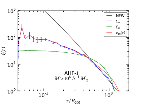
In Fig.  1 we show the comparison between the subhalo 2PCF (green) and the cross CF between subhaloes and the halo centre (blue); in the figure we also show for comparison the number density profile $\rho(r)$ (red) of the subhaloes in the halo Aq-A. The subhaloes are those with $M>10^{6}\,h^{-1}\,{\rm M_{\odot}}$ from the AHF finder, but the comparisons from other finders are similar.

First of all, we observe that the number density profile and the cross CF are similar measurements, since both are measuring the amount of subhaloes as a function of the radial distance to the centre of the halo. To make a fair comparison we have normalized the number density profile a factor of $1/n_{s}$, since this factor relates both magnitudes. The only difference between them is at the edge of the halo, where $\xi_{hs}$ is close to unity, and the factor $-1$ of equation 4 becomes relevant.

On the other hand, we can see that $\xi_{ss}$ is flatter than $\xi_{hs}$. This is expected since $\xi_{ss}$ is measuring the distance between pairs of subhaloes and the probability of having pairs at large distances must be larger that in the case of $\xi_{hs}$, where one of the pairs is always in the centre. We show the shot-noise error bars of the correlation functions in order to show that the statistics of subhaloes is enough to trust their differences. Finally, the black line shows the NFW (Navarro et al., 1996) fit of the dark matter field of the halo (see Table $2$ of Springel et al. 2008). We normalized the number density profile to make our comparison more visible. We can see that the number density profile of subhaloes is very different than the NFW profile of the dark matter, at least for subhaloes in $r/R_{200}<0.4$ (around $100\,h^{-1}\,{\rm kpc}$ for this particular halo). One of the causes of these differences can be an effect of exclusion produced in the inner regions, where the core of the halo dominates, the subhaloes are easily merged, and there are strong tidal stripping effects that can disrupt the subhaloes (and lose mass beyond our sensitivity). Then, although there is a high density, it is difficult to find substructure.

On the other hand, understanding the difference between subhalo and dark matter profiles can be a step forward to galaxy formation. In some halo models of galaxy clustering, such as HOD and CLF models (e.g., Zheng et al. 2007; van den Bosch et al. 2007; Zehavi et al. 2011), it is typically assumed that galaxies follow the dark matter distribution, with a NFW profile and a particular mass-concentration relation (e.g., Macciò et al. 2008). Recent models also account for the fact that the distributions of subhaloes (e.g. Gao et al. 2004; Klypin et al. 2011) and satellite galaxies (e.g. Yang et al. 2005; Wojtak & Mamon 2013) appear to be less concentrated than that of dark matter. On the other hand, SHAM models directly associate galaxies with identified subhaloes. A potential difficulty is the treatment of stripped, disrupted, or ‘orphan’ satellites, in which the subhalo has been stripped and is no longer resolved but the galaxy remains intact. We discuss this further later in the paper.

Figure 1: Comparison between the 2PCF of subhaloes (green), the cross CF between the centre of the halo and the subhaloes (blue) and the number density profile (red) in Aq-A-1 for subhaloes with $M>10^{6}\,h^{-1}\,{\rm M_{\odot}}$ from AHF. The black line shows the NFW dark matter density profile of the halo. The normalization of this profile has been done to compare it better with the other lines. To make a fair comparison between the number density profile and the cross CF, we have normalized the number density profile by a factor $1/n_{s}$. Here $R_{200}=245.76\,h^{-1}\,{\rm kpc}$. The errors of the correlation functions are from Poisson shot-noise.

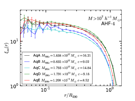
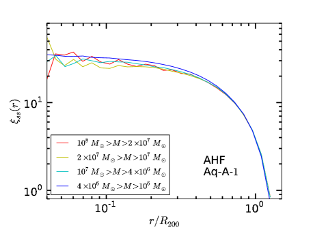
In Fig.  2 we study the difference between haloes by measuring the 2PCF of subhaloes for all the Aquarius haloes at level $4$ of resolution. We show the measurement for the AHF subhaloes, although the other finders show similar results. A mass threshold of $M>10^{7}\ \,h^{-1}\,{\rm M_{\odot}}$ has been applied. We need to increase the mass threshold with respect to Fig. 1 because the resolution in Fig. 2 is lower. In order to compare the haloes, the same normalization has been applied. We have assumed a mean number density of subhaloes according to the number of subhaloes in the Aq-A halo, so $n_{s}=N_{s,\rm AqA}(\rm Mpc/h)^{-3}$. As all the haloes belong to the same cosmology, they should have the same cosmological $n_{s}$. Then, in Fig.  2 we see the contribution of each halo to the 1-halo term of the 2PCF of subhaloes in a large cosmological simulation, with an arbitrary normalization. In this sense, haloes with more subhaloes will tend to contribute more strongly. There are clear differences between haloes that are not due to the lack of statistics, as shown from the shot-noise error bars (for clarity of the figures we will not show these errors in the rest of the figures of the study, but the magnitude of these errors is the same in all the paper). Note that these differences are not caused by our arbitrary normalization of $n_{s}$ in Eq.3. The normalization has to be the same for all haloes, as we are measuring the correlation with respect some global (but unknown) universal mean density of subhaloes (above $M>10^{7}\ \,h^{-1}\,{\rm M_{\odot}}$). If we change the normalization value all correlations will change by the same factor.

For the 2 cases where masses are very similar (C and D) the one with larger concentration has lower amplitude. This is due to the fact that halo Aq-C has much less subhaloes than Aq-D, and then the contribution to the 1-halo term of the 2PCF is smaller. This is an indication that the evolution or other properties of the haloes can produce differences in the clustering although having the same mass. As the Aq-A halo is the only one from where the highest resolutions are available for some of the finders, we will focus on this halo in the rest of the study.

Figure 2: Comparison of the different haloes of the 2PCF of subhaloes for the AHF finder at level $4$ of resolution. The subhaloes have a mass threshold of $M>10^{7}\ \,h^{-1}\,{\rm M_{\odot}}$. Errors are from Poisson shot-noise.

4.2 Density profiles

In Fig. 3 we show the subhalo number density profile of the Aq-A halo for each of the subhalo finders at the 4th level of resolution. In the top panel, the number density profile is restricted to subhaloes with $M>10^{7}\,h^{-1}\,{\rm M_{\odot}}$, while the bottom panel shows the number density profile using a subhalo mass threshold of $M>10^{8}\,h^{-1}\,{\rm M_{\odot}}$. For most of the finders there is good agreement however, especially when the smallest subhaloes are included, we can see a large excess of subhaloes for AdaptaHOP with respect to the rest of the finders. In what follows this finder will often show differences with respect to the others in the comparisons. This is largely because, as discussed elsewhere (Onions et al., 2012; Knebe et al., 2013) this finder do not include a proper unbinding procedure in their subhalo extraction process which can lead to an overdetection of subhaloes as explained in §3.1.

We can also see that the radial range of these number density profiles depends upon the mass threshold. This is largely because the more massive subhaloes are significantly rarer. Although they appear to preferentially reside in the outer part of the halo this is in fact not the case: the number density profile of the more massive haloes is significantly steeper than the low mass subhaloes and they are in fact, as expected due to dynamical friction, more centrally concentrated than the low mass subhaloes.

Figure 3: Comparison of the subhalo number density profile of the Aq-A halo at resolution level $4$ for all the contributing finders. A mass threshold of $M>10^{7}\,h^{-1}\,{\rm M_{\odot}}$ (top) and $M>10^{8}\,h^{-1}\,{\rm M_{\odot}}$ (bottom) has been applied. For Aq-A, $R_{200}=245.70\,h^{-1}\,{\rm kpc}$. The black dashed line represents de NFW fit of the dark matter density profile of the halo with an arbitrary normalization.

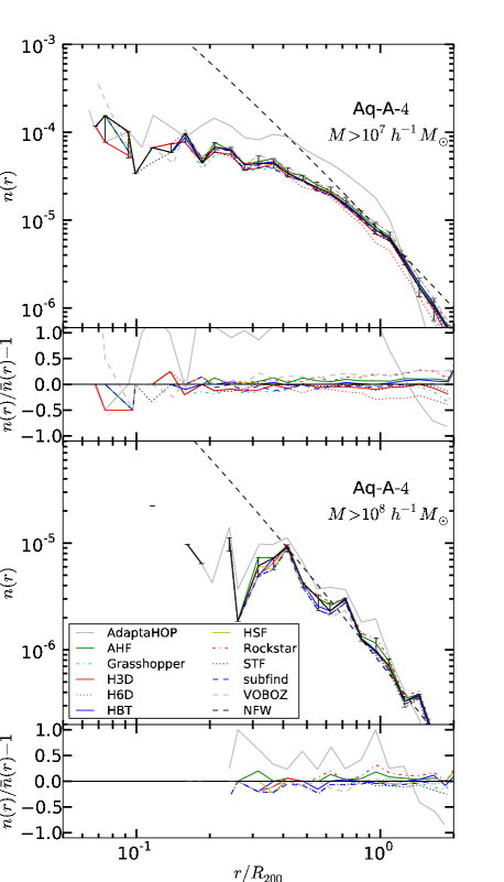
As we can see from Fig. 3 the subhalo number density profile is not only different from the underlying dark matter density profile of the host halo but it also depends on the mass of the subhaloes, being significantly steeper and so more centrally concentrated for higher subhalo masses. These effects could have important consequences when trying to understand the distribution of galaxies in haloes but would need to be investigated with a large ensemble of host haloes spanning a broad range of mass and formation history rather than the small number we have at our disposal here. A study along these lines could be used to improve the models of subhalo statistics from the halo model (Cooray & Sheth, 2002; Sheth & Jain, 2003; Giocoli et al., 2010).

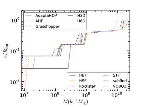
In Fig. 4 we study how stable the different finders are at recovering haloes of different masses as a function of distance from the halo centre. We recover the minimum radial distance where subhaloes below the stated mass first appear. A systematic offset in this figure would indicate a finder that was struggling to find subhaloes close to the halo centre. Due to their rarity more massive subhaloes are found farther from the halo centre than small subhaloes. The agreement between finders for the most massive subhaloes is remarkable but not exactly surprising: such large objects far from the halo centre are easy to spot. The scatter between the finders is larger in the low mass region where the presence or absence of a small object near the halo centre can make a difference.

Figure 4: Minimum radial distance to the halo centre that a subhalo below the stated mass first appears for all the different subhalo finders.

$R_{min}(R/R_{200})$ at different Mass thresholds
	AHF		Rockstar		SUBFIND
Level	$10^{8}\,h^{-1}\,{\rm M_{\odot}}$	$10^{9}\,h^{-1}\,{\rm M_{\odot}}$	$10^{8}\,h^{-1}\,{\rm M_{\odot}}$	$10^{9}\,h^{-1}\,{\rm M_{\odot}}$	$10^{8}\,h^{-1}\,{\rm M_{\odot}}$	$10^{9}\,h^{-1}\,{\rm M_{\odot}}$
1	0.04432	0.33402	0.15591	0.33389	0.08659	0.33395
2	0.07197	0.34480	0.07190	0.37981	0.07193	0.34472
3	0.03406	0.32940	0.00171	0.00171	0.07818	0.32933
4	0.06800	0.37821	0.06789	0.37827	0.11624	0.37815
5	0.13018	0.30310	0.13065	0.30300	0.13067	0.39331

Table 3: Values of $R_{min}$ for subhalo mass thresholds of $10^{8}\,h^{-1}\,{\rm M_{\odot}}$ and $10^{9}\,h^{-1}\,{\rm M_{\odot}}$ as a function of resolution level for AHF, Rockstar and SUBFIND. All the measurements are for the Aq-A halo.

The same trend appears for all the resolution levels, as seen in Table  3. Here we list the different values of $R_{min}$ for two different subhalo mass thresholds ($10^{8}\,h^{-1}\,{\rm M_{\odot}}$ and $10^{9}\,h^{-1}\,{\rm M_{\odot}}$) at all $5$ resolution levels. These measurements are shown for AHF, Rockstar and SUBFIND, the only finders that reach the highest resolution level. First of all, we can see that the agreement between finders for the heaviest subhaloes is very good, with the exception of Rockstar at level $3$, where an exceptional subhalo is found very close to the centre. If we exclude these subhaloes, the Rockstar agrees with the others. However, for the low mass subhaloes the agreement is not so good. This is not surprising because these small substructures can move dramatically within the halo when the extra small scale power is added to the initial power spectrum as the resolution is increased. This issue particularly affects the central regions of the halo which are highly non-linear. However, at a fixed resolution level the finders are trying to extract the same objects. For small masses we must be careful when we measure the distribution of subhaloes in the innermost regions as these structures are easy to miss. For large masses, $R_{min}$ is not only common to all the resolutions but also in all the finders.

The location of subhaloes within a larger halo and the distribution of these subhaloes with mass is a consequence of the interplay of the merging history of the halo, tidal stripping and dynamical friction. This has important implications for SHAM and other subhalo models. Firstly, it is necessary to assess the systematic uncertainties of one’s subhalo finder as a function of resolution and radius (e.g., such that subhaloes in central regions aren’t preferentially lost). Secondly, if one is confident with one’s subhalo finder, it is necessary to account somehow for the subhaloes that have been lost and determine whether ‘orphan’ satellite galaxies have survived (e.g., Hopkins et al. 2010).

4.3 Mass Fractions

In Fig. 5 we show the fractional mass of the host halo that is in subhaloes in the Aq-A halo at resolution level 4 for each of the subhalo finders. The values are shown in terms of mass threshold. We can see that each subhalo finder shows a different mass fraction, and the differences between them are approximately constant in the range between $10^{7}\,h^{-1}\,{\rm M_{\odot}}$ and $10^{9}\,h^{-1}\,{\rm M_{\odot}}$, meaning that the differences are largely due to the size of the biggest subhaloes. We can see that GRASSHOPPER associates a lot of mass with the largest subhalo. This is also an important result from the perspective of SHAM models, as it implies that the dynamical friction time-scales and merger rates inferred from different halo-finding algorithms can vary significantly.

Figure 5: Fractional mass of the host halo in subhaloes for the different finders as a function of the subhalo mass threshold in the Aq-A halo at resolution level 4. We restrict this analysis to within $R_{200}$.

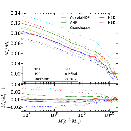
The radial distribution of subhalo mass has already been examined by Onions et al. (2012) who show the cumulative mass fraction of subhaloes as a function of their radial distance from the halo centre. They found good agreement between the finders except for an excess of subhaloes for AdaptaHOP . This work and Fig. 5 shows that most of the finders are apparently consistent in recovering the masses and radial distances of the subhaloes. This is studied in more detail in §4.4.

4.4 Correlation Functions

Figure 6: Comparison between the different finders of the cross CF of subhaloes and the centre of the halo in Aq-A-4 for subhaloes with $M>10^{7}\,h^{-1}\,{\rm M_{\odot}}$ (top left), $v_{\rm max}>12\ {\rm km}~{}{\rm s}^{-1}$ (top right panel), and for top $1000$ subhaloes in mass (bottom left panel) and top $1000$ subhaloes in $v_{\rm max}$ (bottom right panel). In the upper part of these panels the black line and the error bars correspond to the median and the $1\sigma$ percentiles respectively. In the subpanels we show the difference compared to this median. The error bars shown in the subpanels represent the poisson shot-noise of the AHF finder (all the finders are equivalent) centred in the median. For this halo $R_{200}=245.70\,h^{-1}\,{\rm kpc}$.

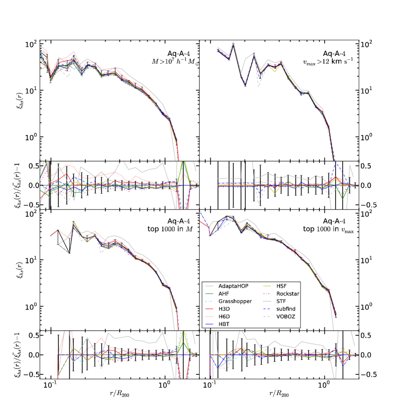
In Fig. 6 we show a comparison of the cross CF of subhaloes using different sample cuts. In all the subpanels we show the normalized differences of the finders with respect to the median, and we show the poisson shot-noise of AHF finder. Since this errors is very similar for all the finders we can assume that this error is a good representation of the shot-noise scatter of these comparisons. In the top left panel we show a comparison of the cross CF of subhaloes with $M_{s}>10^{7}\,h^{-1}\,{\rm M_{\odot}}$ for the different finders, at resolution level 4. There is a good level of agreement between the different finders, apart from an excess in AdaptaHOPand HOT6D. These results are consistent with those of §4.2 and §4.3. On the other hand, we see from the top right panel of Fig. 6 that the agreement is even better if we use a $v_{\rm max}$ threshold instead of a mass threshold. This is because $v_{\rm max}$ is less dependent on the finder than mass, as shown in Fig. 3 and 6 in Onions et al. 2012. This can be explained by the fact that for mass selected subhaloes the agreement between the finders depends strongly on how each finder defines the edge of the subhalo. However the peak of the rotation curve, $v_{\rm max}$, is defined by the central part of the halo (Muldrew et al., 2011), so the differences between the finders in $v_{\rm max}$ are not so strong. In order to make a fair comparison between mass and $v_{\rm max}$ cuts we show in bottom panels the finder comparison by selecting the top $1000$ subhaloes in mass (left) and $v_{\rm max}$ (right). We can see that the agreement between finders is stronger when we use the $v_{\rm max}$ cut, although in both cases there is a clear excess of AdaptaHOP. As the results using density cuts are similar and present the same conclusions than using mass or $v_{\rm max}$ thresholds, we focus on the mass dependence of clustering in the paper and we include a study of the $v_{\rm max}$ dependence in the Appendix A.

Fig. 7 shows the 2PCF of subhaloes within $R_{200}$ and with $M>10^{7}\,h^{-1}\,{\rm M_{\odot}}$ for all the different subhalo finders in Aq-A in resolution level 4. We can see an excess of subhaloes in HOT6D and the fact that the shot-noise errors of the 2PCF are smaller.

4.5 Resolution dependence

In order to see the convergence of the finders with the improving resolution, we used SUBFIND, Rockstar and AHF, since they are the only finders to complete the analysis of all the resolution levels. In Fig. 8 we see how $\xi_{ss}(r)$ depends on the resolution for these $3$ subhalo finders. In order to avoid resolution effects due to small haloes at each level, we exclude all the subhaloes with less than $50$ particles (so each level is resolved down to a different mass threshold according to Table 1). The results for level 4 have already been presented for all finders above. First of all, we can see that levels $4$ and $5$ present distortions at the smallest scales with respect to the rest of the levels. So, a high resolution allows us to find subhaloes with smaller separations between them that we cannot detect at lower resolution. This is also an indication of the presence of subhaloes within subhaloes. Moreover, due to the lower subhalo number the shapes of levels $4$ and $5$ are also more irregular than those of the highest levels. This can give an idea of the scatter of $\xi_{ss}$ at these scales due to the resolution of the simulation. As in the highest resolutions we are including smaller subhaloes, this comparison is also an indication that the smallest subhaloes smooth the shape of $\xi_{ss}$.

Figure 7: Comparison between the different finders for the 2PCF of subhaloes with $M>10^{7}\,h^{-1}\,{\rm M_{\odot}}$ in the Aq-A halo at resolution level 4. Only subhaloes inside $R_{200}$ are considered. The error bars are obtained as in Fig. 6.

Surprisingly, finders appear in better agreement at intermediate resolutions. The discrepancies from level $5$ are due to the poor resolution few subhaloes are detected. In levels $2$ and $3$ the scatter is very low ($\lesssim 5\%$). Given the agreement at this level we can say that the finders AHF, Rockstar and SUBFIND present very small differences between them when $\xi_{ss}$ includes all the subhaloes (with more than $50$ particles). This is an important conclusion, since it means that the definition of subhalo would not affect the measurements of small scale clustering more than a few percent, and then measurements of high precision could be considered reliable. However, in the highest level of resolution the scatter becomes larger again, up to $10$ percent. This discrepancy means that finders, at this level of resolution, have different capabilities of finding small substructure. Rockstar finds more subhaloes with the smallest masses, while SUBFIND tends to be more conservative and finds less subhaloes. The difference in the clustering seen in the last panel of Fig. 8 can be an indication that these subhaloes found by Rockstar are precisely the most clustered ones. These differences are only due to the differences in the algorithms of the finders. In general SUBFIND is one of the most conservative finders, in the sense that less particles tend to be assigned to the subhaloes. Then, for a given mass threshold SUBFIND presents fewer subhaloes. In the centre of the halo the density is higher and the disruption of the subhaloes is stronger. This can make it difficult to find small subhaloes unless a strong dynamical analysis is made. On the other hand, Rockstar is designed to produce accurate dynamical analyses for the structures. This allows the detection of subhaloes which are being disrupted more easily, and also allows two different subhaloes which are crossing but not merging to be distinguished. We must also mention that some of these extra subhaloes in the centre can be artifacts. In the end, Rockstar will find more subhaloes in the most clustered regions, and SUBFIND is designed to be more conservative than the others when claiming a subhalo detection. From Fig. 8 we can see that these differences appear in the highest resolution. It is important to mention that the galaxy distribution within a large halo is affected by the merging history of the haloes and subhaloes that make it, and because of this Rockstar subhaloes may better reflect galaxy clustering at these small scales.

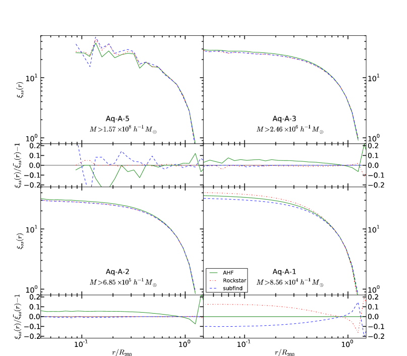
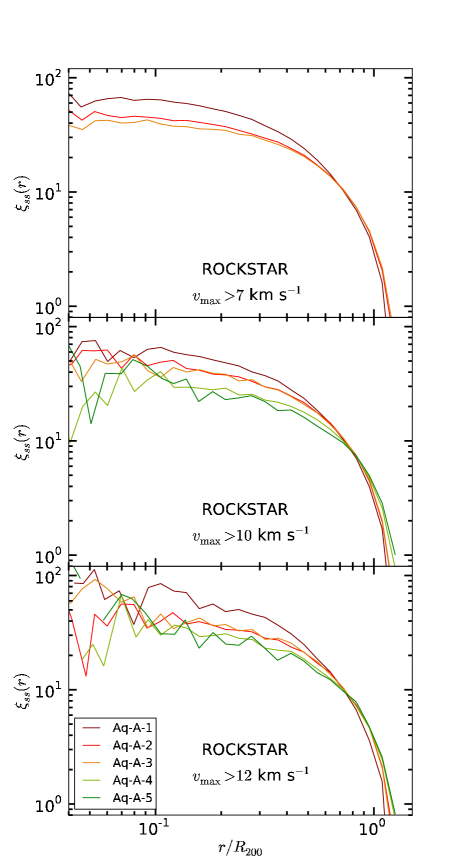
We analyse how $\xi_{ss}(r)$ changes with resolution level in Fig. 9, where we see the resolution dependence of Rockstar with different mass thresholds (for $v_{\rm max}$ thresholds see Fig. 14). The top panel shows $\xi_{ss}(r)$ in resolution levels 4 to 1 for subhaloes with $M>10^{7}\,h^{-1}\,{\rm M_{\odot}}$. We have excluded level $5$ since this mass is below $20$ particles at this level. Although we only show results for Rockstar, the other finders present similar results. The bottom panel shows the same plot for a mass threshold of $M>10^{8}\,h^{-1}\,{\rm M_{\odot}}$. First of all, notice that for bottom panel with the highest mass threshold we cannot see a strong dependence of $\xi_{ss}(r)$ on resolution. However in the top panel, with a lower mass threshold, we can see a clear dependence of clustering on the resolution, showing in the highest level a higher $\xi_{ss}(r)$, so the results in Aq-A-1 halo have not converged yet. In general, Rockstar shows less convergence than the other finders. The resolution dependence in Rockstar is stronger and affects larger subhaloes than for the other finders (AHF and SUBFIND). For these other finders we need to go to smaller subhaloes to see the same effect. As at each level we use the same threshold, the values of the clustering of these subhaloes are only dependent on the resolution. In other words, when the resolution is improved the subhalo clustering changes and an extra term appears in $\xi_{ss}(r)$. The extra term must come from the smallest subhaloes, since the largest ones do not show this term. This could be due to the appearance of small subhaloes included in big structures at the highest resolution level, which would suppose an indication of a 1-subhalo term in the 2PCF.

Figure 8: The subhalo 2PCF of SUBFIND, Rockstar and AHF in Aq-A at resolution levels 5,3,2 & 1 for subhaloes with more than 50 particles.

This effect is important for the smallest subhaloes and it can have implications for galaxy clustering. Although these subhaloes are small, they can originate from larger subhaloes that have lost much of their mass since they were accreted by the host halo. This can be important for some halo abundance matching and other halo models, because the detection of these subhaloes and their present and past properties can complicate the inferred presence and distribution of satellite galaxies in the inner regions of haloes. The differences may be important when comparing halo models of galaxy clustering to observed clustering at small scales (e.g., Wetzel et al. 2009; Watson et al. 2012).

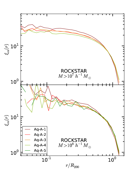
As a consequence of this, the dependence on mass must change with resolution, since the smallest subhaloes change their clustering faster than the largest ones. In order to see this explicitly, in Fig. 10 we show the mass dependence of AHF in mass bins for the highest resolution level 1. We use bins instead of thresholds to see more clearly the mass dependence of clustering. The results for SUBFIND and Rockstar are similar, although not shown. For the other resolution levels the dependence on mass is very weak or non-existent. At level $1$ the smallest subhaloes are the ones with the highest $\xi_{ss}(r)$. This is due to the fact that, from Fig. 9, the smallest subhaloes increase their clustering with resolution faster than the most massive ones do. The effects of Fig. 9 and 10 are stronger if $v_{\rm max}$ dependence is studied instead of mass (see Figs. 14 and 15). At some point, the $\xi_{ss}(r)$ of the smallest subhaloes reaches the $\xi_{ss}(r)$ of the largest ones, and after that the mass (or $v_{\rm max}$) dependence is inverted. As this effect is due to the resolution of the simulation, we can say that at least for resolutions below level $1$ $\xi_{ss}(r)$ is not sensitive to the relation between mass (or $v_{\rm max}$) and clustering. This is due to the fact that low resolutions are not able to detect small subhaloes because they simply don’t contain enough particles. This result is important since there are no large scale simulations nowadays with the resolution of level $1$, and for all these simulations we could be underestimating the clustering of the smallest subhaloes. If the difference is because of the inclusion of the substructure of subhaloes, we can say that one of the effects of including this 1-subhalo term is the inversion of the mass (or $v_{\rm max}$) dependence on clusteringat these scales.

Figure 9: The subhalo 2PCF of Rockstar in Aq-A at 4 different resolution levels for two mass thresholds. In the top panel, the sample corresponds to subhaloes with $M>10^{7}\,h^{-1}\,{\rm M_{\odot}}$. The bottom panel shows subhaloes with $M>10^{8}\,h^{-1}\,{\rm M_{\odot}}$.

Figure 10: 2PCF of subhaloes from AHF for different mass thresholds as indicated in the panel for Aq-A resolution level 1.

5 Halo Model

To describe the 2PCF and cross CF analytically, we follow the extended halo-model formalism developed by Sheth & Jain (2003) and Giocoli et al. (2010). Since real space convolutions are represented by multiplications in Fourier space, we first write the equations of the power spectra and then convert them to real space:

$$\xi(r)=\dfrac{1}{2\pi^{2}}\int k^{3}P(k)\dfrac{\sin(kr)}{kr}\dfrac{\mathrm{d}k}{k}\,.$$ (5)

As in the halo model formalism for the matter power spectrum reconstruction (Scherrer & Bertschinger, 1991; Seljak, 2000; Scoccimarro et al., 2001; Cooray & Sheth, 2002), the subhalo-subhalo power spectrum can be split into a Poisson term $P_{ss,1H}(k)$ that describes the contribution from subhalo pairs within an individual halo (the ‘one-halo term’), plus a large-scale term $P_{ss,2H}(k)$ that describes the contribution from subhaloes in separate haloes (the ‘two-halo term’):

$$P_{ss}(k)=P_{ss,1H}(k)+P_{ss,2H}(k)\,.$$ (6)

Both terms require knowledge of the subhalo spatial density distribution, and the halo and subhalo mass functions. In particular, the second term requires a model for the power spectrum of haloes with different mass $P_{hh}(k|M_{1},M_{2})$ that with good approximation can be expressed as a function of the halo bias $b(M)$ and the linear matter power spectrum $P_{\rm lin}(k)$:

$$P_{hh}(k|M_{1},M_{2})\approx b(M_{1})b(M_{2})P_{\rm lin}(k)\,.$$ (7)

To model the spatial density distribution of subhaloes $n_{s}$ around the center of a halo with mass $M$ and concentration $c=r_{s}/R_{200}$, needed in the reconstruction of both the one-halo and the two-halo term in equation (6), we adopt the analytical fitting function by Gao et al. (2004), motivated by an analysis of results from numerical simulations:

$$f(<r|c)=\dfrac{n_{s}(<x|c)}{N_{tot}(M|c)}=\dfrac{(1+\alpha c)x^{\beta}}{1+\alpha cx^{2}}\,,$$ (8)

where $x$ is the distance from the center in unit of $R_{200}$, $\alpha=0.244$, $\beta=2.75$ and $N_{tot}(M|c)$ represents the total number of subhaloes within $R_{200}$, that we assume to depend both on host halo mass and concentration (De Lucia et al., 2004; van den Bosch et al., 2005; Giocoli et al., 2008, 2010). It has been observed that, at a given redshift, more massive haloes host on average more substructures than less massive ones, because of their lower formation redshift; in addition, at a fixed mass and redshift, more concentrated haloes host fewer structures than less concentrated ones (Gao et al., 2008). To compute the normalized Fourier transform of the subhalo distribution in a spherically symmetric system, we numerically solve the equation:

$$u_{s}(k|c)=\int_{0}^{R_{200}}4\pi r^{2}\dfrac{\sin kr}{kr}f_{s}(r|c)\mathrm{d}r,$$ (9)

where $f_{s}(r|c)$ represents the normalized differential subhalo density distribution around the host halo center, i.e. with the condition that $f_{s}(<R_{200})=1$.

Now we can write the one-halo and the two-halo term of the subhalo-subhalo power spectrum as follows:

$$P_{ss,1H}(k) =\int_{M}\dfrac{n(M)}{\bar{N}_{tot}^{2}}\times$$ (10)

$$\int_{c}N^{2}_{tot}(M|c)\,u^{2}_{s}[k|c(M)]\,p(c|M)\mathrm{d}c\,\mathrm{d}M,$$

$$P_{ss,2H}(k) =P_{lin}(k)\left[\int_{M}\dfrac{n(M)b(M)}{\bar{N}_{tot}}\right.\times$$ (11)

$$\left.\int_{c}N_{tot}(M|c)\,u_{s}[k|c(M)]p(c|M)\mathrm{d}c\,\mathrm{d}M\right]^{2}.$$

where $n(M)$ is the halo mass function, $\bar{N}_{tot}$ the comoving mean number density of satellites in the universe, $p(c|M)$ the log-normal scatter in concentration at fixed halo mass, and we explicitly express the mass dependence of concentration in $u_{s}(k)$.

For the halo-subhalo cross power spectrum we have, respectively:

$$P_{hs,1H}(k) =\int_{M}\dfrac{n(M)}{\bar{N}_{tot}\bar{N}_{h,tot}}\times$$ (12)

$$\int_{c}N_{tot}(M|c)\,u_{s}[k|c(M)]\,p(c|M)\mathrm{d}c\,\mathrm{d}M,$$

and

$$P_{hs,2H}(k) =P_{lin}(k)\int_{M_{1}}\dfrac{n(M_{1})b(M_{1})}{\bar{N}_{tot}}\times$$ (13)

$$\int_{c} N_{tot}(M_{1}|c)\,u_{s}[k|c(M_{1})]p(c|M_{1})\mathrm{d}c\,\mathrm{d}M_{1}\times$$

$$\int_{M_{2}}\dfrac{n(M_{2})b(M_{2})}{\bar{N}_{h,tot}}\mathrm{d}M_{2},$$

where $\bar{N}_{h,tot}$ represents the comoving mean number density of haloes in the Universe. Note that (10) and (12), respectively, can be thought of as contributions from satellite-satellite and center-satellite terms in a halo (Sheth, 2005; Skibba et al., 2006).

Since we are measuring the 2PCF and CF of the subhalo distribution within $R_{200}$ in a single halo, the important terms will be only the Poisson ones $P_{ss,1H}$ and $P_{sh,1H}$; the large-scale terms (11) and (13) appear only when measurements in a simulation can be extended out to larger separations ($r\gg R_{200}$).

In Fig. 11 we compare this halo-model description of the one-halo terms of $\xi_{ss}(r)$ and $\xi_{hs}(r)$ to the measured 2PCF and cross CF of the Aq-A-1 run. For this purpose, we have chosen to compare our analytical predictions to the SUBFIND  catalogue, as the spatial subhalo density distribution model of Gao et al. (2004) has been tuned to a set of simulations in which subhaloes are identified with the same algorithm. For the halo and subhalo mass functions, we have adopted those from Sheth & Tormen (1999) and Giocoli et al. (2010), respectively. We have used the same halo parameters of the A-Aq-1 halo – the integrals on the mass function and on the concentration distribution are restricted around the halo parameters of the halo (see Table 1) – and have adopted an arbitrary normalization, as was done for the measurements in the numerical simulation.

Figure 11: Comparison of the two-point autocorrelation and cross-correlation functions of the extended halo-model formalism and the measurements of the Aq-A-1 run with the subhaloes identified with SUBFIND (similar to Fig. 1). The solid green and blue lines show the 2PCF and cross CF of the simulation, while the red dashed and dotted curves show the halo-model predictions, respectively. In the bottom frame we show the residuals of the measurements with respect to the halo model prediction.

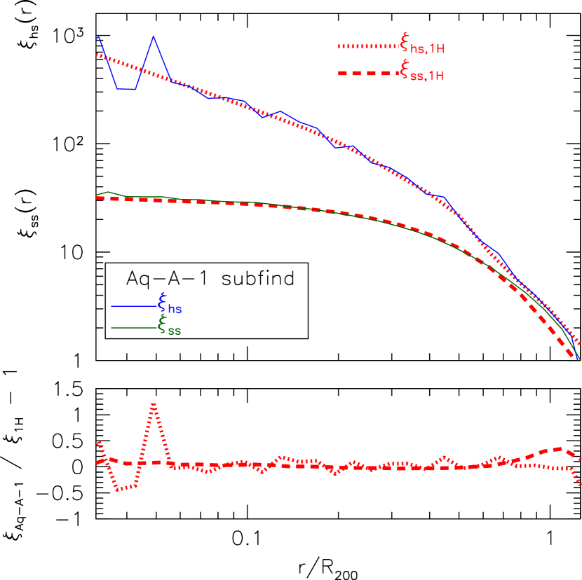
There is clearly very good agreement between the halo model prediction and the simulation, for both the subhalo-subhalo and halo-subhalo clustering signals, over a wide range of scales. This lends support for the model, which provides a good description for the abundance and distribution of subhaloes around a host halo, as calibrated by Gao et al. (2004) for cluster-size haloes and extended in this work to the Aquarius simulation. It also demonstrates that this simulation does not contain an atypical halo, in the sense that its substructures appear to be consistent with the average clustering properties of multiple haloes in other simulations (Gao et al., 2004; Giocoli et al., 2010).

6 Discussion and conclusions

Using a diverse set of subhalo finders, we studied the radial distribution of subhaloes inside Milky Way-like dark matter haloes as simulated within the framework of the Aquarius project. Our interest was focused on the number density profile and two-point correlation functions (2PCF), respectively, investigating any possible variations coming from the utilization of distinct finders as well as the convergence of the results across the different resolution levels of the simulation itself. This work forms part of our on-going ”Subhalo Finder Comparison Project” described in greater detail elsewhere (e.g. Knebe et al., 2013). And following the spirit of the previous comparisons, each code was only allowed to return a list of particle IDs from which a common post-processing pipeline calculated all relevant subhalo properties, including the position. However, this pipeline does not per-se feature an unbinding procedure which was still left to the actual finder in this study.

Our principal conclusions can be summarized as follows:

(i) The number density profile and radial distribution of subhaloes in the Aquarius haloes is different to the underlying dark matter density profile described by the functional form proposed by NFW (Navarro et al., 1996). This is an important result, since in many studies and observations one assumes a NFW profile, also for the subhalo distribution. Even more, a deficit of subhaloes in the central regions of the host actually led to the introduction of so-called ’orphan galaxies’ in order to bring observations into agreement with simulations (Springel et al., 2001; Gao et al., 2004; Guo et al., 2010; Frenk & White, 2012): it can and does happen that a dark matter subhalo dissolves due to tidal forces (and lack of numerical resolution) while orbiting in its host halo (e.g. Gill et al., 2004, for a study of these disrupted subhaloes). However, a galaxy having formed prior to this disruption and residing in it should survive longer than this subhalo. Therefore, it became standard practice to keep the galaxy alive even though its subhalo has disappeared, calling it ’orphan galaxy’.

(ii) The number density profile of subhaloes depends on the mass of the subhalo. For each subhalo mass, we have found a minimum distance from the halo centre that increases with subhalo mass (cf. Fig. 4). This is due to the fact that massive subhaloes are rarer, and then it is difficult to find one of them close to the centre. But we also caution the reader that this result is weakened by the fact that practically every halo finder reduces the subhalo mass when placed closer to its host centre (cf. upper panel of Fig.8 in Knebe et al. (2011) and Fig. 4 in Muldrew et al. (2011)).

(iii) The subhalo finders differ considerably on the fraction of mass in subhaloes with the deviations primarily driven by the most massive subhaloes (cf. Fig. 5). We also confirmed (though not explicitly shown here) that most of the mass in subhaloes is localized outside $0.4R_{200}$, consistent with the previous result that the most massive subhaloes are found far from the halo centre.

(iv) All codes show a remarkable agreement on the cross CF and 2PCF inside the radius $R_{200}$. With the exception of AdaptaHOP finder, in most of the cases the agreement between finders is consistent with Poisson shot-noise errors. For the 2PCF using mass bins, we find $10\%$ agreement between finders for $r>0.1R_{200}$, although the shot-noise error decreases faster with $r$. This reassures us that correlation measurements inside (the virial part of) haloes are not influenced by the choice of the finder at the $10\%$ level of accuracy.

(v) However, we did find that for both the lowest and highest resolution levels there are differences amongst the finders. The former can be attributed to poor resolution, whereas the latter clearly reveals differences in the codes: while the contrast for subhaloes in the very central regions increases some finders still struggle to detect those objects flying past the innermost centre of the host. Further, the highest resolution level shows clear signs of sub-subhaloes yet another possible challenge for halo finders.

(vi) The 2PCF of small subhaloes depends strongly on resolution, with increasing clustering for increasing resolutions. This effect is stronger when a $v_{\rm max}$ threshold is applied and for small subhaloes. For $v_{\rm max}>7\ {\rm km}~{}{\rm s}^{-1}$, the 2PCF increases between $10\%$ and $30\%$ (with a shot-noise uncertainty of $5-10\%$) at the highest resolution. This can be an indication of an extra term of the 2PCF detected in the highest resolution, probably the $1$-subhalo term of the correlations (i.e. the existence of sub-subhaloes). As this effect is stronger for the smallest subhaloes, the mass dependence of clustering depends on the resolution, too. In particular, we see that at level $1$ there is an anti-correlation between clustering and mass. The importance of this result resides in the fact that, as there are no large scale simulations with this resolution to-date, the clustering of the smallest subhaloes in these simulation can be systematically underestimated.

(vii) We confirm aforementioned findings when using $v_{\rm max}$ as opposed to mass cuts (cf. Appendix A), albeit a stronger dependence on $v_{\rm max}$. When a $v_{\rm max}$ cut is applied, the difference between finders is smaller than the $5\%$ level for $r>0.2R_{200}$, an agreement consistent with the Poisson shot-noise. As $v_{max}$ retains more information about the past of the subhaloes and provides a more suitable measure when comparing to observations, this result will have more importance for the implications in galaxy formation.

All these results certainly contribute to the understanding of the substructure distribution within dark matter haloes and how much their distribution depends on the finder algorithm and the resolution of the simulation. Moreover, substructure clustering plays an important role for galaxy formation models, because satellite galaxies are expected to follow the subhalo gravitational potentials. Methods such as Sub-Halo Abundance Matching (SHAM) often make this assumption, and Semi-Analytical Models (SAM) model baryonic processes according to the properties of the subhaloes and their merger trees. In these cases, the properties of the subhaloes affect inferred properties of the galaxy population, and a correct definition/identification of subhaloes is crucial. For a given model, using different subhalo finders can produce different galaxy distributions and galaxy-subhalo relations. These differences make it difficult to compare galaxy formation models and their predictions if their assumptions about subhalo definition and identification are treated differently.

Also, HOD models populate galaxies in simulations to infer halo properties from observations, usually a NFW profile of the galaxies in haloes is assumed. But if galaxies follow the subhalo distribution instead of the dark matter field, then the measurement of the subhaloes can also be used in the HOD models to improve the radial distribution of galaxies in haloes.

Improving the resolution of the simulation is also crucial, since we have seen that many subhaloes are lost in the lowest resolution simulations, and they have important consequences for the resulting subhalo clustering. Most of these lost subhaloes are rather small and live in the densest regions of their host, but in these cases they could have been more massive and experienced severe tidal stripping, respectively. If one uses abundance matching to populate galaxies in simulations when the resolution is insufficient, if one is using present subhalo mass or $v_{\mathrm{max}}$ (or also these quantities at the time of accretion), one could be missing an important fraction of galaxies in the centre of the haloes, and workers in the field try to circumvent this by introducing aforementioned orphan galaxies (Springel et al., 2001; Gao et al., 2004; Guo et al., 2010; Frenk & White, 2012). It is therefore important to consistently track haloes and subhaloes when associating them with galaxy populations.

As already highlighted previously (Onions et al., 2013), the (non-)removal of unbound particles will leave an impact on subhalo properties, too – something again confirmed in this work: we have found that AdaptaHOP  show important differences to the rest of the finders, since it does not include a (faithful) removal of unbound particles. AdaptaHOP does not eliminate the background particles from the host – unbound to the subhalo – which produces an overestimation of the number of small subhaloes, especially in the central parts of the halo. This effect clearly leaves an imprint in the number density profile and correlation functions.

The implications of our results also extend to the interpretation of ongoing and upcoming galaxy surveys measuring a fair fraction of the observable Universe (just to name a few, BOSS, PAU, WiggleZ, eBOSS, BigBOSS, DESpec, PanSTARRS, DES, HSC, Euclid, WFIRST, etc.). For their interpretation of the 2-point galaxy correlation function (or alternatively the power spectrum) is commonly used and hence needs to be determined to unprecedented accuracy (e.g. Smith et al., 2012). As we have just seen, the 1-halo and in particular the 1-subhalo term is sensitive to the applied halo finder. Further work and analysis in high resolution cosmological simulations are needed to better understand this.

But all our results have to be taken with a grain of salt: as one single halo does not represent a homogeneous distribution, we must be careful with the definition and interpretation of the 2PCF. We use a theoretical normalization where we assume an infinite and completely homogeneous random field. The results converge to the random sample normalization when the volume of the random sample is large enough. We need to assume an arbitrary mean density of subhaloes, since we cannot measure the abundance of subhaloes expected for a large simulation because there are no large simulations with the resolution of these Aquarius haloes. This measurement of the 2PCF must be understood as the contribution that the halo would give to the $1$-halo term of the 2PCF of a large and homogeneous simulation, since it reflects the number of pairs of subhaloes found inside the halo, with an arbitrary amplitude due to the unknown mean number density of subhaloes.

Appendix A $v_{\rm max}$ dependence

Figure 12: Comparison between the different finders of the 2PCF of subhaloes with $v_{\rm max}>12\ {\rm km}~{}{\rm s}^{-1}$ in the Aq-A halo at level 4 of resolution. The black line and the error bars in the upper part correspond to the median and the $1\sigma$ percentiles respectively, while in the bottom subplot the error bars represent the Poisson shot-noise of the AHF finder (the other finders are equivalent).

Figure 13: The subhalo 2PCF of SUBFIND, Rockstar and AHF in Aq-A at different resolution levels and $v_{\rm max}>10\ {\rm km}~{}{\rm s}^{-1}$ threshold.

Figure 14: The subhalo 2PCF of Rockstar in Aq-A as a function of the resolution levels for $3$ $v_{\rm max}$ thresholds. In the top panel, the sample corresponds to subhaloes with $v_{\rm max}>7\ {\rm km}~{}{\rm s}^{-1}$. In the middle the threshold used is $v_{\rm max}>10\ {\rm km}~{}{\rm s}^{-1}$. Finally, in the bottom panel a threshold of $v_{\rm max}>12\ {\rm km}~{}{\rm s}^{-1}$ has been used.

Figure 15: 2PCF of AHF at different $v_{\rm max}$ thresholds, at levels $1$ (bottom) and $3$ (top).

In this Appendix we explore the same study as in §4 but using $v_{\rm max}$ instead of mass as the subhalo property studied.

In Fig. 12 we see $\xi_{ss}(r)$ for subhaloes with $v_{\rm max}>12\ {\rm km}~{}{\rm s}^{-1}$. However, the agreement is much better for $v_{\rm max}$ thresholds than for mass threshold. This is constant in all the study. We can see in particular that the differences between finders are consistent with the shot-noise errors due to their statistics.

In Fig. 13 we compare the finders AHF  Rockstar and SUBFIND in several resolution levels with the $v_{\rm max}$ threshold $v_{\rm max}>10\ {\rm km}~{}{\rm s}^{-1}$. We do not show level $4$ since it is shown in Fig. 12. First of all, we can see a strong scatter at levels $4$ and $5$ in scales lower than $0.1R_{200}$. This, as in the case of mass thresholds, can be understood from the difficulty of finding subhaloes with small separations at these levels of resolution. Then, these resolutions are not sensitive to the 2PCF of subhaloes at these scales. On the other hand, at larger distances the agreement of the finders at these levels as well as at levels $2$ and $3$ is remarkable. However, the differences become stronger at level $2$ and much larger at level $1$ of resolution. In particular, in level $1$ Rockstar shows a large difference between the other finders. Although the results are equivalent to Fig. 8 where we have used a mass threshold, we find a strong disagreement between ROCKSTAR and the other finders when the $v_{\rm max}$ threshold is applied at level $1$. This is an indication that the extra subhaloes found by Rockstar are precisely those with more clustering as $v_{\rm max}$ is more sensitive to the clustering of these subhaloes than mass.

As we see, $\xi_{ss}(r)$ changes with resolution also for $v_{\rm max}$ thresholds. We can see these changes more explicitly in Fig. 14, where we show $\xi_{ss}(r)$ for Rockstar finder as a function of the resolution using $3$ different $v_{\rm max}$ thresholds ($v_{\rm max}>7\ {\rm km}~{}{\rm s}^{-1}$ on top, $v_{\rm max}>10\ {\rm km}~{}{\rm s}^{-1}$ in the middle and $v_{\rm max}>12\ {\rm km}~{}{\rm s}^{-1}$ in the bottom panel). We only show one finder, but the results are equivalent for the others. For each threshold we only show the levels of resolution that are consistent with this threshold. First of all, we can see that the regularity in the shapes of $\xi_{ss}(r)$ is improved for higher resolutions, meaning that this irregularity is purely due to resolution effects. Secondly, we note that the clustering is higher for higher resolutions in all the thresholds used. We can see this effect clearer using $v_{\rm max}$ thresholds instead of mass thresholds because $v_{\rm max}$ is more strongly related to clustering than mass. As for mass thresholds, Rockstar shows a larger effect than the other finders. Then, in Fig. 14 we can see that an extra term appears in $\xi_{ss}(r)$ when we improve the resolution. This means, again, that simulations with lower resolutions are not able to appreciate this extra term. Subhaloes with low $v_{\rm max}$ increase faster their clustering with resolution than subhaloes with large $v_{\rm max}$, as we will see in Fig. 15. This might be an indication of the sub-substructure detected only in the highest resolutions, as discussed in §4.5.

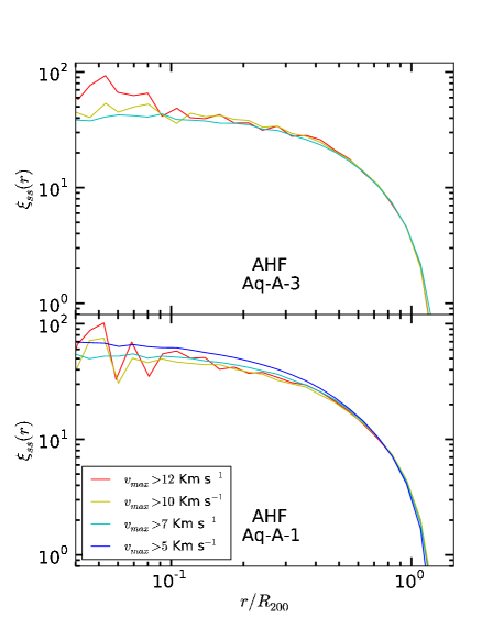
Finally, we analyse the $v_{\rm max}$ dependence of subhalo clustering in Fig. 15. Fig. 15 shows the clustering dependence on $v_{\rm max}$ of AHF finder at levels $1$ (bottom) and $3$ (top). Although the interpretation in the smallest scales is complicated due to the low statistics, the results at larger scales are clear. At level $1$, we see that the lower the threshold, the higher the clustering. However, at level $3$ the relation is the opposite than in level $1$. This result shows that the smallest subhaloes increase their clustering with resolution faster that the largest ones do. The change on clustering is higher if the subhaloes are smaller, and they change up to the point of inverting the relation between clustering and $v_{\rm max}$ from level $3$ to $1$. As the relation between $v_{\rm max}$ and clustering is stronger than mass, the change in the $v_{\rm max}$ dependence is stronger an easier to see that the change on the mass dependence shown in Fig. 10. Again, the appearance of an extra term on the 2PCF of the smallest subhaloes can be an indication of the detection of the $1$-subhalo term of the 2PCF. The fact that this effect also happens for $v_{\rm max}$ threshold is important, since $v_{\rm max}$ is expected to retain more information about the history and past of the subhaloes than mass. The distribution of subhaloes as a function of $v_{\rm max}$ is important for methods of galaxy formation such as SHAM, where subhalo $v_{\rm max}$ has been shown to be a better tracer of galaxies than subhalo mass (Reddick et al., 2013; Hearin et al., 2013). The conclusions made from the mass dependence of this 1-subhalo term about the implications on SHAM are more important when $v_{\rm max}$ is taken into account, not only because $v_{\rm max}$ reflects more galaxy clustering on SHAM galaxies, but also because this effect is even stronger.

References

- Ascasibar (2010) Ascasibar Y., 2010, Computer Physics Communications, 181, 1438
- Ascasibar & Binney (2005) Ascasibar Y., Binney J., 2005, MNRAS, 356, 872
- Avila-Reese et al. (2005) Avila-Reese V., Colín P., Gottlöber S., Firmani C., Maulbetsch C., 2005, ApJ, 634, 51
- Behroozi et al. (2010) Behroozi P. S., Conroy C., Wechsler R. H., 2010, ApJ, 717, 379
- Behroozi et al. (2013) Behroozi P. S., Wechsler R. H., Wu H.-Y., 2013, ApJ, 762, 109
- Benson et al. (2000) Benson A. J., Cole S., Frenk C. S., Baugh C. M., Lacey C. G., 2000, MNRAS, 311, 793
- Berlind & Weinberg (2002) Berlind A. A., Weinberg D. H., 2002, ApJ, 575, 587
- Conroy et al. (2006) Conroy C., Wechsler R. H., Kravtsov A. V., 2006, ApJ, 647, 201
- Cooray (2006) Cooray A., 2006, MNRAS, 365, 842
- Cooray & Sheth (2002) Cooray A., Sheth R., 2002, PhysRep, 372, 1
- De Lucia et al. (2004) De Lucia G., Kauffmann G., Springel V., White S. D. M., Lanzoni B., Stoehr F., Tormen G., Yoshida N., 2004, MNRAS, 348, 333
- Duffy et al. (2008) Duffy A. R., Schaye J., Kay S. T., Dalla Vecchia C., 2008, MNRAS, 390, L64
- Elahi et al. (2013) Elahi P. J., Han J., Lux H., Ascasibar Y., Behroozi P., Knebe A., Muldrew S. I., Onions J., Pearce F., 2013, MNRAS, 433, 1537
- Elahi et al. (2011) Elahi P. J., Thacker R. J., Widrow L. M., 2011, MNRAS, 418, 320
- Frenk & White (2012) Frenk C. S., White S. D. M., 2012, Annalen der Physik, 524, 507
- Gao et al. (2004) Gao L., De Lucia G., White S. D. M., Jenkins A., 2004, MNRAS, 352, L1
- Gao et al. (2008) Gao L., Navarro J. F., Cole S., Frenk C. S., White S. D. M., Springel V., Jenkins A., Neto A. F., 2008, MNRAS, 387, 536
- Gao et al. (2004) Gao L., White S. D. M., Jenkins A., Stoehr F., Springel V., 2004, MNRAS, 355, 819
- Gill et al. (2004) Gill S. P. D., Knebe A., Gibson B. K., 2004, MNRAS, 351, 399
- Gill et al. (2004) Gill S. P. D., Knebe A., Gibson B. K., Dopita M. A., 2004, MNRAS, 351, 410
- Giocoli et al. (2010) Giocoli C., Bartelmann M., Sheth R. K., Cacciato M., 2010, MNRAS, 408, 300
- Giocoli et al. (2012) Giocoli C., Tormen G., Sheth R. K., 2012, MNRAS, 422, 185
- Giocoli et al. (2010) Giocoli C., Tormen G., Sheth R. K., van den Bosch F. C., 2010, MNRAS, 404, 502
- Giocoli et al. (2008) Giocoli C., Tormen G., van den Bosch F. C., 2008, MNRAS, 386, 2135
- Guo et al. (2010) Guo Q., White S., Li C., Boylan-Kolchin M., 2010, MNRAS, 404, 1111
- Han et al. (2011) Han J., Jing Y., Wang H., Wang W., 2011, in Galaxy Formation Resolving Subhalos’ Lives with the Hierarchical Bound-Tracing Algorithm. p. 175P
- Hearin et al. (2013) Hearin A. P., Zentner A. R., Berlind A. A., Newman J. A., 2013, MNRAS, 433, 659
- Hopkins et al. (2010) Hopkins P. F., Croton D., Bundy K., Khochfar S., van den Bosch F., Somerville R. S., Wetzel A., Keres D., Hernquist L., Stewart K., Younger J. D., Genel S., Ma C.-P., 2010, ApJ, 724, 915
- Jing et al. (1998) Jing Y. P., Mo H. J., Boerner G., 1998, ApJ, 494, 1
- Klypin et al. (2011) Klypin A. A., Trujillo-Gomez S., Primack J., 2011, ApJ, 740, 102
- Knebe et al. (2011) Knebe A., Knollmann S. R., Muldrew S. I., Pearce F. R., Aragon-Calvo M. A., Ascasibar Y., Behroozi P. S., Ceverino D., et al. 2011, MNRAS, 415, 2293
- Knebe et al. (2013) Knebe A., Pearce F. R., Lux H., Ascasibar Y., Behroozi P., Casado J., Corbett Moran C., Diemand J., et al. 2013, ArXiv e-prints
- Knollmann & Knebe (2009) Knollmann S. R., Knebe A., 2009, ApJS, 182, 608
- Landy & Szalay (1993) Landy S. D., Szalay A. S., 1993, ApJ, 412, 64
- Macciò et al. (2008) Macciò A. V., Dutton A. A., van den Bosch F. C., 2008, MNRAS, 391, 1940
- Macciò et al. (2007) Macciò A. V., Dutton A. A., van den Bosch F. C., Moore B., Potter D., Stadel J., 2007, MNRAS, 378, 55
- Maciejewski et al. (2009) Maciejewski M., Colombi S., Springel V., Alard C., Bouchet F. R., 2009, MNRAS, 396, 1329
- Mo & White (1996) Mo H. J., White S. D. M., 1996, MNRAS, 282, 347
- Moore et al. (1999) Moore B., Quinn T., Governato F., Stadel J., Lake G., 1999, MNRAS, 310, 1147
- Muldrew et al. (2011) Muldrew S. I., Pearce F. R., Power C., 2011, MNRAS, 410, 2617
- Navarro et al. (1996) Navarro J. F., Frenk C. S., White S. D. M., 1996, ApJ, 462, 563
- Navarro et al. (1997) Navarro J. F., Frenk C. S., White S. D. M., 1997, ApJ, 490, 493
- Neistein et al. (2010) Neistein E., Macciò A. V., Dekel A., 2010, MNRAS, 403, 984
- Neto et al. (2007) Neto A. F., Gao L., Bett P., Cole S., Navarro J. F., Frenk C. S., White S. D. M., Springel V., Jenkins A., 2007, MNRAS, 381, 1450
- Neyrinck et al. (2005) Neyrinck M. C., Gnedin N. Y., Hamilton A. J. S., 2005, MNRAS, 356, 1222
- Onions et al. (2013) Onions J., Ascasibar Y., Behroozi P., Casado J., Elahi P., Han J., Knebe A., Lux H., Merchán M. E., Muldrew S. I., Neyrinck M., Old L., Pearce F. R., Potter D., Ruiz A. N., Sgró M. A., Tweed D., Yue T., 2013, MNRAS, 429, 2739
- Onions et al. (2012) Onions J., Knebe A., Pearce F. R., Muldrew S. I., Lux H., Knollmann S. R., Ascasibar Y., Behroozi P., et al. 2012, MNRAS, 423, 1200
- Peacock & Smith (2000) Peacock J. A., Smith R. E., 2000, MNRAS, 318, 1144
- Reddick et al. (2013) Reddick R. M., Wechsler R. H., Tinker J. L., Behroozi P. S., 2013, ApJ, 771, 30
- Scherrer & Bertschinger (1991) Scherrer R. J., Bertschinger E., 1991, ApJ, 381, 349
- Scoccimarro et al. (2001) Scoccimarro R., Sheth R. K., Hui L., Jain B., 2001, ApJ, 546, 20
- Seljak (2000) Seljak U., 2000, MNRAS, 318, 203
- Sheth (2005) Sheth R. K., 2005, MNRAS, 364, 796
- Sheth et al. (2001) Sheth R. K., Diaferio A., Hui L., Scoccimarro R., 2001, MNRAS, 326, 463
- Sheth & Jain (2003) Sheth R. K., Jain B., 2003, MNRAS, 345, 529
- Sheth & Tormen (1999) Sheth R. K., Tormen G., 1999, MNRAS, 308, 119
- Skibba et al. (2006) Skibba R., Sheth R. K., Connolly A. J., Scranton R., 2006, MNRAS, 369, 68
- Skibba & Macciò (2011) Skibba R. A., Macciò A. V., 2011, MNRAS, 416, 2388
- Smith et al. (2012) Smith R. E., Reed D. S., Potter D., Marian L., Crocce M., Moore B., 2012, ArXiv e-prints
- Springel et al. (2008) Springel V., Wang J., Vogelsberger M., Ludlow A., Jenkins A., Helmi A., Navarro J. F., Frenk C. S., White S. D. M., 2008, MNRAS, 391, 1685
- Springel et al. (2005) Springel V., White S. D. M., Jenkins A., Frenk C. S., Yoshida N., Gao L., Navarro J., Thacker R., et al. 2005, Nature, 435, 629
- Springel et al. (2001) Springel V., White S. D. M., Tormen G., Kauffmann G., 2001, MNRAS, 328, 726
- Srisawat et al. (2013) Srisawat C., Knebe A., Pearce F. R., Schneider A., Thomas P. A., Behroozi P., Dolag K., Elahi P. J., Han J., Helly J., Jing Y., Jung I., Lee J., Mao Y. Y., Onions J., Rodriguez-Gomez V., Tweed D., Yi S. K., 2013, ArXiv e-prints
- Stadel (2001) Stadel J. G., 2001, PhD thesis, University of Washington
- Tinker et al. (2008) Tinker J., Kravtsov A. V., Klypin A., Abazajian K., Warren M., Yepes G., Gottlöber S., Holz D. E., 2008, ApJ, 688, 709
- Tinker et al. (2010) Tinker J. L., Robertson B. E., Kravtsov A. V., Klypin A., Warren M. S., Yepes G., Gottlöber S., 2010, ApJ, 724, 878
- Tormen et al. (2004) Tormen G., Moscardini L., Yoshida N., 2004, MNRAS, 350, 1397
- Trujillo-Gomez et al. (2011) Trujillo-Gomez S., Klypin A., Primack J., Romanowsky A. J., 2011, ApJ, 742, 16
- Tweed et al. (2009) Tweed D., Devriendt J., Blaizot J., Colombi S., Slyz A., 2009, A&A, 506, 647
- van den Bosch et al. (2005) van den Bosch F. C., Tormen G., Giocoli C., 2005, MNRAS, 359, 1029
- van den Bosch et al. (2007) van den Bosch F. C., Yang X., Mo H. J., Weinmann S. M., Macciò A. V., More S., Cacciato M., Skibba R., Kang X., 2007, MNRAS, 376, 841
- Warren et al. (2006) Warren M. S., Abazajian K., Holz D. E., Teodoro L., 2006, ApJ, 646, 881
- Watson et al. (2012) Watson D. F., Berlind A. A., McBride C. K., Hogg D. W., Jiang T., 2012, ApJ, 749, 83
- Wechsler et al. (2002) Wechsler R. H., Bullock J. S., Primack J. R., Kravtsov A. V., Dekel A., 2002, ApJ, 568, 52
- Wetzel et al. (2009) Wetzel A. R., Cohn J. D., White M., 2009, MNRAS, 394, 2182
- White & Rees (1978) White S. D. M., Rees M. J., 1978, MNRAS, 183, 341
- Wojtak & Mamon (2013) Wojtak R., Mamon G. A., 2013, MNRAS, 428, 2407
- Wong & Taylor (2012) Wong A. W. C., Taylor J. E., 2012, ApJ, 757, 102
- Wu et al. (2013) Wu H.-Y., Hahn O., Wechsler R. H., Behroozi P. S., Mao Y.-Y., 2013, ApJ, 767, 23
- Yang et al. (2003) Yang X., Mo H. J., van den Bosch F. C., 2003, MNRAS, 339, 1057
- Yang et al. (2005) Yang X., Mo H. J., van den Bosch F. C., Weinmann S. M., Li C., Jing Y. P., 2005, MNRAS, 362, 711
- Zehavi et al. (2011) Zehavi I., Zheng Z., Weinberg D. H., Blanton M. R., Bahcall N. A., Berlind A. A., Brinkmann J., Frieman J. A., et al. 2011, ApJ, 736, 59
- Zentner et al. (2005) Zentner A. R., Kravtsov A. V., Gnedin O. Y., Klypin A. A., 2005, ApJ, 629, 219
- Zheng et al. (2007) Zheng Z., Coil A. L., Zehavi I., 2007, ApJ, 667, 760
Appendix A dependence