General dissipative coefficient in warm Intermediate and logamediate inflation

Abstract

We study a general form for the dissipative coefficient $\Gamma(T,\phi)=C_{\phi}\,T^{m}/\phi^{m-1}$ in the context of warm intermediate and logamediate inflationary universe models. We analyze these models in the weak and strong dissipative regimes. In the slow-roll approximation, we describe in great detail the characteristics of these models. In both regimes, we use recent data from the WMAP nine-year data and Planck data to constrain the parameters appearing in our models.

I Introduction

It is well known that the inflationary universe model provides an interesting approach for solving some of the problems of the standard big bang model, such as the flatness, the horizon etc.R1 ; R102 ; R103 ; R104 ; R105 ; R106 . One of the achievements of the inflation scenario is that it scenario can offer an elegant mechanism to explain the large-scale structure R2 ; R202 ; R203 ; R204 ; R205 and the observed anisotropy of the cosmic microwave background (CMB) radiationastro ; astro2 ; astro202 ; Planck .

On the other hand, the warm inflation scenario differs from cold inflation in that there is no separate reheating period in the former; rather, radiation production occurs at the same time as inflationary expansion due to the decay of the inflaton field into radiation and particles during the slow-roll phase.warm . In this form, the universe ceases inflating and smoothly enters a radiation-dominated big bang scenario warm ; taylorberera ; taylorberera02 ; taylorberera03 ; taylorberera04 ; taylorberera05 ; taylorberera06 ; taylorberera07 ; taylorberera08 ; taylorberera09 . In the inflationary regime, the dissipative effects are important and originate from a friction term which describes the physical processes of the scalar field dissipating into a thermal bath. Also, during warm inflation the thermal fluctuations represent a dominant role in producing the initial density fluctuations necessary for large-scale Structure (LSS) formation. Here, these density fluctuations arise from thermal rather than quantum fluctuations 62526 ; 6252602 ; 6252603 ; 6252604 ; 1126 .

In the context of the dissipation coefficient $\Gamma$, the particular scenario of low-temperature regimes was presented in Refs.26 ; 28 ; 2802 . There, the value of $\Gamma$ was considered in supersymmetric models which have an inflaton together with multiplets of heavy and light fields. Different choices of $m$ have been adopted or, equivalently, different expressions for the dissipation coefficient have been analyzed in Refs.Zhang:2009ge ; BasteroGil:2011xd ; BasteroGil:2012cm . In this form, following Refs.Zhang:2009ge ; BasteroGil:2011xd , we consider a general form of the dissipative coefficient, given by

$$\Gamma=C_{\phi}\,\frac{T^{m}}{\phi^{m-1}},$$ (1)

where $m$ is an integer and $C_{\phi}$ is associated to the dissipative microscopic dynamics. In particular, for the case $m=3$, the value of $C_{\phi}$ corresponds to $C_{\phi}=0.64\,h^{4}\,\mathcal{N}$, in which ${\mathcal{N}}={\mathcal{N}}_{\chi}{\mathcal{N}}_{decay}^{2}$, where $\mathcal{N}_{\chi}$ is the multiplicity of the $X$ superfield and ${\mathcal{N}}_{decay}$ is the number of decay channels available in $X$’s decay26 ; 27 (see also Refs.Berera:2008ar ; BasteroGil:2010pb ). The dissipation coefficient $\Gamma$ for $m=1$ is given by $\Gamma\propto\,T$ and it represents the high-temperature supersymmetry (SUSY) case; when $m=0$ the dissipation coefficient is $\Gamma\propto\phi$ and it corresponds to an exponentially decaying propagator in the SUSY case; and when $m=-1$ then $\Gamma\propto\phi^{2}/T$, and it corresponds to the non-SUSY case. In particular, the case $m=3$, i.e., $\Gamma\propto T^{3}/{\phi^{2}}$ was considered for the warm intermediate model in Ref.delCampo:2009xi and for the warm logamediate model in Ref.Herrera:2012zz . In the following, we will study the warm intermediate and logamediate inflationary models for the values of $m=1$, $m=0$, and $m=-1$.

On the other hand, the most interesting exact solutions in the inflationary universe is can be found by using an exponential potential, which is often called a power-law inflation since the scale factor has a power-law-type evolution, i.e., $a(t)\sim t^{p}$, in which $p>1$power . Also, an exact solution can be obtained in the de Sitter inflationary universe, where a constant scalar potential is considered; see Ref.R1 . However, exact solutions can also be obtained for the scenario of intermediate inflation Barrow1 . In this universe model the scale factor $a(t)$ growths as

$$a(t)=\exp[\,A\,t^{f}],$$ (2)

where $A$ and $f$ are two constants; $A>0$ and $0<f<1$ Barrow1 . This expansion type is slower than de Sitter inflation, but faster than power-law inflation; this is why it is known as ”intermediate”. Nevertheless, a generalized model of the expansion of the universe is logamediate inflation R12 . In this model, the scale factor $a(t)$ increases as

$$a(t)=\exp[\,A\,(\ln t)^{\lambda}],$$ (3)

where $\lambda$ and $A$ are dimensionless constant parameters such that $\lambda>1$ and $A>0$; see Ref.R12 . Note that for special the case in which $\lambda=1$ and $A=p$, the logamediate inflation model becomes a power-law inflation model power .

Intermediate and logamediate models were originally developed as an exact solution, but they may be best formulated from the slow-roll approximation. During the slow-roll approximation, it is possible to find a spectral index $n_{s}\sim 1$. In particular, in the model of intermediate inflation the value $n_{s}=1$ that corresponds to the Harrizon-Zel’dovich spectrum is found for the special value $f=2/3$ Barrow2 , but this value is not suported by the current observational dataastro ; astro2 ; Planck . Also, an important observational quantity in both models, is that the tensor-to-scalar ratio $r$, which is significantly $r\neq 0$ratior ; Barrow3 .

The main goal of the present work is to analyze the possible realization of an expanding intermediate and logamediate scale factor within the framework of a warm inflationary universe model, and how warm intermediate and logamediate inflation works with a generalized form of the dissipative coefficient. We will study these models for two regimes: the weak and the strong dissipative scenarios.

The paper is organized as follows. The next section presents the basic equations for warm inflation. In Secs. III and IV, we discuss the weak and strong dissipative regimes in the intermediate and logamediate scenarios. In both sections, we give explicit expressions for the dissipative coefficient, the scalar potential, the scalar power spectrum and the tensor-to-scalar ratio for these models. The nine-year WMAP data and Planck data are used to constrain the parameters in our models. In Sec. V, we analyze the interpolation between the weak and strong decays. Finally, Sec. VI summarizes and discuses our finding. We use units in which $c=\hbar=1$.

II Warm Inflation: Basic equations

We consider a spatially flat Friedmann equation, given by

$$H^{2}=\frac{\kappa}{3}\,\rho=\frac{\kappa}{3}\,[\rho_{\phi}+\rho_{\gamma}],$$ (4)

where $H$ denotes the Hubble parameter given by $H=\dot{a}/a$, $a$ is the scale factor, and the constant $\kappa=8\pi G=8\pi/m_{p}^{2}$, where $m_{p}$ denotes the Planck mass. In warm inflation, the universe is filled with a self-interacting scalar field with energy density $\rho_{\phi}$ and a radiation field with energy density $\rho_{\gamma}$. Here, the total energy density $\rho$ is given by $\rho=\rho_{\phi}+\rho_{\gamma}$.

In the following, we will consider that the energy density related to the scalar field is given by $\rho_{\phi}=\dot{\phi}^{2}/2-V(\phi)$ and the pressure is $P_{\phi}=\dot{\phi}^{2}/2+V(\phi)$, where $V(\phi)$ corresponds to the effective potential. Dots mean derivatives with respect to time.

The dynamical equations for $\rho_{\phi}$ and $\rho_{\gamma}$ in warm inflation are described bywarm

$$\dot{\rho_{\phi}}+3\,H\,(\rho_{\phi}+P_{\phi})=-\Gamma\;\;\dot{\phi}^{2},$$ (5)

and

$$\dot{\rho}_{\gamma}+4H\rho_{\gamma}=\Gamma\dot{\phi}^{2},$$ (6)

where $\Gamma>0$ is the dissipation coefficient and it is responsible for the decay of the scalar field into radiation during the inflationary scenario. The dissipation coefficient $\Gamma$ can be considered to be a function of the temperature of the thermal bath $\Gamma(T)$, the scalar field $\Gamma(\phi)$, both $\Gamma(T,\phi)$, or a constantwarm .

During warm inflation $\rho_{\phi}\gg\rho_{\gamma}$, i.e., the energy density related to the scalar field predominates over the energy density of the radiation field. Then Eq.(4) becomeswarm ; 62526 ; 6252602 ; 6252603 ; 6252604

$$H^{2}\approx\frac{\kappa}{3}\,\rho_{\phi}=\frac{\kappa}{3}\,\left[\frac{\dot{\phi}}{2}+V(\phi)\right].$$ (7)

Combining Eqs. (5) and (7) yields

$$\dot{\phi}^{2}={\frac{2}{\kappa}}\frac{-\dot{H}}{(1+R)},$$ (8)

where $R$ denotes the rate between $\Gamma$ and the Hubble parameter, i.e., $R=\frac{\Gamma}{3H}$. Here, we note that for the the weak or strong dissipation regime, the rate is $R<1$ or $R>1$, respectively.

Following Refs.warm ; 62526 ; 6252602 ; 6252603 ; 6252604 , we consider that during warm inflation the radiation production is quasistable, in which $\dot{\rho}_{\gamma}\ll 4H\rho_{\gamma}$ and $\dot{\rho}_{\gamma}\ll\Gamma\dot{\phi}^{2}$. In this form, by combing Eqs.(6) and (8) we get

$$\rho_{\gamma}=\frac{\Gamma\dot{\phi}^{2}}{4H}=\frac{\Gamma\,(-\dot{H})}{2\,\kappa\,H\,(1+R)}.$$ (9)

On the other hand, the energy density of the radiation field $\rho_{\gamma}$ could be written as $\rho_{\gamma}=C_{\gamma}\,T^{4}$, where $C_{\gamma}=\pi^{2}\,g_{\ast}/30$. Here, $g_{\ast}$ corresponds to the number of relativistic degrees of freedom. Combining the above relation for the energy density $\rho_{\gamma}$ and Eq.(9), we get that the temperature of the thermal bath is

$$T=\left[\frac{\Gamma\,(-\dot{H})}{2\,\kappa\,\,C_{\gamma}H\,(1+R)}\right]^{1/4}.$$ (10)

In this form, Eqs.(1) and (10) combine to become

$$\Gamma^{{\frac{4-m}{4}}}=\,\alpha_{m}\phi^{1-m}\left[\frac{-\dot{H}}{H}\right]^{m/4}\,(1+R)^{-m/4},$$ (11)

where the constant $\alpha_{m}$ is given by $\alpha_{m}=C_{\phi}\left[\frac{1}{2\kappa\,C_{\gamma}}\right]^{m/4}$. Here, we note that the expression given by Eq.(11) specifies the dissipation coefficient in the weak dissipative regime, in which $\Gamma^{{\frac{4-m}{4}}}=\,\alpha_{m}\phi^{1-m}\left[\frac{-\dot{H}}{H}\right]^{m/4}\,$, or in the strong dissipative regime, where $\Gamma=\,\alpha_{m}\phi^{1-m}\left[-3\,\dot{H}\right]^{m/4}\,$.

On the other hand, from Eqs.(4), (8), and (9), the effective potential becomes

$$V=\frac{3}{\kappa}\,H^{2}+\frac{\dot{H}}{\kappa(1+R)}\,\left(1+\frac{3}{2}\,R\right),$$ (12)

which also could be calculated explicitly in terms of the scalar field $\phi$, i.e., $V=V(\phi)$.

In the following, we will analyze the intermediate and logamediate models in the context of warm inflation for a general form of the dissipative coefficient $\Gamma(T,\phi)=C_{\phi}\,T^{m}/\phi^{m-1}$ for the values $m=1$, $m=0$, and $m=-1$. Also, we will restrict ourselves to the weak (or strong ) dissipative regime. We recall that the case $m=3$ was considered for the warm intermedite model in Ref.delCampo:2009xi and for the warm logamediate model in Ref.Herrera:2012zz .

III The weak dissipative regime $\Gamma<3H$

III.1 Warm intermediate inflation

Considering that our warm model evolves according to the weak dissipative regime, in which $\Gamma<3H$, and combining Eqs.(2) and (8), we get

$$\phi(t)-\phi_{0}=k_{0}\,t^{f/2},$$ (13)

where $k_{0}\equiv\sqrt{\frac{8\,A\,(1-f)}{\kappa f}}$ is a constant and $\phi(t=0)=\phi_{0}$ is an integration constant that without loss of generality can be taken as $\phi_{0}=0$. From Eq.(13), the Hubble parameter as a function of the inflaton field gives $H(\phi)=A\,f\,\left(\frac{k_{0}}{\phi}\right)^{{\frac{2(1-f)}{f}}}\propto\,\phi^{2(f-1)/f}.$

Considering Eq.(12), the effective potential in the weak dissipative regime becomes

$$V(\phi)=k_{1}\phi^{-\beta_{1}},$$ (14)

where the constants $k_{1}$ and $\beta_{1}$ are given by $k_{1}=\frac{3}{\kappa}(A\,f)^{2}k_{0}^{\beta_{1}},$ and $\beta_{1}={\frac{4(1-f)}{f}}$. Note that this kind of scalar potential given by Eq.(25) coincides with the effective potential calculated in Ref.R12 . Since $R=\Gamma/3H<1$, then from Eqs.(11) and (13) the dissipation coefficient $\Gamma$ in terms of the scalar field becomes

$$\Gamma(\phi)=k_{2}\,\phi^{\,\beta_{2}},$$ (15)

where $k_{2}=C_{\phi}^{{\frac{4}{4-m}}}\left[\frac{(1-f)k_{0}^{2/f}}{2\kappa\,C_{\gamma}}\right]^{\frac{m}{4-m}}$ and $\beta_{2}={\frac{4f(1-m)-2m}{f(4-m)}}$.

On the other hand, the dimensionless slow-roll parameter $\varepsilon$ is given by $\varepsilon=-\frac{\dot{H}}{H^{2}}=k_{0}^{2}\left({\frac{1-f}{Af}}\right)\phi^{-2}$, and then the condition for inflation to occur, $\ddot{a}>0$ (or equivalently $\varepsilon<$1), is satisfied when $\phi>k_{0}\left({\frac{1-f}{Af}}\right)^{1/2}$. Following Ref.R12 , the inflationary phase begins at the earliest possible stage, that is, at $\varepsilon=1$, and hence the scalar field $\phi_{1}$ can be expressed as $\phi_{1}=k_{0}\left({\frac{1-f}{Af}}\right)^{1/2}.$ Also, from Eq.(13) the number of $e$-folds $N$ between two different values of cosmological times $t_{1}$ and $t_{2}$ or equalivalently between $\phi_{1}$ and $\phi_{2}$ is given by

$$N=\int_{t_{1}}^{t_{2}}\,H\,dt=A\,\left(t_{2}^{f}-t_{1}^{f}\right)=A\,k_{0}^{-2}\,\left(\phi_{2}^{2}-\phi_{1}^{2}\right).$$ (16)

In the following, we will describe the scalar and tensor perturbations for our warm model in the weak dissipative regime. For a standard scalar field the density perturbation could be written as ${\mathcal{P}_{\mathcal{R}}}^{1/2}=\frac{H}{\dot{\phi}}\,\delta\phi$warm . During the warm inflation, a thermalized radiation component is present and the fluctuations $\delta\phi$ are dominantly thermal rather than quantumwarm ; 62526 ; 6252602 ; 6252603 ; 6252604 . Following Refs.62526 ; 6252602 ; 6252603 ; 6252604 ; B1 , in the weak dissipative regime, the value of $\delta\phi^{2}$ is given by $\delta\phi^{2}\simeq H\,T$. In this form, by combining Eqs.(8), (10) and (11) the power spectrum of the scalar perturbation ${\mathcal{P}_{\mathcal{R}}}$ yields

$${\mathcal{P}_{\mathcal{R}}}=\frac{\kappa}{2}\left(\frac{C_{\phi}}{2\kappa C_{\gamma}}\right)^{{\frac{1}{4-m}}}\phi^{{\frac{1-m}{4-m}}}H^{{\frac{11-3m}{4-m}}}(-\dot{H})^{-{\frac{(3-m)}{4-m}}}.$$ (17)

From Eqs.(13) and (17) we get the power spectrum as a function of the field,

$${\mathcal{P}_{\mathcal{R}}}=k_{3}\,\phi^{-\beta_{3}},$$ (18)

where the constants $k_{3}$ and $\beta_{3}$ are defined as $k_{3}=\frac{\kappa}{2}\left(\frac{C_{\phi}}{2\kappa C_{\gamma}}\right)^{{\frac{1}{4-m}}}k_{0}^{{\frac{1-m}{4-m}}+\beta_{3}}A^{2}\,f^{2}\,(1-f)^{-{\frac{(3-m)}{4-m}}}$ and $\beta_{3}={\frac{10-2m-f(17-5m)}{f(4-m)}}$.

The scalar spectral index $n_{s}$ is given by $n_{s}-1=\frac{d\ln\,{\mathcal{P}_{R}}}{d\ln k}$. Using Eqs. (13) and (17), the scalar spectral index $n_{s}$ is

$$n_{s}=1-\frac{4(1-f)[10-2m-f(17-5m)]}{\kappa f^{2}(4-m)}\,\,\phi^{-2}.$$ (19)

Also, the spectral index $n_{s}$ can be written in terms of the number of $e$-folds $N$. In this way, combining Eqs.(16) and (19), gives

$$n_{s}=1-\frac{10-2m-f(17-5m)}{2(4-m)[1+f(N-1)]}.$$ (20)

Note that we can express the value of $f$ in terms of $m$, $n_{s}$, and $N$ as $f=\frac{10-2m-2(4-m)(1-n_{s})}{17-5m+2(4-m)(1-n_{s})(N-1)}.$ In particular, for the values $m=1$, $n_{s}=0.96$, and $N=60$ we get that the value $f\simeq 0.30$ for $m=0$ corresponds to $f\simeq 0.27$, and for $m=-1$ it corresponds to $f\simeq 0.25$.

From Eqs.(16) and (18) we can also express the value of the parameter $A$ in terms of the parameters $C_{\phi}$,$C_{\gamma}$,${\mathcal{P}_{\mathcal{R}}}$, $m$, $n_{s}$, and $N$ as

$$A=k_{4}\left({\frac{2}{\kappa}}\right)^{{\frac{f(4-m)}{5-m}}}\left(\frac{2\kappa C_{\gamma}}{C_{\phi}}\right)^{{\frac{f}{5-m}}}[1+f(N-1)]^{{\frac{10-2m-f(17-5m)}{2(5-m)}}}{\mathcal{P}_{\mathcal{R}}}^{{\frac{f(4-m)}{5-m}}},$$ (21)

where the constant $k_{4}$ is given by $k_{4}=\left[\frac{\kappa}{8(1-f)}\right]^{{\frac{f(1-m)}{2(5-m)}}}f^{-(1+f{\frac{m-1}{5-m}})}(1-f)^{{\frac{f(3-m)}{5-m}}}.$

Also, we can obtain an expression for the rate $R=\Gamma/3H$ in terms of the scalar spectral index $n_{s}$. Considering Eqs.(15) and (19), we get

$$R(n_{s})=\frac{k_{2}}{3Afk_{0}^{\frac{2(1-f)}{f}}}\left[\frac{4(1-f)(10-2m-f(17-5m)}{f^{2}(4-m)(1-n_{s})}\right]^{\frac{2(2-m)-f(m+2)}{f(4-m)}}.$$ (22)

On the other hand, the generation of tensor perturbations during the inflationary scenario would generate gravitational waves; see Ref.Bha . The spectrum of the tensor perturbations ${\mathcal{P}}_{g}$ is given by ${\mathcal{P}}_{g}=8\kappa(H/2\pi)^{2}$. An important observational quantity is the tensor-to-scalar ratio $r=\left(\frac{{\mathcal{P}}_{g}}{P_{\mathcal{R}}}\right)$. From Eq.(17) we may write the tensor-to-scalar ratio $r$ in the regime $R<1$ as $r(k)=\left(\frac{{\mathcal{P}}_{g}}{P_{\mathcal{R}}}\right)\simeq k_{5}\;\phi^{\beta_{5}},$ where the constants $k_{5}={\frac{1}{k_{3}}}\left({\frac{2\kappa A^{2}f^{2}}{\pi^{2}}}\right)k_{0}^{{\frac{4(1-f)}{f}}}$ and $\beta_{5}=\beta_{3}-4(1-f)/f$. Also, the tensor-to-scalar ratio can be rewritten in terms of the scalar spectral index as

$$r\simeq k_{5}\,k_{0}^{\beta_{5}}\left[{\frac{10-2m-f(17-5m)}{2Af(4-m)(1-n_{s})}}\right]^{{\frac{\beta_{5}}{2}}}.$$ (23)

Analogously, as before the tensor-to-scalar ratio as a function of the number of $e$-foldings $N$ can be written as $r\simeq k_{5}\,k_{0}^{\beta_{5}}\left[{\frac{1+f(N-1)}{Af}}\right]^{{\frac{\beta_{5}}{2}}}.$

Figure 1: The evolution of the ratio $R=\Gamma/3H$ versus the primordial tilt $n_{s}$ (upper panel) and the evolution of the tensor-to-scalar ratio r versus $n_{s}$ (lower panel) in the warm intermediate weak dissipative regime for the case $m=1$ i.e., $\Gamma\propto T$. In both panels we use three different values of the parameter $C_{\phi}$, and $\kappa=1$ and $C_{\gamma}=70$. In the lower panel, we show the two-dimensional marginalized constraints (68$\%$ and 95$\%$ C.L.) on the inflationary parameters $r$ and $n_{s}$, derived with the nine-year WMAP in conjunction with eCMB (green) and eCMB+BAO+$H_{0}$ (red); see Ref.astro202 .

Figure 2: Evolution of the tensor-to-scalar ratio $r$ versus the scalar spectrum index $n_{s}$ in the warm intermediate weak dissipative regime, for different values of the parameter $C_{\phi}$ and $m=-1$ i.e., $\Gamma\propto\phi^{2}/T$. In the upper panel we show the two-dimensional marginalized constraints (68$\%$ and 95$\%$ C.L.) on the inflationary parameters $r$ and $n_{s}$ derived with the nine-year WMAP astro202 . In the lower panel we show the constraints from the Planck combination with other data sets Planck . In both panels $\kappa=1$ and $C_{\gamma}=70$.

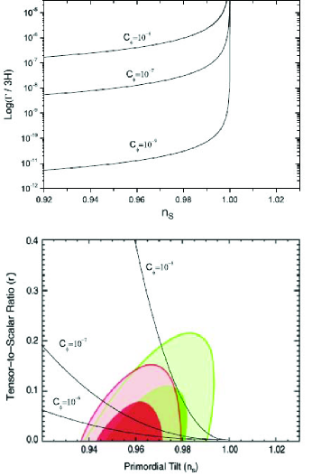
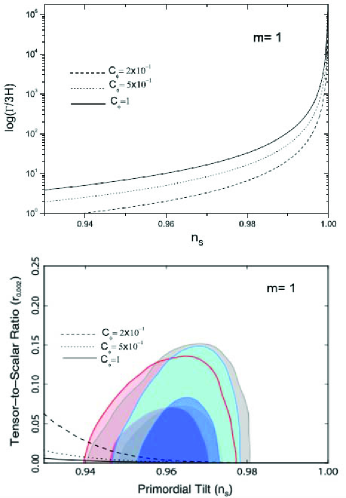
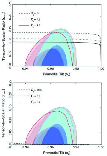
In Fig.1 we show the dependence of the ratio $R=\Gamma/3H$ and the tensor-to-scalar ratio $r$ on the primordial tilt $n_{s}$ for the special case in which we fix $m=1$, i.e., $\Gamma\propto T$, in the warm weak dissipative regime. In both panels we have used three different values of the parameter $C_{\phi}$. The upper panel shows the evolution of the rate $R=\Gamma/3H$ during the inflationary scenario and we verify that the rate $R<1$. In the lower panel, we show the two-dimensional marginalized constraints (68$\%$ and 95$\%$ C.L.) on the inflationary parameters $r$ and $n_{s}$, defined as $k_{0}=0.002Mpc^{-1}$, derived with the nine-year WMAP data with extended CMB (eCMB) (green) and eCMB+BAO+$H_{0}$ (red); see Ref.astro202 . In order to write down values for the ratio $R=\Gamma/3H$, $r$, and $n_{s}$ for the case $m=1$, we utilize Eqs. (21),(22) and (23), where $C_{\gamma}=70$, $f=0.30$, and $\kappa=1$. From the upper panel we noted that the value $C_{\phi}<10^{-6}$ is well supported by the weak regime ($R=\Gamma/3H<1$). It is interesting to note that in this case we have obtained an upper bound for the parameter $C_{\phi}$. From the lower panel we note that the value of the parameter $C_{\phi}>10^{-9}$ is well supported by the confidence levels from the nine-year WMAP data.

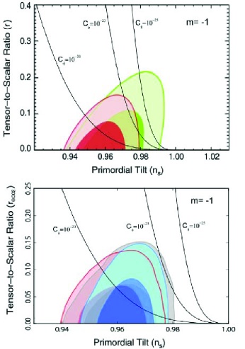
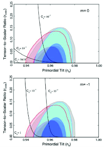
In Fig.2 we show the tensor-to-scalar ratio $r$ versus the spectral index $n_{s}$ in the warm weak dissipative regime for the case $m=-1$. In the upper panel we show the two-dimensional marginalized constraints (68$\%$ and 95$\%$ C.L.) on inflationary parameters $r$ and $n_{s}$ from nine year WMAP. In the lower panel, we shows the two-dimensional marginalized constraints (68$\%$ and 95$\%$ C.L.) from Planck in conjunction with Planck+WP Planck CMB temperature likelihood supplemented by the WMAP large-scale polarization likelihood (grey), Planck+WP+highL (red), and Planck+WP+BAO (blue) Planck . In both panels we have used three different values of the parameter $C_{\phi}$. We note that the Planck data places stronger limits on the tensor-to-scalar ratio $r$ versus $n_{s}$ compared with the nine-year WMAP data. From the lower panel in which $m=-1$, we note that for the value $C_{\phi}>10^{-25}$ the model is well supported by the Planck data. As before, we note that the value $C_{\phi}<10^{-20}$ is well supported from the condition $R<1$ ( figure not shown).

Also, in particular for the value $m=0$ in this regime, we note that for the value of the parameter $C_{\phi}>10^{-15}$ the model is well supported by the Planck data. Also, we noted that the value $C_{\phi}<10^{-11}$ is well supported from the condition $R<1$ (figure not shown). In this form, for the value $m=0$ we get $10^{-15}<C_{\phi}<10^{-11}$. We note that when we decrease the value of the parameter $m$ the values of the parameters $C_{\phi}$ also decrease.

III.2 Warm-Logamediate inflation

Assuming that the system evolves according to the weak dissipative regime and the scale factor is given by Eq.(3), then from Eqs.(8) and (3), we find the solution of the scalar field as a function of the cosmological time

$$\phi(t)=\sqrt{\frac{2\,A\,\lambda}{\kappa}}\left[\frac{2}{1+\lambda}\right](\ln t)^{\frac{1+\lambda}{2}},$$ (24)

where as before without loss of generality the integration constant $\phi_{0}=0$. The Hubble parameter $H$ as a function of the inflaton field becomes $H(\phi)=(A\,\lambda)B^{\lambda-1}\phi^{\gamma(\lambda-1)}\exp[-B\,\phi^{\gamma}],$ where the constants $\gamma$ and $B$ are given by $\gamma=\frac{2}{\lambda+1}$ and $B\equiv\left[\frac{1}{\gamma}\sqrt{\frac{\kappa}{2A\lambda}}\right]^{\gamma}$.

From Eq.(12) the effective potential with this scale factor becomes

$$V(\phi)=V_{0}\phi^{\alpha}\exp[-\beta\,\phi^{\gamma}],$$ (25)

where $V_{0}=\frac{3}{\kappa}(A\lambda)^{2}B^{2(\lambda-1)},\,\;\;\alpha=2\gamma(\lambda-1)$, and $\beta=2B$.

Note that the potential given by Eq.(25)coincides with the scalar potential obtained in Ref.R12 . Also, we note that the scalar field $\phi$, the Hubble parameter $H$, and the potential $V(\phi)$ become independent of the parameters $C_{\phi}$ and $C_{\gamma}$ in the weak regime.

Considering Eq.(11), the dissipation coefficient $\Gamma$ in terms of the scalar field is

$$\Gamma(\phi)=\,C_{\phi}^{{4\over 4-m}}\left[\frac{1}{2\kappa\,C_{\gamma}}\right]^{{m\over 4-m}}\phi^{{4(1-m)\over 4-m}}\exp[{-mB\over 4-m}\,\phi^{\gamma}].$$ (26)

For this scale factor, the dimensionless slow-roll parameter $\varepsilon$ and $\eta$ are given by $\varepsilon=-\frac{\dot{H}}{H^{2}}=(A\lambda)^{-1}B^{-(\lambda-1)}\phi^{-\gamma(\lambda-1)}$ and $\eta=-\frac{\ddot{H}}{H\dot{H}}=(A\lambda\,B^{\lambda})^{-1}\phi^{-\gamma\lambda}\left[2B\phi^{\gamma}-(\lambda-1)\right]\,.$ Analogously as before, the condition for inflation to occur is $\varepsilon<$1, and this is satisfied when $\phi>[A\lambda B^{(\lambda-1)}]^{\frac{-1}{\gamma(\lambda-1)}}$. Also considering that inflation begins at the earliest possible stage, where $\varepsilon=1$, the scalar field $\phi_{1}$ becomes $\phi_{1}=[A\lambda B^{(\lambda-1)}]^{\frac{-1}{\gamma(\lambda-1)}}\;.$

From Eq.(24), the number of $e$-folds $N$ between two different values of the scalar field $\phi_{1}$ and $\phi_{2}$ is

$$N=\int_{t_{1}}^{t_{2}}\,H\,dt=A\,\left[(\ln t_{2})^{\lambda}-(\ln t_{1})^{\lambda}\right]=AB^{\lambda}\,\left(\phi^{\gamma\lambda}_{2}-\phi^{\gamma\lambda}_{1}\right).$$ (27)

On the other hand, the density perturbation could be written from Eqs.(17) and (24) in terms of the scalar field as

$${\cal{P}_{\cal{R}}}=\frac{\kappa}{2}\left(\frac{C_{\phi}}{2\kappa C_{\gamma}}\right)^{{1\over 4-m}}(A\lambda)^{2}B^{2(\lambda-1)}\;\phi^{\alpha+{1-m\over 4-m}}\exp[-{5-m\over 4-m}B\,\phi^{\gamma}],$$ (28)

and the power spectrum in terms of the number of $e$-folds $N$ is

$${\cal{P}_{\cal{R}}}=\beta_{1}\;\left[\frac{N}{A}+(A\,\lambda)^{\frac{-\lambda}{\lambda-1}}\right]^{\frac{2(\lambda-1)}{\lambda}+{(\lambda+1)(1-m)\over 2\lambda(4-m)}}\exp\left[-{5-m\over 4-m}\left[\frac{N}{A}+(A\,\lambda)^{\frac{-\lambda}{\lambda-1}}\right]^{\frac{1}{\lambda}}\right],$$ (29)

where the constant $\beta_{1}$ is given by $\beta_{1}=\frac{\kappa}{2}\left(\frac{C_{\phi}}{2\kappa C_{\gamma}}\right)^{{1\over 4-m}}(A\lambda)^{2}B^{-{(\lambda+1)(1-m)\over 2(4-m)}}.$

The scalar spectral index $n_{s}$, from Eqs. (24) and (29), is given by

$$n_{s}=1-\frac{(5-m)B^{-(\lambda-1)}}{A\,\lambda(4-m)}\phi^{-\gamma(\lambda-1)}+\left[\frac{2(\lambda-1)}{A\lambda}+{(\lambda+1)(1-m)\over 2A\lambda(4-m)}\right]B^{-\lambda}\phi^{-\gamma\lambda}.$$ (30)

As before, we note that the scalar index can be re-expressed in terms of the number $N$ as

$$n_{s}=1-\frac{(5-m)}{A\,\lambda(4-m)}\left[\frac{N}{A}+(A\,\lambda)^{\frac{-\lambda}{\lambda-1}}\right]^{-\frac{\lambda-1}{\lambda}}+\left[\frac{2(\lambda-1)}{A\lambda}+{(\lambda+1)(1-m)\over 2A\lambda(4-m)}\right]\left[\frac{N}{A}+(A\,\lambda)^{\frac{-\lambda}{\lambda-1}}\right]^{-1},$$ (31)

where we have used Eq.(27).

For the the tensor-to-scalar ratio $r$, from Eq.(29) we have

$$r\simeq\frac{4}{\pi^{2}}\left(\frac{2\kappa C_{\gamma}}{C_{\phi}}\right)^{{1\over 4-m}}\;\phi^{-{1-m\over 4-m}}\exp\left[\left({5-m\over 4-m}-2\right)B\,\phi^{\gamma}\right].$$ (32)

Also, the tensor-to-scalar ratio as function of the number of $e$-foldings $N$ becomes

$$r\simeq\beta_{2}\;\left[\frac{N}{A}+(A\,\lambda)^{\frac{-\lambda}{\lambda-1}}\right]^{-{(\lambda+1)(1-m)\over 2\lambda(4-m)}}\exp\left[\left({5-m\over 4-m}-2\right)\left[\frac{N}{A}+(A\,\lambda)^{\frac{-\lambda}{\lambda-1}}\right]^{\frac{1}{\lambda}}\right].$$ (33)

where the constant $\beta_{2}=\frac{4}{\pi^{2}}\left(\frac{2\kappa C_{\gamma}}{C_{\phi}}\right)^{{1\over 4-m}}B^{{(\lambda+1)(1-m)\over 2(4-m)}}$.

Figure 3: The evolution of the ratio $R=\Gamma/3H$ versus the primordial tilt $n_{s}$ (upper panel) and the evolution of the tensor-to-scalar ratio r versus $n_{s}$ (lower panel) in the warm logamediate weak dissipative regime for the case $m=1$, i.e., $\Gamma\propto T$. In both panels we use three different values of the parameter $C_{\phi}$, $\kappa=1$, and $C_{\gamma}=70$. In the lower panel we show the two-dimensional marginalized constraints (68$\%$ and 95$\%$ C.L.) on the inflationary parameters $r$ and $n_{s}$, derived from Planck Planck

.

Figure 4: The upper and lower panels show the evolution of the of the tensor-to-scalar ratio r versus $n_{s}$, in the warm logamediate weak dissipative regime for the cases $m=0$ and $m=-1$, respectively. In both panels we use three different values of the parameter $C_{\phi}$, $\kappa=1$ and $C_{\gamma}=70$. In both panels we show the two-dimensional marginalized constraints (68$\%$ and 95$\%$ C.L.) on the inflationary parameters $r$ and $n_{s}$ derived from Planck Planck

.

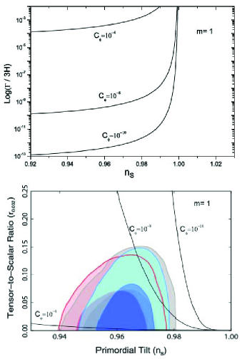
In Fig.3 we show the dependence of the ratio $R=\Gamma/3H$ and the tensor-to-scalar ratio $r$ on the primordial tilt $n_{s}$ for the special case in which we fixe $m=1$ in the warm logamediate weak dissipative regime. In both panels we use three different values of the parameter $C_{\phi}$. In the upper panel we show the decay of the ratio $R=\Gamma/3H$ during the inflationary scenario and we also verify that the rate $R<1$. In the lower panel we show the two-dimensional marginalized constraints (68$\%$ and 95$\%$ C.L.) on the inflationary parameters $r$ and $n_{s}$ derived from Planck. In order to write down values for the ratio $R=\Gamma/3H$, $r$, and $n_{s}$ for the case $m=1$, we numerically utilize Eqs. (30) and (32), where $C_{\gamma}=70$ and $\kappa=1$. Also, we numerically resolve Eqs.(29) and (31) and we find that $A=6.65\times 10^{-5}$ and $\lambda=5.03$ for the value of $C_{\phi}=10^{-4}$, in which $n_{s}=0.96$, $N=60$, and ${\cal{P}_{\cal{R}}}=2.43\times 10^{-9}$ . Analogously, for $C_{\phi}=10^{-8}$, $A=8.43\times 10^{-4}$ and $\lambda=4.36$, and for $C_{\phi}=10^{-10}$, $A=2.88\times 10^{-3}$ and $\lambda=4.02$. From the upper panel we note that the value $C_{\phi}<10^{-4}$ is well supported by the weak regime ($R=\Gamma/3H<1$). It is interesting to note that in this case we have obtained an upper bound for the parameter $C_{\phi}$. From the lower panel we note that the value of the parameter $C_{\phi}>10^{-10}$ is well supported by the confidence levels from the Planck data.

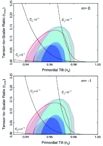
In Fig.4 we show the dependence of the tensor-to-scalar ratio on the spectral index for the weak regime in warm logamediate inflation, where as before we use three different values of the parameter $C_{\phi}$. In the upper panel we use $m=0$ and in the lower panel $m=-1$.

Regime	Scale factor	$\Gamma=C_{\phi}\frac{T^{m}}{\phi^{m-1}}$	Constraint on $C_{\phi}$
Weak	Intermediate $a(t)=e^{At^{f}}$	$m=1$ $m=0$ $m=-1$	$10^{-9}<C_{\phi}<10^{-6}$ $10^{-15}<C_{\phi}<10^{-11}$ $10^{-25}<C_{\phi}<10^{-20}$
$\Gamma<3H$	Logamediate $a(t)=e^{A(\ln t)^{\lambda}}$	$m=1$ $m=0$ $\ m=-1$	$10^{-10}<C_{\phi}<10^{-4}$ $10^{-17}<C_{\phi}<10^{-6}$ $\ 10^{-24}<C_{\phi}<10^{-10}$

Table 1: Results for the constraints on the parameter $C_{\phi}$ in the weak regime.

The Planck data places stronger limits on the tensor-to-scalar ratio $r$. In order to write down values that relate $n_{s}$ and $r$, we numerically solve Eqs.(30) and (32). Also, in both panels we have used the values $C_{\gamma}=70$ and $\kappa=1$. Here, for the rate $R=\Gamma/3H$, $r$, and $n_{s}$ for the case $m=0$, we numerically utilize Eqs. (30) and (32), where $C_{\gamma}=70$ and $\kappa=1$. Also, we numerically resolve Eqs.(29) and (31), and we find that $A=1.79\times 10^{-4}$ and $\lambda=3.78$ for the value of $C_{\phi}=10^{-9}$, where $n_{s}=0.96$, $N=60$, and ${\cal{P}_{\cal{R}}}=2.43\times 10^{-9}$. Analogously, $C_{\phi}=10^{-13}$ corresponds to $A=1.16\times 10^{-3}$ and $\lambda=4.15$, and $C_{\phi}=10^{-16}$ corresponds to $A=4.53\times 10^{-3}$ and $\lambda=4.27$. From the upper panel in which $m=0$, we note that for the value of the parameter $C_{\phi}>10^{-17}$ the model is well supported by the data in the warm logamediate weak regime. Also, we note that for $m=0$ the value $C_{\phi}<10^{-6}$ is well supported by the condition $R=\Gamma/3H<1$ (not shown). In this form, for $m=0$ the constraint for $C_{\phi}$ is given by $10^{-17}<C_{\phi}<10^{-6}$ for the weak regime in logamediate inflation. As before, for the case $m=-1$ we find that $A=3.15\times 10^{-4}$ and $\lambda=4.42$ for $C_{\phi}=10^{-14}$, where $n_{s}=0.96$, $N=60$ and ${\cal{P}_{\cal{R}}}=2.43\times 10^{-9}$. Analogously, $C_{\phi}=10^{-19}$ corresponds to $A=1.99\times 10^{-3}$ and $\lambda=3.93$ and $C_{\phi}=10^{-23}$ corresponds to $A=8.33\times 10^{-3}$ and $\lambda=3.55$. Also, from the lower panel in which $m=-1$ we note that for $C_{\phi}>10^{-24}$ the model is well supported by Planck. As before, we note that for $m=-1$ the value $C_{\phi}<10^{-10}$ is well supported by the condition $R=\Gamma/3H<1$ (not shown) and the constraint for $C_{\phi}$ is $10^{-24}<C_{\phi}<10^{-10}$. We observe that when we decrease the values of the parameter $m$ the value of $C_{\phi}$ decreases as well.

Table I indicates the constraints of the parameter $C_{\phi}$ in the weak regime and different choices of the parameter $m$, for a general form for the dissipative coefficient $\Gamma(T,\phi)=C_{\phi}\,T^{m}/\phi^{m-1}$, in the context of warm intermediate and logamediate inflationary universe models.

IV The Strong dissipative regime $\Gamma>3H$

IV.1 Warm-Intermediate inflation

We now analyze the case of the strong dissipative regime ($R=\Gamma/3H>1$), together with the scale factor given by Eq.(2), i.e., intermediate inflation. From Eqs.(8) and (11) we get $\dot{\phi}\phi^{\frac{1-m}{2}}=k_{6}t^{\beta_{6}},$ where $k_{6}=\left[\frac{2}{\kappa\alpha_{m}}(\left[3(1-f)\right]^{4-m}(Af)^{8-m})^{\frac{1}{4}}\right]^{\frac{1}{2}}$ and $\beta_{6}=\frac{1}{8}\left[f(8-m)+2m-12\right]$. In this way, the solution of the scalar field $\phi(t)$ is given by

$$\phi(t)-\phi_{0}=k_{7}\,t^{\frac{f(8-m)+2m-4}{4(3-m)}},$$ (34)

where the constant $k_{7}=\left[\frac{4k_{6}(3-m)}{f(8-m)+2m-4}\right]^{\frac{2}{3-m}}$ and $\phi(t=0)=\phi_{0}$ is an integration constant. As before, without loss of generality, we consider $\phi_{0}=0$. The Hubble parameter as a function of the inflaton field is given by $H(\phi)=Af\left(\frac{\phi}{k_{7}}\right)^{\frac{-4(1-f)(3-m)}{f(8-m)+2m-4}}.$

From Eq.(12) the scalar potential as a function of the scalar field is

$$V(\phi)=\frac{3\left(Af\right)^{2}}{\kappa}k_{7}^{\frac{8(1-f)(3-m)}{f(8-m)+2m-4}}\phi^{\frac{-8(1-f)(3-m)}{f(8-m)+2m-4}}.$$ (35)

Here we note that in the case of the strong regime the scalar field $\phi$, the Hubble parameter $H$, and the potential $V(\phi)$ now depend on the parameters $C_{\phi}$ and $C_{\gamma}$.

The dissipation coefficient $\Gamma$ in terms of the scalar field considering Eq.(11) is given by

$$\Gamma(\phi)=k_{8}\phi^{\beta_{7}},$$ (36)

where the constants $k_{8}$ and $\beta_{7}$ are defined as $k_{8}=\alpha_{m}3^{\frac{m}{4}}\left[Af(1-f)\right]^{\frac{m}{4}}k_{7}^{\frac{m(2-f)(3-m)}{f(8-m)+2m-4}}$ and $\beta_{7}=\frac{f(8-6m)-4}{f(8-m)+2m-4}$.

For this regime, the dimensionless slow-roll parameter $\varepsilon$ becomes $\varepsilon=-\frac{\dot{H}}{H^{2}}=\frac{(1-f)}{Af}\left(\frac{\phi}{k_{7}}\right)^{-\beta_{8}},$ where the constant $\beta_{8}=\frac{4f(3-m)}{f(8-m)+2m-4}$. As before, the condition for inflation to occur is only satisfied when $\phi>k_{7}\left(\frac{1-f}{Af}\right)^{\frac{1}{\beta_{8}}}.$ Also, considering that inflation begins at the earliest possible stage (where $\varepsilon=1$), we get $\phi_{1}=k_{7}\left(\frac{1-f}{Af}\right)^{\frac{1}{\beta_{8}}}.$

In this regime, the number of $e$-folds $N$ between two different values of the scalar field $\phi_{1}$ and $\phi_{2}$ from Eq.(34) is

$$N=\int_{t_{1}}^{t_{2}}\,H\,dt=A\,\left(t_{2}^{f}-t_{1}^{f}\right)=Ak_{7}^{-\beta_{8}}\left[\phi_{2}^{\beta_{8}}-\phi_{1}^{\beta_{8}}\right].$$ (37)

On the other hand, as the scalar perturbations, ${\mathcal{P}_{\mathcal{R}}}^{1/2}\propto\frac{H}{\dot{\phi}}\,\delta\phi$, where now $\delta\phi^{2}$ in the strong dissipation regime is given by, $\delta\phi^{2}\simeq\frac{k_{F}T}{2\pi^{2}}$; see Ref.taylorberera . Here $k_{F}$ is the wave-number and it is given by $k_{F}=\sqrt{\Gamma H}=H\sqrt{3R}$. In this form, by combining the Eqs.(8), (10), and (11), the expression for the spectrum of the scalar perturbation can be written as

$$P_{\mathcal{R}}\simeq\frac{H^{\frac{5}{2}}\Gamma^{\frac{1}{2}}T}{2\pi^{2}\dot{\phi}^{2}}=\frac{\kappa C_{\phi}^{\frac{3}{2}}3^{\frac{3m-6}{8}}}{4\pi^{2}\left(2\kappa C_{\gamma}\right)^{\frac{3m+2}{8}}}H^{\frac{3}{2}}\left(-\dot{H}\right)^{\frac{3m-6}{8}}\phi^{\frac{3(1-m)}{2}}.$$ (38)

By using Eqs. (34) and (38), the power spectrum in terms of the scalar field can be written as

$$P_{\mathcal{R}}=k_{9}\phi^{-\beta_{9}},$$ (39)

where $k_{9}=\frac{\kappa C_{\phi}^{\frac{3}{2}}3^{\frac{3m-6}{8}}\left(Af\right)^{\frac{3m+6}{8}}\left(1-f\right)^{\frac{3m-6}{8}}}{4\pi^{2}\left(2\kappa C_{\gamma}\right)^{\frac{3m+2}{8}}}k_{7}^{\frac{3}{2}(1-m)+\beta_{9}}$ and $\beta_{9}=\frac{3(2+f(4m-7))}{f(8-m)+2m-4}.$

The scalar spectral index $n_{s}=n_{s}(\phi)$ from Eqs. (34) and (39) is

$$n_{s}=1-\frac{3\left[2+f(4m-7)\right]}{4Af(3-m)}k_{7}^{\beta_{8}}\phi^{-\beta_{8}}.$$ (40)

Note that the spectral index, can also be re-expressed in terms of the number of $e$-foldings. Combining Eqs.(37) and (40), the spectral index becomes

$$n_{s}=1-\frac{3(2+f(4m-7))}{4(3-m)(1+f(N-1))}.$$ (41)

As before, here the value of $f$ in terms of $m$, $n_{s}$, and $N$ from Eq.(41) is given by $f=\frac{4(1-n_{s})(3-m)-6}{3(4m-7)-4(3-m)(1-n_{s})(N-1)}.$ In particular, for the values $m=1$, $n_{s}=0.96$, and $N=60$ we obtain $f\simeq 0.21$. Analogously, $m=0$ corresponds to $f\simeq 0.11$, and $m=-1$ corresponds to $f\simeq 0.08$.

Analogously to the case of the intermediate weak regime, we can obtain an analytic expression for the parameter $A$ in terms of the parameters $C_{\phi}$, $C_{\gamma}$, ${\mathcal{P}_{\mathcal{R}}}$, $m$, $n_{s}$, and $N$. Considering Eqs.(37) and (39), we get

$$A=\frac{1}{f}\left(\frac{{\mathcal{P}_{\mathcal{R}}}}{k_{10}}\right)^{\frac{2f(3-m)}{3}}\left[f(N-1)+1\right]^{\frac{2+f(4m-7)}{2}},$$ (42)

where the constant $k_{10}=\frac{\kappa C_{\phi}^{\frac{3}{2}}3^{\frac{3m-6}{8}}\left(Af\right)^{\frac{3m+6}{8}}\left(1-f\right)^{\frac{3m-6}{8}}}{4\pi^{2}\left(2\kappa C_{\gamma}\right)^{\frac{3m+2}{8}}}\left[\frac{\beta_{8}}{f}\left(\frac{2}{\kappa\alpha_{m}}\left[3(1-f)\right]^{\frac{4-m}{4}}\right)^{\frac{1}{2}}\right]^{\frac{3(1-m)}{3-m}}.$ In particular, $m=1$, where $f\simeq 0.21$, $n_{s}=0.96$, $C_{\gamma}=70$, ${\mathcal{P}_{\mathcal{R}}}=2.4\times 10^{-9}$, and $N=60$, we obtain that $A\simeq 1.76$ when $C_{\phi}=2\times 10^{-1}$, $A=1.21$ when $C_{\phi}=5\times 10^{-1}$, and $A=0.92$ when $C_{\phi}=1$ . Analogously, for $m=0$, $A=10.33$ when $C_{\phi}=10^{-5}$, $A=3.68$ when $C_{\phi}=10^{-3}$, and $A=1.54$ when $C_{\phi}=5\times 10^{-2}$. Finally, for $m=-1$, $A=22.40$ when $C_{\phi}=10^{-9}$, $A=5.55$ when $C_{\phi}=10^{-5}$, $A=0.97$ when $C_{\phi}=1$.

Also, we can find an expression for the rate $R=\Gamma/3H$ in terms of the scalar spectral index. By using Eqs.(36) and (40) the ratio $R$ has the following dependence on $n_{s}$:

$$R(n_{s})=\frac{k_{8}k_{7}^{\beta_{7}}}{3Af}\left(\frac{3\left[2+f(4m-7)\right]}{4Af(3-m)(1-n_{s})}\right)^{-\frac{\left[4(m-2)+2f(m+2)\right]}{4f(3-m)}}.$$ (43)

Figure 5: The evolution of the ratio $\log(\Gamma/3H)$ versus the primordial tilt $n_{s}$ (upper panel) and the evolution of the tensor-to-scalar ratio r versus $n_{s}$ (lower panel) in the warm intermediate strong dissipative regime for the case $m=1$, i.e., $\Gamma\propto T$. In both panels we use three different values of the parameter $C_{\phi}$, and $\kappa=1$ and $C_{\gamma}=70$. In the lower panel we show the two-dimensional marginalized constraints (68$\%$ and 95$\%$ C.L.) on the inflationary parameters $r$ and $n_{s}$ derived from Planck Planck

.

Figure 6: The upper and lower panel show the evolution of the tensor-to-scalar ratio r versus $n_{s}$ in the warm intermediate strong dissipative regime for the cases $m=0$ and $m=-1$, respectively. As before, In both panels, we use three different values of the parameter $C_{\phi}$, and $\kappa=1$ and $C_{\gamma}=70$. Also, in both panels we show the two-dimensional marginalized constraints (68$\%$ and 95$\%$ C.L.) on the inflationary parameters $r$ and $n_{s}$ derived from Planck; see Ref.Planck

.

On the other hand, for the intermediate strong dissipative regime, the tensor-to-scalar ratio $r=r(\phi)$ from Eqs.(34) and (39) is

$$r(\phi)=\left(\frac{{\mathcal{P}}_{g}}{P_{\mathcal{R}}}\right)\simeq\frac{2\kappa\left(Af\right)^{2}k_{7}^{\beta_{10}}}{\pi^{2}k_{9}}\phi^{\beta_{11}},$$ (44)

where the constants $\beta_{10}$ and $\beta_{11}$ are defined as $\beta_{10}=\frac{8(1-f)(3-m)}{f(8-m)+2m-4}$ and $\beta_{11}=\frac{3(f-6)+4m(2+f)}{f(8-m)+2m-4}$.

Also, the tensor-to-scalar ratio can be written in terms of the scalar spectral index $n_{s}$ as

$$r(n_{s})=\frac{2\kappa\left(Af\right)^{2}k_{7}^{\beta_{10}+\beta_{11}}}{\pi^{2}k_{9}}\left[\frac{3\left[2+f(4m-7)\right]}{4Af(3-m)(1-n_{s})}\right]^{\frac{3(f-6)+4m(2+f)}{4f(3-m)}},$$ (45)

and also the tensor-to-scalar ratio as a function of the number of $e$-foldings $N$ is

$$r(N)=\frac{2\kappa(Af)^{2}k_{7}^{\beta_{10}+\beta_{11}}}{\pi^{2}k_{9}}\left[\frac{f(N-1)+1}{Af}\right]^{\frac{3(f-6)+4m(2+f)}{4f(3-m)}}.$$ (46)

In Fig.5, we show the dependence of the ratio $\log(\Gamma/3H)$ and the tensor-scalar ratio $r$ on the primordial tilt $n_{s}$ for the special case in which we fix $m=1$ in the warm intermediate strong dissipative regime. As before, in both panels we have used three different values of the parameter $C_{\phi}$. In the upper panel we show the decay of the ratio $R=\Gamma/3H$ during the inflationary scenario and we verify that the rate $R<1$. In the lower panel we show the two-dimensional marginalized constraints (68$\%$ and 95$\%$ C.L.) on the inflationary parameters $r$ and $n_{s}$ derived from PlanckPlanck . In order to write down values for the ratio $R=\Gamma/3H$, $r$, and $n_{s}$ for the case $m=1$, we consider Eqs. (43) and (45) (where $C_{\gamma}=70$,$\kappa=1$) and the values of $f$ and $A$ for $m=1$ obtained from Eqs.(41) and (42). From the upper panel we note that the value $C_{\phi}>2\times 10^{-1}$ is well supported by the strong regime ($R=\Gamma/3H>1$). From the lower panel we note that the value $C_{\phi}<1$ is well supported by the confidence levels from Planck. In this form, the range of the parameter $C_{\phi}$ for the value $m=1$ is $2\times 10^{-1}<C_{\phi}<1$.

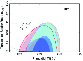
In Fig.6, we show the dependence of the tensor-to-scalar ratio $r$ on the primordial tilt $n_{s}$ for the cases $m=0$ and $m=-1$ in the warm intermediate strong dissipative regime. As before, in both panels we have used three different values of the parameter $C_{\phi}$. In both panels, we show the two-dimensional marginalized constraints (68$\%$ and 95$\%$ C.L.) on the inflationary parameters $r$ and $n_{s}$ derived from Planck. In order to write down values for $r$ and $n_{s}$ for each value of $m$, we use Eq. (45) (where $C_{\gamma}=70$,$\kappa=1$) and the values of $f$ and $A$ for each value of $m$ and $C_{\phi}$ obtained from Eqs.(41) and (42). From the upper panel in which $m=0$, we note that the value $C_{\phi}<10^{-2}$ is well supported by the confidence levels from the Planck data. Also, we observe that the value $C_{\phi}>10^{-6}$ is well supported by the strong regime, i.e., $R=\Gamma/3H>1$ (not shown). In this form, the range of the parameter $C_{\phi}$ for $m=0$, is $10^{-6}<C_{\phi}<10^{-2}$. From the lower panel we note that the value $C_{\phi}<1$ is well supported by the confidence levels from the Planck data. Also, we note that the value $C_{\phi}>10^{-11}$ is well supported by the strong regime, i.e., $R=\Gamma/3H>1$ (also not shown). In this way, the range of the parameter $C_{\phi}$ for $m=-1$ is $10^{-11}<C_{\phi}<1$.

IV.2 Warm logamediate inflation

We now consider the case of the strong regime together with $a(t)$ given by Eq.(3). From Eq.(8), the solution of $\phi(t)$ is given by

$$\varphi(t)\equiv\left({2\over 3-m}\right)\phi(t)^{{3-m\over 2}}\,=\alpha_{1}\ \gamma_{m}[t],$$ (47)

where the constant $\alpha_{1}$ is defined by $\alpha_{1}={(4C_{\gamma})^{m/8}\over C_{\phi}^{1/2}}\left({6\over\kappa}\right)^{{4-m\over 8}}(A\,\lambda)^{{8-m\over 8}}\left({4\over 2-m}\right)^{1+\frac{8-m}{8}(\lambda-1)},$ and the function

$$\gamma_{m}[t]\equiv\,\gamma\left[1+\frac{8-m}{8}(\lambda-1),\frac{2-m}{4}\ln t\right]$$

is the incomplete gamma function; see,e.g., Refs.Libro ; Libro02 . The Hubble parameter $H=H(\phi)$ is given by the expression $H(\phi)=A\,\lambda\,\left(\gamma_{m}^{-1}\left[\varphi/\alpha_{1}\right]\right)^{-1}\left(\ln\gamma_{m}^{-1}\left[\varphi/\alpha_{1}\right]\right)^{\lambda-1},$ where $\gamma_{m}^{-1}\left[\varphi/\alpha_{1}\right]$ denotes the inverse gamma function of $\gamma_{m}[t]$.

Analogous to the case of the logamediate weak dissipative regime, the scalar potential from Eq.(12) becomes

$$V(\varphi)=\frac{3}{\kappa}(A\,\lambda)^{2}\left(\gamma_{m}^{-1}\left[\varphi/\alpha_{1}\right]\right)^{-2}\left(\ln\gamma_{m}^{-1}\left[\varphi/\alpha_{1}\right]\right)^{2(\lambda-1)},$$ (48)

and the dissipation coefficient $\Gamma=\Gamma(\phi)$ from Eq.(11) is

$$\Gamma(\phi)=C_{\phi}\left[\frac{3}{2\kappa\,C_{\gamma}}\right]^{m/4}(A\lambda)^{m/4}\phi^{1-m}\left(\gamma_{m}^{-1}\left[\varphi/\alpha_{1}\right]\right)^{-m/2}\left(\ln\gamma_{m}^{-1}\left[\varphi/\alpha_{1}\right]\right)^{\frac{m}{4}(\lambda-1)}.$$ (49)

As before, the dimensionless slow-roll parameter $\varepsilon$ for this regime becomes $\varepsilon=-\frac{\dot{H}}{H^{2}}=(A\lambda)^{-1}\left(\ln\gamma_{m}^{-1}\left[\varphi/\alpha_{1}\right]\right)^{-(\lambda-1)},$ and the slow-roll parameter $\eta=-\frac{\ddot{H}}{H\dot{H}}=(A\lambda)^{-1}\left(\ln\gamma_{m}^{-1}\left[\varphi/\alpha_{1}\right]\right)^{-\lambda}\left\{2\left(\ln\gamma_{m}^{-1}\left[\varphi/\alpha_{1}\right]\right)-(\lambda-1)\right\}.$

Again, following Ref.R12 , the condition $\varepsilon=1$ at the beginning of inflation the scalar field gives

$$\varphi_{1}=\left({2\over 3-m}\right)\,\phi_{1}^{{3-m\over 2}}=\alpha_{1}\;\gamma_{m}\left[\exp[(A\lambda)^{\frac{-1}{\lambda-1}}]\right],$$ (50)

The number of $e$-folds $N$ in this regime from Eq.(47) is given by

$$N=\int_{t_{1}}^{t_{2}}\,H\,dt=A\,\left\{\left(\ln\gamma_{m}^{-1}\left[\varphi_{2}/\alpha_{1}\right]\right)^{\lambda}-\left(\ln\gamma_{m}^{-1}\left[\varphi_{1}/\alpha_{1}\right]\right)^{\lambda}\right\}.$$ (51)

From Eqs.(38) and (47) we obtain that ${\cal{P}_{\cal{R}}}$ in terms of the scalar field becomes

$${\cal{P}_{\cal{R}}}=\alpha_{2}\,\phi^{{3(1-m)\over 2}}\,\left(\gamma_{m}^{-1}\left[\varphi/\alpha_{1}\right]\right)^{-{3m\over 4}}\left(\ln\gamma_{m}^{-1}\left[\varphi/\alpha_{1}\right]\right)^{\frac{3m+6}{8}(\lambda-1)},$$ (52)

where the constant $\alpha_{2}$ is given by $\alpha_{2}=\frac{\kappa}{4\pi^{2}}3^{{3m-6\over 8}}C_{\phi}^{3/2}\left(\frac{1}{2\kappa C_{\gamma}}\right)^{{3m+2\over 8}}(A\lambda)^{{3m+6\over 8}}.$

Also, as before the scalar spectrum can be re-expressed in terms of the number of e-folding $N$, as

$${\cal{P}_{\cal{R}}}(N)=\alpha_{2}\,\left[\frac{N}{A}+(A\,\lambda)^{\frac{-\lambda}{\lambda-1}}\right]^{{(3m+6)(\lambda-1)\over 8\lambda}}\exp\left[-{3m\over 4}\left[\frac{N}{A}+(A\,\lambda)^{\frac{-\lambda}{\lambda-1}}\right]^{\frac{1}{\lambda}}\right]\,F_{m}(N),$$ (53)

where the function $F_{m}(N)=\left[\alpha_{1}\,\left({3-m\over 2}\right)\,\gamma_{m}(\exp\left[\left[\frac{N}{A}+(A\,\lambda)^{\frac{-\lambda}{\lambda-1}}\right]^{\frac{1}{\lambda}}\right])\right]^{{3(1-m)\over 3-m}}.$

Considering Eqs.(47) and (49), the scalar spectral index $n_{s}$ is given by

$$n_{s}=1-\frac{3m}{4A\lambda}\left(\ln\gamma_{m}^{-1}\left[\varphi/\alpha_{1}\right]\right)^{-(\lambda-1)}+\frac{(3m+6)(\lambda-1)}{8A\lambda}\left(\ln\gamma_{m}^{-1}\left[\varphi/\alpha_{1}\right]\right)^{-\lambda}+K\,G_{m}(\phi).$$ (54)

where the constant $K$ is defined as $K={3(1-m)\over 2}C_{\phi}^{-1/2}\left(4C_{\gamma}\right)^{{m\over 8}}\left(\frac{6}{\kappa}\right)^{{4-m\over 8}}(A\lambda)^{-{m\over 8}}$ and the function $G_{m}(\phi)=\phi^{{m-3\over 2}}\,\left(\gamma_{m}^{-1}\left[\varphi/\alpha_{1}\right]\right)^{{m-2\over 4}}\left(\ln\gamma_{m}^{-1}\left[\varphi/\alpha_{1}\right]\right)^{-\frac{m}{8}(\lambda-1)}$.

Analogously, as before the scalar spectral index can be write in terms of the number of $e$-folds. Considering Eqs. (50) and (51), we obtain

$$n_{s}=1-\frac{3m}{4A\,\lambda}\left[\frac{N}{A}+(A\,\lambda)^{\frac{-\lambda}{\lambda-1}}\right]^{-\frac{\lambda-1}{\lambda}}+\frac{(3m+6)(\lambda-1)}{8A\,\lambda}\left[\frac{N}{A}+(A\,\lambda)^{\frac{-\lambda}{\lambda-1}}\right]^{-1}+K\,J_{m}(N),$$ (55)

where $J_{m}(N)=\left[\frac{N}{A}+(A\,\lambda)^{\frac{-\lambda}{\lambda-1}}\right]^{{-m(\lambda-1)\over 8\lambda}}\exp\left[{m-2\over 4}\left[\frac{N}{A}+(A\,\lambda)^{\frac{-\lambda}{\lambda-1}}\right]^{\frac{1}{\lambda}}\right]\,j_{m}(N)$ and the function $j_{m}(N)$ is given by $j_{m}(N)=\left[\alpha_{1}{3-m\over 2}\gamma_{m}[\exp\left[\left[\frac{N}{A}+(A\,\lambda)^{\frac{-\lambda}{\lambda-1}}\right]^{\frac{1}{\lambda}}\right]]\right]^{-1}.$

For this regime and scale factor, we may write the tensor-to-scalar ratio as

$$r=\,\alpha_{3}\,\phi^{{3(m-1)\over 2}}\,\left(\gamma_{m}^{-1}\left[\varphi/\alpha_{1}\right]\right)^{{3m-8\over 4}}\left(\ln\gamma_{m}^{-1}\left[\varphi/\alpha_{1}\right]\right)^{\frac{10-3m}{8}(\lambda-1)},$$ (56)

where the constant $\alpha_{3}=\frac{2\kappa(A\lambda)^{2}}{\pi^{2}\alpha_{2}}$. Also, we can write the tensor-to-scalar ratio as a function of the number of $e$-foldings $N$ as

$$r=\alpha_{3}\,\left[\frac{N}{A}+(A\,\lambda)^{\frac{-\lambda}{\lambda-1}}\right]^{{(10-3m)(\lambda-1)\over 8\lambda}}\exp\left[{3m-8\over 4}\left[\frac{N}{A}+(A\,\lambda)^{\frac{-\lambda}{\lambda-1}}\right]^{\frac{1}{\lambda}}\right]\,{1\over F_{m}(N)}.$$ (57)

In Fig.7, we show the dependence of the tensor-to-scalar ratio $r$ on the primordial tilt $n_{s}$ for the special case in which we fix $m=1$ in the warm logamediate strong dissipative regime. Here, we use two different values of the parameter $C_{\phi}$, and we also show the two-dimensional marginalized constraints (68$\%$ and 95$\%$ C.L.) on the inflationary parameters $r$ and $n_{s}$ derived from PlanckPlanck . In order to write down values for the ratio $r$ and $n_{s}$ for the case $m=1$, we numerically utilize Eqs. (54) and (56), where $C_{\gamma}=70$ and $\kappa=1$. Also, we numerically resolve Eqs.(29) and (31) and we find that $A=2.01\times 10^{-3}$ and $\lambda=3.71$ for the value of $C_{\phi}=10^{-1}$, for which $n_{s}=0.96$, $N=60$, and ${\cal{P}_{\cal{R}}}=2.43\times 10^{-9}$. Analogously, $C_{\phi}=7\times 10^{-2}$ corresponds to $A=3.53\times 10^{-3}$ and $\lambda=3.56$. From the plot we note that the value $C_{\phi}<10^{-1}$ is well supported by the confidence levels from the Planck data, since for values of $C_{\phi}>10^{-1}$ the ratio $r\sim 0$. Also, we note that the value of the parameter $C_{\phi}>7\times 10^{-2}$ is well supported by the strong regime, i.e., $R=\Gamma/3H>1$ (not shown). In this way, the range for the parameter $C_{\phi}$ in the special case in which $m=1$ is $7\times 10^{-2}<C_{\phi}<10^{-1}$.

Figure 7: The plot shows the evolution of the of the tensor-to-scalar ratio r versus $n_{s}$ in the warm logamediate strong dissipative regime for the case $m=1$. Here we use two different values of the parameter $C_{\phi}$, and $\kappa=1$ and $C_{\gamma}=70$. We show the two-dimensional marginalized constraints (68$\%$ and 95$\%$ C.L.) on the inflationary parameters $r$ and $n_{s}$ derived from Planck dataPlanck .

Also, we note that for the cases in which $m=0$ and $m=-1$ the models of the warm logamediate strong regime are disfavored from the observational data, since the spectral index $n_{s}>1$, see Eq.(55)) and the models do not work.

Regime	Scale factor	$\Gamma=C_{\phi}\frac{T^{m}}{\phi^{m-1}}$	Constraint on $C_{\phi}$
Strong	Intermediate $a(t)=e^{At^{f}}$	$m=1$ $m=0$ $\ m=-1$	$2\times 10^{-1}<C_{\phi}<1$ $\ \ \ \ \ \ \ \ \ \ \ \ 10^{-6}<C_{\phi}<10^{-2}$   $\ \ \ \ 10^{-11}<C_{\phi}<1$
$\Gamma>3H$	Logamediate $a(t)=e^{A(\ln t)^{\lambda}}$	$\ m=1$ $m=0$ $\ m=-1$	$\ \ \ \ \ \ 7\times 10^{-2}<C_{\phi}<10^{-1}$               The model does not work             The model does not work

Table 2: Results for the constraints on the parameter $C_{\phi}$ in the strong regime.

Table II indicates the constraints on the parameter $C_{\phi}$ in the strong regime and different choices of the parameter $m$, for a general form for the dissipative coefficient $\Gamma(T,\phi)=C_{\phi}\,T^{m}/\phi^{m-1}$, in the context of warm intermediate and logamediate inflationary universe models.

V Interpolation between the weak and strong decays

Given that the ratio $R=\Gamma/3H$ will also evolve during inflation, we may also hace models where we start with the weak regime ($R<1$) but end in the strong regime ($R>1$).

In the following, we will analyze the intermediate and logamediate models in the context of the interpolation between the weak and strong decays only for the value $m=1$. For the values $m=0$ and $m=-1$, we cannot find analytical solutions for the dissipation coefficient given by Eq.(11). For this reason, we will restrict ourselves to the case $m=1$.

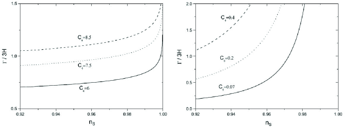
From Eq.(11) and considering the case $m=1$ together with the intermediate and logamediate models, we obtain a real solution for the dissipation coefficient $\Gamma$ as a function of time, i.e., $\Gamma=\Gamma(t)$, for each of the models. In Fig.8, we show the dependence of the ratio $R=\Gamma/3H$ and the tensor-to-scalar ratio $r$ on the primordial tilt $n_{s}$ for the special case in which we fix $m=1$ in the warm weak strong dissipative regime for the intermediate and logamediate models. In both panels we use three different values of the parameter $C_{\phi}$. The upper panel shows the evolution of the rate $R=\Gamma/3H$ during the warm intermediate model and we verify the evolution of the rate $R$ from the weak and strong decays. Here we observe that the value $C_{\phi}<10$ is well supported from the interpolation $R<1$ and $R>1$. The lower panel shows the evolution of the rate $R=\Gamma/3H$ during the warm logamediate scenario, and as before we verify the evolution of the rate $R$. Also, we note that the value $C_{\phi}<1$ is well supported from the interpolation $R<1$ and $R>1$. For values of $C_{\phi}<10^{-2}$ we find that the model evolves according to the the weak dissipative regime, i.e., $R<1$.

Figure 8: The panel on the left shows the evolution of the ratio $R=\Gamma/3H$ versus the primordial tilt $n_{s}$ in the interpolation between the weak and strong decays for the warm intermediate model, and the right panel shows the evolution of $R=\Gamma/3H$ versus $n_{s}$ for the warm logamediate model. In both panels we use three different values of the parameter $C_{\phi}$, and $m=1$, $\kappa=1$ and $C_{\gamma}=70$. Also, in the left panel we use $A=0.4$ and $f=0.9$, and in the right panel we use $A=0.002$ and $\lambda=4$.

In the following, we will describe the scalar and tensor perturbations for our warm model during the interpolation between the weak and strong decays. For a standard scalar field the density perturbation between the weak and strong regime can be written as warm

$${\cal{P}_{\cal{R}}}=\frac{\sqrt{3\,\pi}}{2}\,\frac{H^{3}\,T}{\dot{\phi}^{2}}\,(1+R)^{1/2}.$$ (58)

By using Eqs.(8) and (10) the density perturbation can be written as

$${\cal{P}_{\cal{R}}}=\sqrt{\pi}\,H^{3}\,\left[\frac{3^{3}\,\kappa^{3}}{2^{9}}\,\frac{R\,(1+R)^{5}}{C_{\gamma}\,(-\dot{H})^{3}}\right]^{1/4},$$ (59)

and the tensor-to-scalar ratio becomes

$$r\simeq\frac{1}{H}\,\left[\frac{2^{13}}{3^{3}\,\pi^{10}\,\kappa}\,\frac{C_{\gamma}\,(-\dot{H})^{3}}{R\,(1+R)^{5}}\right]^{1/4}.$$ (60)

In Fig.9 we show the dependence of the tensor-to-scalar ratio $r$ on the spectral index $n_{s}$ during the interpolation between the weak and strong dissipative regimes for the case $m=1$. In both panels we show the two-dimensional marginalized constraints (68$\%$ and 95$\%$ C.L.) on the inflationary parameters $r$ and $n_{s}$ from Planck dataPlanck for the warm intermediate and warm logamediate models. As before, in both panels we use three different values of the parameter $C_{\phi}$.

Figure 9: The upper and lower panels show the evolution of the of the tensor-to-scalar ratio r versus $n_{s}$ in the interpolation between the weak and strong decays for the warm intermediate and warm logamediate models, respectively. As before, in both we use three different values of the parameter $C_{\phi}$, and $m=1$, $\kappa=1$, and $C_{\gamma}=70$. In both panels we show the two-dimensional marginalized constraints (68$\%$ and 95$\%$ C.L.) on the inflationary parameters $r$ and $n_{s}$ derived from Planck Planck . As before, in the upper panel we use $A=0.4$ and $f=0.9$, and in the lower panel we use $A=0.002$ and $\lambda=4$.

From the upper panel, in the which the scale factor grows with the intermediate expansion, we note that for the values of $C_{\phi}>1$ the model is well supported by the Planck data. Here we observe that the curves $r=r(n_{S})$ for Planck data enter the 95$\%$ confidence region only. From the lower panel, in the which the scale factor growths with the logamediate expansion, we note that for the values of $C_{\phi}>10^{-2}$ the model is well supported by the Planck data. Also, we note that in this model the curves $r=r(n_{s})\sim 0$. In this form, for the value $m=1$, we get $1<C_{\phi}<10$ for the warm intermediate model and $10^{-2}<C_{\phi}<1$ for the warm logamediate model.

VI Conclusions

In this paper we have investigated the intermediate and logamediate inflationary model in the context of warm inflation. In the slow-roll approximation we have found solutions of the Friedmann equations for a flat universe containing a standard scalar field in the weak and strong regime for a general form of the dissipative coefficient $\Gamma(T,\phi)=C_{\phi}\,T^{m}/\phi^{m-1}$. In particular, we studied the values $m=1$, $m=0$, and $m=-1$. From the warm intermediate and logamediate inflationary models, we have obtained explicit expressions for the corresponding scalar potential, power spectrum of the curvature perturbations, tensor-to-scalar ratio and scalar spectrum index.

For both regimes, we have considered the constraints on the parameters of the models from the WMAP nine-year data and Planck data. Here we have taken the constraint $r$-$n_{s}$ plane at lowest order in the slow-roll approximation. Also, we found a constraint for the value of $C_{\phi}$ from the weak (strong) regime $R=\Gamma/3H<1$ ( $R=\Gamma/3H>1$ ). It is interesting to note that in general we have obtained an upper bound for the parameter $C_{\phi}$ from this condition. Also, we noted that when we decrease the value of the parameter $m$ the value of the parameter $C_{\phi}$ also decreases. Our results are summarized in Tables I and Table II, respectively.

During the interpolation between weak and strong decays, we analyzed the constraints on the parameters from Planck data only for the case $m=1$ in the warm intermediate and the warm logamediate models.