Simulating Bell violations without quantum computers
Abstract
We demonstrate that it is possible to simulate Bell violations using probabilistic methods. A quantum state corresponding to optical experiments that violate the Bell inequality is generated, demonstrating that these quantum paradoxes can indeed be simulated probabilistically. This provides an explicit counter-example to Feynman’s claim that such classical simulations could not be carried out.
1 Introduction
The simulation of quantum dynamics is a hard problem in physics for systems with many degrees of freedom. While large classical systems can be readily simulated with computers, this is difficult with large quantum systems due to the exponentially growing size of Hilbert space. Since an expansion in eigenstates of the Hamiltonian is virtually impossible for many-body systems, one possible solution is to use probabilistic sampling. This approach was apparently ruled out by a claim of Feynman [1], where he asked
Can quantum systems be probabilistically simulated by a classical computer?
His answer to the question was:
If you take the computer to be the classical kind and there’s no changes in any laws, and there’s no hocus-pocus, the answer is certainly, No!
This led Feynman to propose the use of quantum computers for these types of simulation, and his argument has motivated extensive research on quantum computing. However, large-scale quantum computers are not yet available. An important question therefore is whether probabilistic simulation with classical computers are truly excluded, as this claim would certainly imply. Is there some way that one can in fact use probabilistic sampling with existing digital computers for these challenging tasks? And if so, to what degree of practicality?
Given the known decoherence problems in constructing quantum computing hardware for quantum simulations, practical alternative strategies using software would be extremely useful. Here we demonstrate, by carrying out a simulation, that Bell’s theorem does not rule out probabilistic simulation methods. Our results treat the case considered by Feynman, which is a four mode photonic state used in experimental demonstrations, equivalent to two correlated spin-half particles.
This allows us to demonstrate, by means of explicit, direct computer simulation, that the answer to Feynman’s original question is actually “Yes”. Our main emphasis is the fundamental question of whether it is possible to probabilistically treat Bell violations, which was claimed to be impossible in this early literature. In fact, the “not so black and white” nature of Feynman’s claim was always apparent, given the existence of positive phase space methods that were known at the time. It was sometimes interpreted that these methods would only be useful for semiclassical states, rather than the Bell state. We show this is not so by carrying out localized probabilistic sampling of a Bell-violating quantum state for the first time, using random sampling to obtain results in complete agreement with quantum mechanics.
One may ask then, in Feynman’s words: what is the “hocus-pocus” that allows these simulations? Very simply, we only require that average correlations of the simulation outputs correspond to quantum mechanics. We do not ask the measurement values and their probabilities to be exactly identical to quantum mechanics. This allows us to average over probabilities of phase-space variables whose values are not integer eigenvalues. Another possible way to overcome this argument could be to treat nonlocal simulation, which exploits another loophole in Feynman’s logic: a simulation doesn’t have to satisfy locality. We do not investigate this option here, since our simulations use local variables, although removing this restriction may provide additional resources.
We use positive phase-space distributions of quantum mechanics for our purpose [2, 3]. These exist for every quantum state, including Bell states. Their statistical moments correspond to quantum correlations. The advantage of probabilistic sampling — which Feynman also realized — is that the exponential growth of memory size with the number of qubits is removed. This potentially eliminates the problem of rapid increase in memory size with orthogonal expansions. The details of the important related issues of computational efficiency, error propagation and general scalability cannot be treated here for space reasons.
Instead, we simply wish to examine Feynman’s original argument, by asking if probabilistic simulations of quantum states can be carried out along the lines proposed in his original paper, i.e., by constructing correlations using products of variables obtained from probabilistic sampling.
2 Feynman’s argument
Earlier investigations on the limits to computation had focused on the dissipation of energy in standard logic operations. Accordingly, it was rather natural to investigate the possibility first of dissipationless logic [4], then of quantum logic [1] as alternatives.
Feynman’s paper addressed the issue of exponential scaling in quantum dynamics. Was this a problem that classical computers could be used to solve? If not, perhaps quantum computers would be needed. Feynman’s logic here was reasonably clear. Random sampling methods are known as a way to treat many other exponentially complex problems. If one could rule out probabilistic sampling by considering a known quantum state, this entire strategy could then be eliminated for quantum simulations.
To prove this, Feynman turned to Bell’s theorem [5], which shows that all local hidden variable (LHV) theories are inequivalent to quantum mechanics. His argument used a small quantum system without inherent exponential complexity. However, by assuming that a probabilistic simulation is equivalent to a hidden variable theory, Feynman could argue from this simple case that no general probabilistic method was possible. It is this claim that we investigate here.
To explain this in greater detail, we recall that a Bell inequality is a constraint on observable correlations of a physical system that obeys a local hidden variable theory. This is a theory that has the property of local realism, as defined by Einstein. In the case of particles emitted from a common source, measurements of two spatially separated observers are obtained by taking random samples of a common parameter .
Measured values are then functions of some local detector settings and the hidden parameter , which could be any variable. Mathematically, the correlations in a hidden variable theory are obtained from a probabilistic calculation of form:
| (1) |
Here, have values that correspond to the experimentally measured eigenvalues. This is just how one might expect to carry out a probabilistic simulation. However, as we will see, this restriction on the values of — which is needed for LHV theories — is not essential for a probabilistic simulation.
3 Optical Bell violations
A popular route to Bell violation experiments is using an atomic cascade, or more recently using parametric down-conversion, with the resulting state:
| (2) |
Here we suppose that creates a photon in spatial mode 1, which is detected at site with polarization of respectively, and similarly for operators of mode 2 detected at site . The version of Bell’s inequality given by Clauser, Horne, Shimony and Holt, (the CHSH form) [6] is especially important, as it gives LHV limits to the expected correlation for the above experiment conducted by Alice and Bob:
| (3) |
where is the correlation, and are measurements at location A with two different polarizer angles, while and are the corresponding measurements at location B. It is usually assumed that assume the observed values are or . We note that a calculation within quantum mechanics shows that, for a singlet quantum state known as the Bell state, the Bell inequality is predicted to be violated. Quantum mechanics predicts that at a relative polarizer angle :
| (4) |
Feynman’s claim was that a classical probabilistic simulation could not replicate this violation. Hence he argued that classical probabilistic methods using a computer could not be used to simulate quantum dynamics.
4 Positive P-representation
To demonstrate a counter-example - a probabilistic simulation of the bipartite Bell inequalities given above - we use the positive-P representation [3]. This is an expansion of an arbitrary density matrix in coherent state projectors:
| (5) |
Here, the projector is , and is a multi-mode coherent state of a bosonic field. The probability function is defined on an enlarged, nonclassical phase-space, which allows positive probabilities. This method leads to an exact mapping between the quantum mechanics of any bosonic field, and a phase-space probability distribution [3]. This was already known by 1982.
The correlations of quantum counts at different locations are simulated using:
| (6) |
where . The effects of a polarizer are simply obtained on taking linear combinations of mode amplitudes, just as in classical theory.
One can obtain the positive-P distribution using a variety of methods, since the representation is not unique. Here, we represent the photonic Bell state of Eq (2) using a generic construction which exists for all quantum states [3, 7]:
| (7) |
There is a remarkable similarity between the hidden variable theory (1) of Bell, and the positive-P formula (6) for quantum correlations. However, while a hidden variable theory obeys Bell’s theorem, the positive-P theory is fully equivalent to quantum mechanics, and can violate Bell inequalities. The reason for the difference is due to the different quantities calculated in the correlations. The fundamental observables in Bell’s case, of form , are equal to observed integer photon counts.
The corresponding observables in the positive-P case, of form , are complex numbers whose mean values and correlations correspond to physical means and correlations. This difference allows the positive-P distribution to be equivalent to quantum mechanics, even though it looks similar to a hidden variable theory. This point was made in an article by Reid and Walls [8], which proposed the modern Bell inequality experiments using parametric down-conversion to generate photon pairs.
5 Simulation results
In our simulations, we choose to expand the Bell state, Eq (2) using the standard method of Eq (7). While it is also possible to solve the dynamical stochastic equations for the parametric amplifier used in experiments [9], here we are simply interested in demonstrating that probabilistic sampling of the Bell state is possible. In the ideal Bell case, the actual distribution has modes with real dimensions, having the form:
| (8) |
Here are the sum and difference coordinates respectively. Clearly, can be sampled using Gaussian variates. The notation indicates the coherent state sum vector projected on the and observers respectively. The sum distribution is more complex, but can be readily sampled using the von Neumann rejection method, with a standard lambda distribution as the reference distribution.

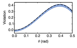
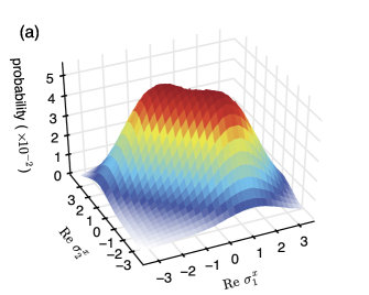
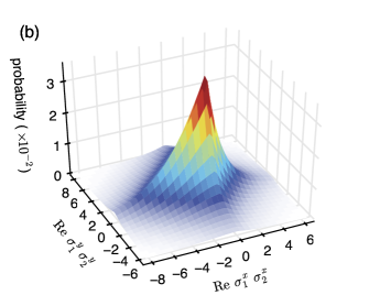
The resulting Bell violation is graphed in Fig (1). This demonstrates complete agreement with quantum predictions, up to a sampling error which can be reduced at will by taking more samples. However, the results of Fig (2) are more interesting. This figure shows the joint distribution of the Schwinger variables that correspond to the spin projections and their correlations. In a physical measurement, these would all have eigenvalues of . Instead, we see that the variables corresponding to spin measurements go outside their quantum bounds. Intriguingly, this is exactly what is predicted for weak measurements, which suggests that a close relationship exists between these simulations and the concept of a weak measurement.


6 Conclusions
Our main result is that the earliest argument leading to quantum computers is wrong. There is no impediment to simulating Bell violations probabilistically. Our phase-space simulations correctly generate the means and correlations that are predicted by quantum mechanics. Such probabilistic simulation methods have already allowed simulations of the quantum dynamics of quantum solitons [10, 11] and colliding Bose-Einstein condensates [12], with up to modes and particles. The growth of sampling error and other scaling issues are important limitations, and will be treated elsewhere.
Quantum logic based encryption [13] and atomic clocks [14] are already successful. To develop such technologies in future [15], understanding the consequences of non-ideal behavior is very important. Probabilistic algorithms could therefore have an application to the design of these devices. Importantly, fundamental tests of quantum mechanics require simulation methods that do not depend on quantum theory being correct, which is a strong reason to investigate these issues further.
References
References
- [1] Feynman R P 1982 Int. J. Theor. Phys. 21 467–488
- [2] Husimi K 1940 Proc. Phys. Math. Soc. Jpn. 22 264–314 URL https://www.jstage.jst.go.jp/article/ppmsj1919/22/4/22_4_264/_pdf
- [3] Drummond P D and Gardiner C W 1980 J. Phys. A: Math. Gen. 13 2353–2368
- [4] Bennett C H 2000 IBM J. Res. Dev. 44 270–277 ISSN 0018-8646 URL http://dx.doi.org/10.1147/rd.441.0270
- [5] Bell J S 1964 Physics 1 195–200 URL http://philoscience.unibe.ch/documents/TexteHS10/bell1964epr.pdf
- [6] Clauser J F, Horne M, Shimony A and Holt R 1969 Phys. Rev. Lett. 23 880–884
- [7] Drummond P D 1983 Phys. Rev. Lett. 50 1407–1410
- [8] Reid M D and Walls D F 1986 Phys. Rev. A 34(2) 1260–1276 URL http://link.aps.org/doi/10.1103/PhysRevA.34.1260
- [9] McNeil K J and Gardiner C W 1983 Phys. Rev. A 28(3) 1560–1566 URL http://link.aps.org/doi/10.1103/PhysRevA.28.1560
- [10] Carter S J, Drummond P D, Reid M D and Shelby R M 1987 Phys. Rev. Lett. 58(18) 1841–1844
- [11] Corney J F, Drummond P D, Heersink J, Josse V, Leuchs G and Andersen U L 2006 Phys. Rev. Lett. 97(2) 023606
- [12] Deuar P and Drummond P D 2007 Phys. Rev. Lett. 98 120402
- [13] Bennett C H, Brassard G and Mermin N D 1992 Phys. Rev. Lett. 68(5) 557–559 URL http://link.aps.org/doi/10.1103/PhysRevLett.68.557
- [14] Chou C W, Hume D B, Koelemeij J C J, Wineland D J and Rosenband T 2010 Phys. Rev. Lett. 104(7) 070802 URL http://link.aps.org/doi/10.1103/PhysRevLett.104.070802
- [15] Jones N C, Van Meter R, Fowler A G, McMahon P L, Kim J, Ladd T D and Yamamoto Y 2012 Phys. Rev. X 2(3) 031007 URL http://link.aps.org/doi/10.1103/PhysRevX.2.031007