Three-body forces from a classical nonlinear field

Abstract

Forces in the systems of two opposite sign and three identical charges coupled to the dynamical scalar field of the signum-Gordon model are investigated. Three-body force is present, and the exact formula for it is found. Flipping the sign of one of the two charges changes not only the sign but also the magnitude of the force. Both effects are due to nonlinearity of the field equation.

PACS: 11.27.+d, 11.10.Lm, 03.50.Kk

1 Introduction

As is well-known, relativistic scalar fields play the crucial roles in physics of fundamental interactions from particle physics to cosmology. Topological and non-topological solitons [1], [2], long lived oscillons [3], phenomena such as spontaneous symmetry breaking and Higgs mechanism [4], all can hardly be considered without scalar fields. Not surprisingly, one can find in literature a whole variety of field-theoretic models with scalar fields. We have been interested in the so called signum-Gordon model which involves just one classical scalar field $\varphi$, real or complex. Its defining feature is the V-shaped self-interaction potential proportional to the modulus of the field, $U(\varphi)=g|\varphi|$, where $g>0$ is the self-coupling constant. This model originated from investigations of perturbations of the ground state of a system of harmonically coupled pendulums bouncing from a stiff rod in the constant gravitational field [5]. It has turned out that it has truly amazing properties. Its basic dynamical features, which do not depend on the dimension of space-time, include a scale invariance of the on-shell type, and generically a very fast, parabolic approach of the field to its ground state value $\varphi=0$, which is reached exactly on a finite distance. Because of the latter property, the signum-Gordon field may formally be regarded as an ultramassive one, because the massless or massive fields have a different asymptotic behavior of Coulomb or Yukawa type, respectively.

Furthermore, in the case of real signum-Gordon field the field equation has the form

$$\partial_{\mu}\partial^{\mu}\varphi=-g\>\mbox{sign}\>\varphi,$$ (1)

where the sign function has the standard values $\pm 1$ and $\mbox{sign}\>0=0$. Thus, the r.h.s. of this equation is piecewise constant, greatly facilitating construction of interesting analytic solutions. In fact, its solutions include non-radiating oscillons [6], as well as a whole family of self-similar fields [7]. In the case of complex scalar field with the V-shaped self-interaction compact Q-balls were found [8]. In all these cases pertinent exact analytic solutions were obtained. Thus the signum-Gordon model has turned out to be a very good theoretical laboratory for studying the highly nontrivial, nonlinear dynamics of scalar fields.

Recently, we have investigated forces exerted on static external charges interacting with the real signum-Gordon field [9]. In particular, the force $F_{qq}(a)$ between two identical, separated by the distance $a$, point static charges of the strength $q$ has been calculated. It exactly vanishes when the distance between the charges exceeds certain finite value $a_{*}$ that depends on their strengths. Such unusual behavior is due to the fact that $U^{\prime}=g\>\mbox{sign}\>\varphi$ remains finite even for arbitrarily small values of the field $\varphi$. This is similar to the constant gravity force attracting a ball to floor. The scalar field forms a compact cloud surrounding the charges. The force is attractive.

In the present paper we extend the work [9] by presenting two effects that are due to nonlinearity of the signum-Gordon field. The point is that in the case of one-dimensional space one can construct the exact solutions of the inhomogeneous signum-Gordon equation (Eq. (4) below) for any number of static, point-like external sources. This gives us the rare opportunity of having full knowledge about the effects that are due to the self-interaction of the signum-Gordon field – the mediating field for the forces between the external charges. Specifically, we consider the force $F_{-qq}(a)$ between two opposite static charges $-q$ and $q$ separated by the distance $a$, and the forces in the system of three identical static charges. We obtain exact formulas for the scalar mediating field and for the forces. In the $-qq$ case, the field and force vanish when the distance $a$ exceeds the same finite value $a_{*}$ as in the $qq$ system investigated in [9]. The force is repulsive, as expected. Our new finding is that the magnitudes of the forces in the $qq$ and $-qq$ cases are different, $|F_{-qq}(a)|\neq|F_{q}(a)|$, as opposed to the case of charges coupled to a free field, e.g., electric charges interacting with the electromagnetic field. Our most interesting result however is the observation that in the case of three charges a three-body force is present. It is clear that in general one should expect $N$-body forces when there are $N$ charges. These effects are due to the nonlinearity of field equation and therefore are expected to appear in other nonlinear field-theoretic models.

The plan of our paper is as follows. In the next section we briefly recall the method of calculating the forces, we explain how one can obtain the pertinent solution of field equation, and we discuss the $-qq$ case. The three-body forces in the $qqq$ case are calculated in Section 3. Summary and remarks are collected in Section 4.

2 The force in the $-qq$ case

We consider two static, point-like charges of the opposite sign interacting with the dynamical real scalar field $\varphi$ . The Lagrangian for this system has the form (we use the $c=\hbar=1$ units)

$$L=\frac{1}{2}\partial_{\mu}\varphi\partial^{\mu}\varphi-g\>|\varphi|+j\varphi,$$ (2)

where

$$j(x)=q\>\delta(x-a)-q\>\delta(x).$$ (3)

Here $\mu=0,1$, and $x\equiv x^{1}$ is the spatial coordinate in the one-dimensional space. The charges are located at $x=0$ and $x=a>0$. The field equation corresponding to this Lagrangian reads

$$\partial_{\mu}\partial^{\mu}\varphi+g\>\mbox{sign}\>\varphi=j(x).$$ (4)

The simplest way to obtain the $\mbox{sign}\>\varphi$ term is first to regularize the field potential, e.g., $\>g\>|\varphi|\rightarrow g\>\sqrt{\delta^{2}+\varphi^{2}}$, and to take the limit $\delta\rightarrow 0$ in the term $g\>\varphi/\sqrt{\delta^{2}+\varphi^{2}}$ that appears in the corresponding Euler-Lagrange equation. Thus,

$$\mbox{sign}\>\varphi=\lim_{\delta\rightarrow 0}\frac{\varphi}{\sqrt{\delta^{2}+\varphi^{2}}}.$$

It is clear from this definition that $\mbox{sign}\>0=0$. Such regularized version of the signum-Gordon model, i.e., with $\delta>0$, was investigated on its own right in [10].

The force exerted on the charge $-q$ located at $x=0$ is given by the total flux of momentum towards that charge, as explained in, e.g., [11], [9]. The momentum density and the flux of momentum are given by the energy-momentum tensor of our system,

$$T_{\mu\nu}=\partial_{\mu}\varphi\partial_{\nu}\varphi-\eta_{\mu\nu}L,$$ (5)

where $(\eta_{\mu\nu})=\mbox{diag}(1,-1)$ is the Minkowski metric.

The total momentum $P^{1}$ of the field, given by

$$P^{1}=-\int dx\>T_{01}=-\int dx\>\partial_{0}\varphi\>\partial_{x}\varphi,$$

vanishes in the case of static fields we consider. The presence of the point charges breaks the translational symmetry. In consequence, instead of the continuity equation $\partial^{\mu}T_{\mu\nu}=0$ we have

$$\partial^{\mu}T_{\mu\nu}=-\varphi\partial_{\nu}j.$$ (6)

The flux of momentum along the $x$ axis is given by $T_{11}=(\partial_{x}\varphi)^{2}/2-g\>|\varphi|$ if $x\neq 0,a$. By the definition, the force exerted on the charge located at $x=0$ is given by the rate at which the momentum is transferred to that charge. Hence,

$$F^{1}=\left.T_{11}\right|_{x=-\epsilon}-\left.T_{11}\right|_{x=\epsilon}.$$ (7)

Here $\epsilon$ can be any number from the interval $(0,a)$, because in the static case the identity (6) implies that $T_{11}$ does not depend on $x$ in the open intervals $(-\infty,0)$, $(0,a)$, $(a,\infty)$, in which $j=0$. Furthermore, we will see that the pertinent solution $\varphi$ and $T_{11}$ vanish in the interval $(-\infty,-d_{0})$, where $d_{0}>0$ is a constant. Therefore, $\left.T_{11}\right|_{x=-\epsilon}=0$, and formula (7) is simplified to

$$F^{1}=-\left.T_{11}\right|_{x=\epsilon}.$$ (8)

It remains to find the field $\varphi$ in the presence of the sources. In the static case it satisfies the equation

$$\partial^{2}_{x}\varphi-g\>\mbox{sign}\>\varphi=q\delta(x)-q\delta(x-a).$$ (9)

In order to ensure finiteness of the total energy $E=\int dx\>T_{00}$, where $T_{00}=(\partial_{x}\varphi)^{2}/2+g\>|\varphi|$, the field $\varphi$ and $\partial_{x}\varphi$ should vanish for $|x|\rightarrow\infty$. Furthermore, integrating both sides of Eq. (9) over intervals of the half-length $\delta<a$ around $x=0$ and $x=a$ we obtain the conditions

$$\partial_{x}\varphi(\delta)-\partial_{x}\varphi(-\delta)=q,\;\;\;\;\partial_{x}\varphi(a+\delta)-\partial_{x}\varphi(a-\delta)=-q,$$ (10)

which are the one-dimensional counterpart of Gauss law of electrostatics. These conditions imply that $\partial_{x}\varphi$ is discontinuous at the locations of the charges.

Obvious approach to solving Eq. (9) is first to find solutions of the homogeneous equation

$$\partial^{2}_{x}\varphi-g\>\mbox{sign}\>\varphi=0$$ (11)

in the open intervals $(-\infty,0),$ $(0,a)$ and $(a,\infty)$. Next, we glue them at $x=0$, $x=a$, so that $\varphi$ is continuous function of $x$ at these points, and that the conditions (10), in which we may take the limit $\delta\rightarrow 0+$, are satisfied.

The general solution of Eq. (11) in the interval in which $\varphi>0$, i.e., $\mbox{sign}\>\varphi=+1$, has the form

$$\varphi(x)=\frac{g}{2}x^{2}+Ax+B,$$ (12)

and if $\mbox{sign}\>\varphi=-1$ then

$$\varphi(x)=-\frac{g}{2}x^{2}+Cx+D,$$ (13)

where $A,B,C,D$ are constants to be determined from the matching conditions. There also exists the trivial solution $\varphi=0$ which represents the ground state of the classical signum-Gordon field. Our Ansatz for the solution has the following form

$$\varphi_{-qq}(x)=\left\{\begin{array}[]{ll}0&\;\;\;x\leq-d_{0},\\ u_{1}(x)&\;\;\;x\in[-d_{0},0],\\ u_{2}(x)&\;\;\;x\in[0,d_{1}],\\ u_{3}(x)&\;\;\;x\in[d_{1},a],\\ u_{4}(x)&\;\;\;x\in[a,a+d_{2}],\\ 0&\;\;\;x\geq a+d_{2},\end{array}\right.$$ (14)

where $d_{0}>0$, $d_{2}>0$, $d_{1}\in(0,a)$ are constants to be determined. The functions $u_{1},u_{2}$ are negative inside their domains and have the form (13), while $u_{3},u_{4}$ are positive and have the form (12), see Fig. 1.

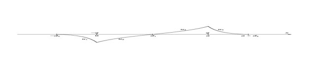
Figure 1: Schematic picture of the nontrivial part of the solution (14) for the $-qq$ case

The function $u_{1}$ matches the ground state solution $\varphi=0$ at the point $x=-d_{0}$. The matching conditions are the continuity of $\varphi$ and $\partial_{x}\varphi$. Trivial calculation gives

$$u_{1}(x)=-\frac{g}{2}\left(x+d_{0}\right)^{2}.$$ (15)

The function $u_{2}$ obeys the conditions

$$u_{2}(0)=u_{1}(0),\;\;\;\partial_{x}u_{2}(0)-\partial_{x}u_{1}(0)=q,\;\;\;u_{2}(d_{1})=0.$$

Simple calculations give

$$u_{2}(x)=-\frac{g}{2}(d_{1}-x)\left(\frac{d_{0}^{2}}{d_{1}}-x\right),$$ (16)

and the relation

$$(d_{0}+d_{1})^{2}=\frac{2q}{g}d_{1}.$$ (17)

The function $u_{4}$ has the general form (12) with the coefficients $A,B$ determined from the conditions $u_{4}(a+d_{2})=0$, $\>\partial_{x}u_{4}(a+d_{2})=0$, which ensure the correct matching of $u_{4}$ with the trivial solution $\varphi=0$ at the point $x=a+d_{2}$. It turns out that

$$u_{4}(x)=\frac{g}{2}\left(x-a-d_{2}\right)^{2}.$$ (18)

The function $u_{3}$ of the general form (12) has to obey four conditions: the matching conditions with the function $u_{2}$ at the point $x=d_{1}$, i.e., $u_{3}(d_{1})=0$, $\partial_{x}u_{2}(d_{1})=\partial_{x}u_{3}(d_{1})$, and the conditions $u_{3}(a)=u_{4}(a)$, $\partial_{x}u_{3}(a)-\partial_{x}u_{4}(a)=q$ at the point $x=a$. These conditions determine the precise form of $u_{3}$, namely

$$u_{3}(x)=\frac{g}{2}(x-d_{1})\left(x-2d_{1}+\frac{d_{0}^{2}}{d_{1}}\right),$$ (19)

and also give the following relations

$$(d_{2}+a-d_{1})^{2}=\frac{2q}{g}(a-d_{1}),\;\;\;\;2d_{1}+d_{0}=a+d_{2}.$$ (20)

These relations together with (17) fix the constants $d_{0},d_{1},d_{2}$:

$$d_{0}=d_{2}=\sqrt{\frac{qa}{g}}-\frac{a}{2},\;\;\;\;d_{1}=\frac{a}{2}.$$ (21)

The force exerted on the charge $-q$ located at $x=0$ is given by formula (8), in which we put $T_{11}|_{x=\epsilon}=(\partial_{x}u_{2}(0))^{2}/2-gu_{2}(0)$. Simple calculation gives

$$F_{-qq}^{1}(a)=-\frac{1}{2}q^{2}\left(1-\sqrt{\frac{a}{a_{*}}}\right)^{2},$$ (22)

where

$$a_{*}=\frac{q}{g}.$$

We see that the force is repulsive one. It contains the one-dimensional scalar Coulomb force $F^{1}_{Coul}=-q^{2}/2$ as the leading term when $a\ll a_{*}$.

The solution (14) and formula (22) for the force are valid when $a\in(0,a_{*}]$. When the distance $a$ between the charges is equal to $a_{*}$ the charges become completely screened by the scalar field. When $a>a_{*}$, each charge is surrounded by a compact cloud of the field of the width $a_{*}$. The clouds do not overlap – in between them there is the region with the ground state field $\varphi=0$. Thus the charges do not feel the presence of each other, and the force vanishes of course. Such screening has been observed already in [9] in the case of two identical point-like charges $qq$ located at $x=0$ and $x=a$. In this case the force exerted on the charge located at $x=0$ is given by the following formula

$$F^{1}_{qq}(a)=\frac{1}{2}q^{2}\left(1-\frac{a}{a_{*}}\right).$$ (23)

Apart from the difference in sign, which means that $F^{1}_{qq}(a)$ is an attractive force, we see different dependence on the distance $a$. Because this difference disappears when we put the coupling constant $g=0$, it is related to the presence of the nonlinear $\mbox{sign}\>\varphi$ term in the field equation (4).

3 The three-body forces

Let us now consider three identical point charges of the strength $q$ located at the points $x=-a$, $x=0$ and $x=b$, where $a,b>0$. In this case Eq. (4) takes the form

$$\partial^{2}_{x}\varphi-g\>\mbox{sign}\>\varphi=q\delta(x+a)+q\delta(x)+q\delta(x-b).$$ (24)

The Ansatz for the solution has the form

$$\varphi_{qqq}(x)=\left\{\begin{array}[]{ll}0&\;\;\;x\leq-a-d_{-},\\ w_{1}(x)&\;\;\;x\in[-a-d_{-},-a],\\ w_{2}(x)&\;\;\;x\in[-a,0],\\ w_{3}(x)&\;\;\;x\in[0,b],\\ w_{4}(x)&\;\;\;x\in[b,b+d_{+}],\\ 0&\;\;\;x\geq b+d_{+},\end{array}\right.$$ (25)

where $d_{+},d_{-}>0$ are constants. All functions $w_{i}(x)$, $i=1,..,4$, are strictly positive inside their domains, so they have the general form (12). The nontrivial part of the function $\varphi_{qqq}(x)$ is depicted in Fig. 2.

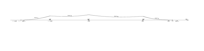
Figure 2: Schematic picture of the nontrivial part of the solution (25) for the case of three identical charges

The constants in these functions and the constants $d_{\pm}$ are determined from the matching conditions which ensure continuity of $\varphi_{qqq}$ everywhere and continuity of $\partial_{x}\varphi_{qqq}$ at $x=-a-d_{-}$, $x=b+d_{+}$, and from the ‘Gauss law’ relations of the type (10) at $x=-a$, $x=0$, $x=b$. Because the pertinent calculations are straightforward and completely analogous to the ones presented in the -qq case, we just quote the results:

$$w_{1}(x)=\frac{1}{2}\>g\left(x+a+d_{-}\right)^{2},$$ (26)

$$w_{2}(x)=\frac{1}{2}\>g\left(x+a+d_{-}\right)^{2}-q(x+a),$$ (27)

$$w_{3}(x)=\frac{1}{2}\>g\left(x-b-d_{+}\right)^{2}+q(x-b),$$ (28)

$$w_{4}(x)=\frac{1}{2}\>g\left(x-b-d_{+}\right)^{2},$$ (29)

where

$$d_{-}=\frac{3}{2}\>a_{*}-\frac{1}{3}\>b-\frac{2}{3}\>a,\;\;\;d_{+}=\frac{3}{2}\>a_{*}-\frac{2}{3}\>b-\frac{1}{3}\>a.$$ (30)

The solution (25) is correct provided that $a$ and $b$ are not too large, otherwise one charge (or more) will be completely screened by the compact cloud of the scalar field, as discussed in [9]. Such a screened charge decouples from the others. In such cases, in between the clouds there are segments of the $x$ axis where the field has its ground state value $\varphi=0$, and the force on such a distant charge exactly vanishes. More precisely, for the validity of the solution (25) $a$ and $b$ should satisfy the following bounds

$$2a+b<3a_{*},\;\;\;\;a+2b<3a_{*}.$$ (31)

The decoupling of the charge located at $x=-a$ from the two other occurs when $a=3a_{*}/2-b/2$. This can be found by checking when the function $w_{2}$ has a zero in the interval $(-a,0)$. If $w_{2}<0$ in that interval, the function (25) ceases to be the solution of Eq. (24). The decoupling of the charge located at $x=b$ takes place when $b=3a_{*}/2-a/2$. In this case one should check positivity of the $w_{3}$ function.

It is clear from the considerations at the beginning of Section 2 that the total force exerted on the charge located at $x=-a$ is given by the formula

$$F_{-a}=-\left.T_{11}(w_{2})\right|_{x=-a}=q^{2}\left(1-\frac{2a+b}{3a_{*}}\right).$$ (32)

This force is the attractive one.

Let us compare this force with the sum of two-body forces exerted on this charge by the charges located at $x=0$ and $x=b$. For the two-body forces we use formula (23) assuming that $a<a_{*}$, $a+b<a_{*}$, so that our charge is in the interaction range of the two other charges. We obtain

$$F_{2body}(-a)=q^{2}\left(1-\frac{2a+b}{2a_{*}}\right).$$

The difference

$$F_{3body}(-a)=F_{-a}-F_{2body}(-a)=q^{2}\frac{2a+b}{6a_{*}}$$

gives the three-body component of the total force exerted on that charge. This component is negligibly small if $a\ll a_{*}$, $b\ll a_{*}$ (when the constant scalar Coulomb force dominates), but it cannot be neglected if the distances between the charges become comparable with $a_{*}$.

The force exerted on the charge located at $x=0$ also has a three-body component. The total force is calculated from the formula

$$F_{0}=\left.T_{11}(w_{2})\right|_{x=0}-\left.T_{11}(w_{3})\right|_{x=0}=q^{2}\frac{a-b}{3a_{*}}.$$

On the other hand, the sum of two-body forces exerted by the neighboring charges is equal to

$$F_{2body}(0)=q^{2}\frac{a-b}{2a_{*}}.$$

Here we assume that $a,b\ll a_{*}$, so that the use of formula (23) is formally justified. Again, the three-body component ,

$$F_{3body}(0)=F_{0}-F_{2body}(0)=q^{2}\frac{b-a}{6a_{*}},$$

can have a sizable magnitude.

The force exerted on the charge located at $x=b$ is given by the formula

$$F_{b}=\left.T_{11}(w_{3})\right|_{x=b}=-q^{2}\left(1-\frac{a+2b}{3a_{*}}\right).$$

It differs from the force $F_{-a}$ by the sign, and $a$ and $b$ are interchanged, as expected in view of the spatial structure of our $qqq$ system.

4 Summary and remarks

1. We have found the exact form of the scalar field in the presence of two and three point-like external charges in one dimensional space. For simplicity, we have considered the $-qq$ and $qqq$ systems, but a generalization to charges of arbitrary strength is straightforward. The fields have the parabolic, compact tails that are characteristic for models with the V-shaped self-interactions. Next, we have calculated the forces exerted on the charges. Our main finding is that the forces are shaped mainly by the self-coupling of the mediating field. Only at the very short distances ($a\ll a_{*}$) the familiar scalar Coulomb force dominates, and the self-interaction of the field is not important.

2. Particularly interesting is the presence of the three-body force. Generalizing our result, we expect that in a system of $N$ particles coupled to a non-linear field all $n$-body forces will appear with $n=2,3,\ldots N$. We have seen that the three-body force can have a significant strength. This would cast a shadow on attempts to model dynamics of many particle systems by Hamiltonians that include only two-particle interactions. The importance of the many-body forces has recently been emphasized in, e.g., [12] in the context of nuclear physics, and in [13] in condensed matter physics.

3. It is clear that nonlinear field-theoretic effects in interactions of systems of many particles are in general present and important. As a good illustration of this point one may take the results presented in [14], where an explanation of rotation curves of galaxies without invoking the concept of dark matter is proposed. It would be very interesting to investigate the many-body forces in the case of particles coupled to a non-Abelian gauge field of the $SU(n)$ type.

References

- [1] T. Vachaspati, Kinks and Domain Walls. An Introduction to Classical and Quantum Solitons. Cambridge University Press, Cambridge, 2006.
- [2] L. Wilets, Nontopological Solitons. World Scientific, Singapore, 1989.
- [3] See, e.g., I. L. Bogolyubskii and V. G. Makhankov, Sov. Phys. JETP Lett. 24, 12 (1976); M. Gleiser, Phys. Rev. D 49, 2978 (1994); M. Gleiser and D. Sicilia, Phys. Rev. Lett. 101, 011602 (2008).
- [4] See, e.g., S. Weinberg, The Quantum Theory of Fields. Vol. II Modern Applications. Cambridge University Press, Cambridge, 1996. Chapters 19, 21.
- [5] H. Arodź, Acta Phys. Polon. B 35, 625 (2004).
- [6] H. Arodź and Z. Świerczyński, Phys. Rev. D 84, 067701 (2011).
- [7] H. Arodź, J. Karkowski and Z. Świerczyński, Acta Phys. Polon. B 43, 79 (2012).
- [8] H. Arodź and J. Lis, Phys. Rev. D 79, 045002 (2009).
- [9] H. Arodź, J. Karkowski and Z. Świerczyński, Phys. Rev. D 87, 125004 (2013).
- [10] J. Lis, Acta Phys. Polon. B 41, 629 (2010).
- [11] D. J. Griffiths, Introduction to Electrodynamics. Prentice-Hall, Inc., Upper Saddle River, New Jersey, 1981. Section 8.2.
- [12] See, e.g., A. Cipollone, C. Barbieri and P. Navrátil, Phys. Rev. Lett. 111, 062501 (2013).
- [13] See, e.g., K. A. H. Sellin and E. Babaev, preprint arXiv:1308.2109 [cond-mat.soft].
- [14] J. D. Carrick and F. I. Cooperstock, Astrophys. Space Sci. 337, 321 (2012).