Determination of Acceleration Mechanism Characteristics Directly and Non-Parametrically from Observations: Application to Supernova Remnants

Abstract

We have developed an inversion method for determination of the characteristics of the acceleration mechanism directly and non-parametrically from observations, in contrast to the usual forward fitting of parametric model variables to observations. In two recent papers Petrosian and Chen (2010); Chen and Petrosian (2013), we demonstrate the efficacy of this inversion method by its application to acceleration of electrons in solar flares based on stochastic acceleration by turbulence. Here we explore its application for determining the characteristics of shock acceleration in supernova remnants (SNRs) based on the electron spectra deduced from the observed nonthermal radiation from SNRs and the spectrum of the cosmic ray electrons observed near the Earth. These spectra are related by the process of escape of the electrons from SNRs and energy loss during their transport in the galaxy. Thus, these observations allow us to determine spectral characteristics of the momentum and pitch angle diffusion coefficients, which play crucial roles in both direct acceleration by turbulence and in high Mach number shocks. Assuming that the average electron spectrum deduced from a few well known SNRs is representative of those in the solar neighborhood we find interesting discrepancies between our deduced forms for these coefficients and those expected from well known wave-particle interactions. This may indicate that the standard assumptions made in treatment of shock acceleration need revision. In particular, the escape of particles from SNRs may be more complex than generally assumed.

I Introduction

Acceleration of charge particles in the universe happens on scales from planetary magnetospheres to clusters of galaxies and at energies ranging from nonrelativistic values to $>$10¹⁹ eV ultra high energy cosmic rays (UHECRs). The particles are observed directly as cosmic rays (CRs), solar energetic particles, or indirectly by their interactions with background matter and electromagnetic fields (magnetic fields and photons), which give rise to heating and ionization of the plasma, and nonthermal radiation extending from long wavelength radio to $>$TeV gamma-rays. In spite of more than a century of observations, the exact mechanism of acceleration is still being debated and the detailed model parameters are poorly constrained. Clearly electric fields are involved in any acceleration mechanism. Large scale electric fields have been found to be important in some unusual astrophysical sources such as magnetospheres of neutron stars (pulsars and perhaps magnetars) and in so-called double-layers. However, here we are interested in commonly considered mechanisms based on the original Fermi process Fermi (1949), which involves scattering of particles by fluctuating electric and magnetic fields (or plasma turbulence) or converging flows as in shocks.

The usual approach of determining the acceleration model and its characteristics is to use the forward fitting (FF) method, whereby the model particle spectra based on an assumed mechanism and some parametric form of its characteristics are fitted to observations. For radiating sources, FF is carried out in two stages, first fitting the photon spectra to an assumed radiation mechanism from a parametrized particle spectrum, then fitting the latter to the acceleration model. This approach, even though one can never be certain of the uniqueness of the results, has been fairly successful, and for some observations, e.g., those with poorly determined spatially unresolved spectra, is the best one can do. But in sources with richer observations one can do better.

In this paper we present a new approach which allows a non-parametric determination of acceleration parameters, mainly their energy dependence, irrespective of some of the details of the acceleration mechanism, directly from the observed radiation or otherwise deduced particle spectra. This is done by the inversion of the kinetic differential equations describing the particle acceleration and transport. In our first paper on this subject Petrosian and Chen (2010), we applied this technique to inversion of hard X-ray images of solar flares from the Reuven Ramaty High Energy Solar Spectroscopic Imager (RHESSI) and determined the energy dependence of the escape time from the acceleration region and from it the energy dependence of the rate of scattering of the particles, presumably due to plasma turbulence, which is related to the pitch angle diffusion coefficient $D_{\mu\mu}$, where $\mu$ is the cosine of the pitch angle. In a more recent paper Chen and Petrosian (2013), we have shown that from the same data we can also determine the energy diffusion coefficient $D_{\rm EE}$, which is related to the momentum diffusion coefficient $D_{pp}$. In both papers we formulated this in the framework of stochastic acceleration (SA) by plasma waves or turbulence, which is same as the original Fermi process, nowadays referred to as second-order Fermi acceleration process. Here we extend this approach to simultaneous determination of the scattering and acceleration rates, which depend primarily on $D_{\mu\mu}$ and $D_{pp}$, to situations where both SA by turbulence and acceleration by a shock play important roles. As in previous papers we carry this out in the framework of the so called leaky box model. In the next section we present the kinetic equation describing both acceleration processes, and in §III we describe the process of the inversion and the required data for it. In §IV we describe possible application of this method to the acceleration of electrons in supernova remnants (SNRs). Interpretation and discussions of the results are shown in §V and a brief summary is presented in §VI.

II Kinetic Equations and the Leaky Box Model

The discussion below is a brief summary of this subject given in a recent review by Petrosian (2012) describing the conditions under which the so-called leaky-box model is a good approximation. As emphasized in this review, and recognized by the community at large, it is clear now that plasma waves or turbulence play an essential role in the acceleration of charged particles in a variety of magnetized astrophysical and space environments. Turbulence is expected to be produced by large scale flows in most astrophysical situations because of the prevailing large Reynolds numbers. Once generated on a scale $L$ comparable to the size of the source it undergoes dissipationless cascade from large to small spatial scales, or from small wave numbers $k_{\rm min}\sim 2\pi/L$ up to the dissipation scale given by $k_{\rm max}$, generally with a power law energy density distribution $W(k)\propto k^{-q}$. Resonant interactions between particles and small amplitude electromagnetic fluctuations of turbulence cause diffusion of particles in the phase space. For magnetized plasmas this process can be described by the Fokker-Planck (FP) kinetic equation for gyro-phase averaged, four dimensional (4-D) particle distribution function $f(t,\mu,p,s)$, where $s$ is the distance along the magnetic field lines. This equation involves, in addition to $D_{\mu\mu}$ and $D_{pp}$, a third coefficient $D_{\mu p}=D_{p\mu}$, as well as a source term ${\dot{\cal S}}(t,\mu,p,s)$ and energy losses or gains due to interactions of particles with background plasma (with density $n$, temperature $T$, magnetic field $B$ and soft photon energy density $u_{\rm ph}$). These interactions cause stochastic acceleration, e.g., Sturrock (1966); Schlickeiser (1989), in which particles systematically gain energy with a rate that is proportional to the square of the wave-to-particle velocity ratio as in the second-order Fermi process.

Also shown in Schlickeiser (1989), the 4-D differential equation can be reduced to a 3-D equation, when the scattering time $\tau_{\rm sc}\,\sim 1/D_{\mu\mu}$ is shorter than the dynamic time $\tau_{\rm dyn}$ and the crossing time $\tau_{\rm cross}\,\sim L/v$. Then the momentum distribution is nearly isotropic and one can define the pitch angle averaged quantities, $F(t,p,s)=\frac{1}{2}\int_{-1}^{+1}f(t,\mu,p,s)d\mu$ and ${\dot{S}}(t,p,s)=\frac{1}{2}\int_{-1}^{+1}{\dot{\cal S}}(t,\mu,p,s)d\mu$, and use three pitch angle-averaged transport coefficients

$$\kappa_{ss} = (v/2)^{2}\langle(1-\mu^{2})^{2}/D_{\mu\mu}\rangle\,,$$ (1)

$$\kappa_{sp} = v/(2p)\langle(1-\mu^{2})D_{\mu p}/D_{\mu\mu}\rangle\,,$$ (2)

$$\kappa_{pp} = \langle D{pp}-D^{2}_{\mu p}/D_{\mu\mu}\rangle/p^{2}\,.$$ (3)

(see Petrosian (2012)) to describe spatial and momentum diffusion rates. Schlickeiser (1989) and others, in most subsequent applications of this equation, were interested in acceleration by Alfvén waves (with velocity $v_{A}$), in which case the diffusion coefficients are related as $D_{\mu\mu}:D_{\mu p}/p:D_{pp}/p^{2}=1:(v_{A}/v):(v_{A}/v)^{2}$. Limiting their analysis to low magnetization and high energy particles, i.e. for $v_{A}/v\ll 1$ they used the inequities $D_{\mu\mu}\gg D_{\mu p}/p\gg D_{pp}/p^{2}$ to obtain the simplified equation. However, as was pointed out by Pryadko and Petrosian (1997), at low energies and for strong magnetic fields, other plasma waves become more important than the Alfvén waves and these inequalities are no longer valid, e.g., Dung and Petrosian (1994). Pryadko and Petrosian (1997) suggested another approximation for the FP equation for the opposite limit, $D_{pp}/p^{2}\gg D_{\mu p/p}\gg D_{\mu\mu}$, in which case the momentum diffusion is the dominant term. These ideas were further developed by Petrosian and Liu (2004) and summarized in Petrosian (2012). It turns out that if again $\tau_{\rm sc}\,\ll\tau_{\rm cross}\,$ and $\tau_{\rm dyn}$, then this situation can be described by the same 3-D equation with slightly different coefficients. (The proof of this assertion will be presented elsewhere.)

Finally a second simplification can be used for both cases if the acceleration region is homogeneous, or if one deals with a spatially unresolved acceleration region where one is interested in spatially integrated equations. In this case it is convenient to define the 2-D distribution function in terms of the particle energy $E$, $N(t,E)dE=\int dV[4\pi p^{2}F(t,s,p)dp]$ and ${\dot{Q}}_{\rm inj}(t,E)dE=\int dV[4\pi p^{2}{\dot{S}}(t,s,p)dp]$, introduce spatially averaged terms ${\bar{X}}=\int X(s)F(s)ds/\int F(s)ds$ and replace the spatial diffusion term by an escape term. Then we obtain the following well known equation, sometimes referred to as the leaky box model,

$${\partial N\over\partial t}= {\partial\over\partial E}\left[D_{\rm EE}{\partial N\over\partial E}\right]-{\partial\over\partial E}\left[(A(E)-\dot{E}_{\rm L})N\right]$$

$$-{N\over T_{\rm esc}}+{\dot{Q}}_{\rm inj}\,,$$ (4)

where $D_{\rm EE}=v^{2}p^{2}\bar{\kappa}_{pp}$, $A(E)$ and $\dot{E}_{\rm L}$ are the direct acceleration and energy loss rates, and ${\dot{Q}}_{\rm inj}(t,E)$ and $N(t,E)/T_{\rm esc}$ represent the rates of injection and escape of particles in and out of the whole acceleration site. For purely SA, the direct acceleration rate

$$A_{\rm SA}(E)=2{\bar{\xi}}D_{\rm EE}/E=2\xi^{\prime}E\bar{\kappa}_{pp},$$ (5)

where

$${\bar{\xi}}={\gamma^{2}-0.5\over\gamma^{2}+\gamma}\,\,\,\,{\rm and}\,\,\,\,\,\xi^{\prime}=\frac{(\gamma+1)(2\gamma^{2}-1)}{2\gamma^{3}}.$$ (6)

The term $\xi^{\prime}$ is nearly equal to 1 at all $\gamma$ (it has a maximum of $\sim$1.3 for $\gamma\sim 1.8$).

Because the acceleration rate in stochastic acceleration is proportional to the square of the velocity ratio $v_{A}/v$, it is often regarded to be too slow to account for production of high-energy particles, especially in comparison to acceleration in a shock (or a converging flow in general). For a shock with velocity $u_{\rm sh}$, a particle of velocity $v$ upon crossing it gains momentum linearly with velocity; $\delta p=p(u_{\rm sh}/v)$, and therefore this often is referred to as a first-order Fermi process. There are several misconceptions associated with the above statement. The first is that the diffusion coefficients, in general, increase with decreasing particle energy so that SA can be very efficient in the acceleration of low energy particles in the background plasma, which is where all acceleration processes must start Hamilton and Petrosian (1992); Dung and Petrosian (1994). The second is that shock acceleration is not related to the original first-order Fermi process Fermi (1954), and the third is that shock acceleration rate is also second order.

In an unmagnetized shock, or in a shock with magnetic field parallel to the shock velocity, acceleration requires an scattering agent to recycle particles repeatedly across the shock. Turbulence is the most likely agent for this. The acceleration rate then is $\delta p/\delta t$, where the recycling time $\delta t\sim{\bar{\kappa}}_{ss}/(vu_{\rm sh})$ Krymsky et al. (1979); Lagage and Cesarsky (1983); Drury (1983); Dröge and Schlickeiser (1986). Thus, the shock acceleration rate, $A^{\|}_{\rm sh}\propto Eu_{\rm sh}^{2}/{\bar{\kappa}}_{ss}\propto E(u_{\rm sh}/v)^{2}\langle(1-\mu^{2})^{2}/D_{\mu\mu}\rangle$, is also a second order mechanism. As shown by Jokipii (1987), for oblique shocks ($\theta>0$) the acceleration rate also varies as the square of shock velocity, but in this case, specifically for a perpendicular shock ($\theta=\pi/2$) the rate could be much higher. In general then, as emphasized in Petrosian (2012), in both SA by turbulence and shock acceleration the rates are proportional to the square of the velocity ratios $u_{\rm sh}/v$ and $v_{\rm A}/v$, respectively, so that the distinction between them is greatly blurred. In either process, resonant scattering by turbulence provides rapid isotropization of the particle pitch angle distribution, a necessary prerequisite for efficient acceleration, e.g., Melrose (2009).

More exactly, in the framework of the leaky box model, the shock acceleration rate can be written as

$$A_{\rm sh}=E\left(1+\frac{1}{\gamma}\right)\left(\frac{u_{\rm sh}^{2}}{\bar{\kappa}_{ss}}\right)\zeta f(\theta,\eta),$$ (7)

where we have introduced the parameter $\zeta=(r-1)/(3r)$ with $r$ the compression ratio and $f(\theta,\eta)$ which is a somewhat complicated function of the angle and the ratio of the diffusion coefficients parallel to perpendicular to the magnetic field $\eta=k_{\|}/k_{\perp}$; Steinacker et al. (1988); Jokipii (1987); Dröge and Schlickeiser (1986). For a parallel shock $f=1$ and ${\bar{\kappa}}_{ss}=\kappa_{1}+r\kappa_{2}$, where subscript 1 and 2 refer to upstream and downstream region of the shock, respectively. The usual practice is to assume the Bohm limit; $\kappa\propto vr_{g}/3$, where $r_{g}=v/\Omega$ is the gyro radius. In what follows we will use a more accurate relation for ${\bar{\kappa}}_{ss}$ obtained from wave particle interactions, as those shown in Figure (1). For a perpendicular shock the relation again is simple and from Jokipii (1987) we obtain ${\bar{\kappa}_{ss}}/f(\pi/2,\eta)=2\eta\kappa_{ss}/(1+\eta^{2})\sim 2\kappa_{ss}/\eta$ (for $\eta\gg 1$), which amounts to setting $f(\theta=\pi/2,\eta)=\eta$.

In applications to astrophysical sources we will be dealing with the scattering and stochastic acceleration times defined as as

$$\tau_{\rm sc}\,(E)=3{\bar{\kappa}_{ss}\over v^{2}}=\frac{3}{4}\langle(1-\mu^{2})^{2}/{\bar{D}}_{\mu\mu}\rangle,$$ (8)

$$\tau_{\rm ac}\,(E)=\bar{\kappa}_{pp}^{-1}={p^{2}\over\langle{{\bar{D}}_{pp}-{\bar{D}}^{2}_{p\mu}/{\bar{D}}_{\mu\mu}}\rangle},$$ (9)

Using these in Eqs. (5) and (7) we can write shock to SA acceleration rate ratio as

$$\frac{A_{\rm sh}}{A_{\rm SA}}=2\left(\frac{u_{\rm sh}}{v}\right)^{2}\left(\frac{\tau_{\rm ac}\,}{\tau_{\rm sc}\,}\right)\zeta\xi^{\prime\prime}f,$$ (10)

where $\xi^{\prime\prime}=\gamma^{2}/(\gamma^{2}-0.5)$. For parallel shocks ($f=1$) this ratio becomes $A_{\rm sh}/A_{\rm SA}\sim(\tau_{\rm ac}\,/\tau_{\rm sc}\,))(u_{\rm sh}/v)^{2}$. As pointed out above (and in Pryadko and Petrosian (1997)), at low energies and for strong magnetic fields, $\tau_{\rm ac}\,/\tau_{\rm sc}\,<1$ indicating the dominance of SA. But for high energies and Alfvénic turbulence $\tau_{\rm ac}\,/\tau_{\rm sc}\,\sim(v/v_{A})^{2}$ and $A_{\rm sh}/A_{\rm SA}\sim{\cal M}_{A}^{2}$, where ${\cal M}_{A}=u_{\rm sh}/v_{A}$ is the Alfvén Mach number, so shock acceleration dominates at high energies and weakly magnetized plasmas. Figure 1 shows a comparison between the SA timescale $\tau_{\rm ac}\,$ as defined in Eq. (9) and shock acceleration time $\tau_{\rm ac,sh}=E/A_{\rm sh}\sim(v/u_{\rm sh})^{2}\tau_{\rm sc}\,$, based on rates obtained for interactions of electrons with parallel propagating plasma waves Pryadko and Petrosian (1997), for two values of the spectral index $q$ of the turbulence energy density and two degrees of magnetization described by the plasma parameter $\alpha=3.2\times 10^{3}\sqrt{n/{\rm cm}^{-3}}(\mu{\rm G}/B)$, which is equal to the ratio of the electron plasma to gyro frequencies. As evident at low energies and small values of $\alpha$ (strong magnetization) SA is the dominant mechanism. For oblique shocks the shock rate will be in general higher by some factor which depends on the angle $\theta$; e.g. for a high Mach number ($r=4,\zeta=1/4$) perpendicular ($\theta=\pi/2$) shock this factor will be $\sim\eta/2$.

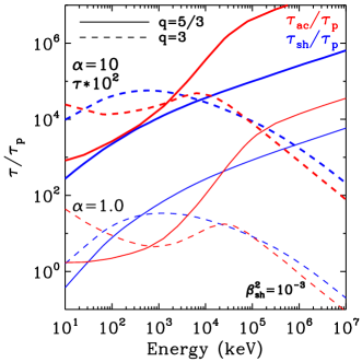
Figure 1: Comparison of the SA time (denote here as $\tau_{\rm ac}$) calculated using Eq. (9) and shock acceleration time (denoted here as $\tau_{\rm sh}\equiv E/A_{\rm sh}$) for interactions of electrons with parallel propagating plasma waves with power law spectral distribution for two indicies $q=5/3$ (Kolmogorov) and 3. Here $\alpha=3.2\times 10^{3}\sqrt{n/{\rm cm}^{-3}}(\mu{\rm G}/B)$, the ratio of the electron plasma to gyro frequencies, is a measure of the degree of magnetization, and $\tau_{p}^{-1}\propto\Omega f_{\rm turb}$ is the characteristic rate for wave-particle interactions. (See more details in Pryadko and Petrosian (1997); Petrosian and Liu (2004).) Note that for highly magnetized plasma ($\alpha=1.0)$, SA is the dominant mechanism at some energies, and even for a plasma with lower magnetization, SA cannot be ignored. The shock velocity is taken to be $u_{\rm sh}=10^{4}$ km/s compared to the Alfvén velocity $v_{A}=c/[(m_{p}/m_{e})^{1/2}\alpha]\sim 7000$ and 700 km/s, resulting in ${\cal M}^{2}_{A}=2$ and 200, respectively. The proportionality constants $\zeta$ and $f$ are set to unity. Note that the $q=5/3$ solid curves are multiplied by 100 for clarity.

In Petrosian (2012) it was suggested that in presence of a shock the acceleration may be a hybrid process dominated by SA at low energies and shock at high energies. In what follows we will consider the combined processes, which depend on wave-particle interactions, shock compression ratio and background plasma parameters.

For a solution of the differential Eq. (II) we also need the energy dependence of the other terms. For the injected spectrum ${\dot{Q}}_{\rm inj}(E)$ we will consider a Maxwellian distribution at a given temperature $kT\ll m_{e}c^{2}$, and for the energy loss we include ionization and Coulomb losses that dominate at low energies (and depend on background density $n$ and ionic composition), and synchrotron and inverse Compton losses that dominate at high energies (and depend on the background magnetic field and photon energy densities). Coulomb interactions can also cause energy and pitch angle diffusion which become important at low energies, e.g., McTiernan and Petrosian (1990); Petrosian and East (2008).

As we will see below the last term, namely the escape time, is the term that can be obtained most readily from observations, which then allows determination of the other terms. However, the relation of the escape time to the coefficients of the acceleration mechanism is complicated. As shown in Petrosian (2012), it is related to an integral of spatial diffusion term $\kappa_{ss}$ over the acceleration site. Thus, it also depends on the size $L$ of this site or crossing time $\tau_{\rm cross}\,=L/v$. For the isotropic case with $\tau_{\rm sc}\,\ll\tau_{\rm cross}\,$, one expect the diffusion of the particles across the source to follow a random walk process, which means we can write $T_{\rm esc}\sim\tau^{2}_{\rm cross}/\tau_{\rm sc}\,$. In the opposite limit, $\tau_{\rm cross}\,\ll\tau_{\rm sc}\,$, the escape time $T_{\rm esc}\sim\tau_{\rm cross}\,$. Combining these two cases in the past we (Petrosian and Liu (2004)) have used the approximate expression

$$T_{\rm esc}=\tau_{\rm cross}\,(1+\tau_{\rm cross}\,/\tau_{\rm sc}\,).$$ (11)

However, other geometric effects such as those produced by the large scale magnetic fields e.g. chaotic field lines, or strongly converging or diverging field configurations (see Chen and Petrosian (2013)), or deviation from isotropy or a simple spherical homogeneous acceleration site, can make the relation between $T_{\rm esc}$ and other acceleration coefficients more complex.

III The Inversion Process

III.1 The Knowns and Unknowns

Solution of Eq. (II) requires knowledge of energy and time dependences of the five coefficients involved in the terms on the right side. In situations where there exist time resolved observations one needs to solve for the time dependence of the accelerated spectrum. However, if the dynamic time $\tau_{\rm dyn}$ describing the evolution is longer than the characteristic timescales associated with these coefficients (such as $\tau_{\rm sc}\,,\tau_{\rm cross}\,$ and $\tau_{\rm ac}\,$ or energy diffusion time $\tau_{\rm diff}\sim E^{2}/D_{\rm EE}$), then one can use the steady state assumption and set ${\partial N\over\partial t}=0$ and modulate the results with the time profile of the dynamic process. This was the case in our application of the inversion method to solar flares. In the opposite situation of short dynamic time, and in the absence of temporally resolved observations, one can integrate Eq. (II) over the dynamic time in which case $\int_{0}^{\infty}{\partial N\over\partial t}dt=0$, because we expect $N(t=\infty,E)=N(t=0,E)=0$ for high energy particles. In this case one is dealing with the values of the coefficients averaged over duration $\Delta t$ of the process; e.g average injected spectrum ${\dot{\bar{Q}}}(E)=\int_{\Delta t}{\dot{Q}}(t,E)dt/\Delta t$. As discussed below this will be the case for the application to SNRs and cosmic ray electrons (CRes). Thus, we need to consider only the energy dependence of the coefficients.

Two of these, namely $\dot{E}_{\rm L}$ and ${\dot{Q}}_{\rm inj}$, depend on background plasma parameters $n,T,B$ and $u_{\rm ph}$, and are independent of the acceleration process. We will assume that we have sufficient information on the background plasma so that we know the values and energy dependences of these two terms. The other three are related to the characteristics of the acceleration mechanism that we want to determine. One of these is the energy diffusion coefficient $D_{\rm EE}$ (related to $D_{pp}$). The escape time depends on the size $L$ of the source and on the spatial diffusion rate (related $D_{\mu\mu}$). The final term, namely the direct acceleration rate has contribution from turbulence, which is related to $D_{\rm EE}$, and from shocks, which is related to $D_{\mu\mu}$ and the characteristics of the shocks described above. Assuming that we know the value of the latter and the size $L$ of the acceleration site, we are left with two primary unknowns $D_{\mu\mu}$ and $D_{pp}$, or in terms of more directly unknowns $D_{\rm EE}$ and $T_{\rm esc}$. Therefore, in order to determine the energy dependences of these two coefficients, we need the variation with energy of two independent observed quantities, as described next.

III.2 Escape Time

As described in Petrosian and Chen (2010), one of the two functions that observations can provide is the (spatially integrated) energy spectrum of the accelerated particles $N(E)$, which can be deduced from the observed total photon spectrum $I(\epsilon)$ produced in the acceleration region. If the escape time is finite then the rate of particles escaping will be ${\dot{Q}}_{\rm esc}=N/T_{\rm esc}$. If this spectrum is measured directly, we then can obtain the escape time simply as

$$T_{\rm esc}(E)=N(E)/{\dot{Q}}_{\rm esc}(E).$$ (12)

If we assume that Eq. (11) is an accurate description of how particles escape, we can then obtain also the scattering time

$$\tau_{\rm sc}\,=\frac{\tau_{\rm cross}^{2}}{N(E)/{\dot{Q}}_{\rm esc}(E)-\tau_{\rm cross}\,}.$$ (13)

This will then give a measure of the pitch angle diffusion coefficients $D_{\mu\mu}$ and as shown by Eqs.(7) and (9), it will also give the acceleration rate by the shock $A_{\rm sh}(E)$, assuming we know $\zeta$.

III.3 Energy Diffusion and Acceleration Rates

Given the above information we are left with only two related unknowns, namely the energy diffusion coefficient $D_{\rm EE}$ or the direct SA rate $A_{\rm SA}=2{\bar{\xi}}D_{\rm EE}/E$. This final unknown can be obtained using our knowledge of the accelerated particle spectra $N(E)$ and the escape time $T_{\rm esc}(E)$ by the inversion of the leaky box Eq. (II) as follows.

The key aspect here is to recognize that this ordinary differential equation is only first-order in the derivative of $D_{\rm EE}$ with respect to $E$, instead of second-order that appears to be the case in its alternate form. Thus, by utilizing the relation between $A_{\rm SA}$ and $D_{\rm EE}$ in Eq. (5) we can rewrite the steady state leaky box equation as

$$\frac{d}{dE}\left[D_{\rm EE}\frac{N}{E}\left(\frac{d\ln{N}}{d\ln{E}}-\xi\right)\right]+\frac{d}{dE}\left[(\dot{E}_{\rm L}-A_{\rm sh})N\right]$$

$$=\frac{N}{T_{\rm esc}}-{\dot{Q}}_{\rm inj},$$ (14)

Integrating this from $E$ to $\infty$ gives

$$D_{\rm EE}=E\left[\dot{E}_{\rm L}-A_{\rm sh}+\frac{1}{N}\int_{E}^{\infty}\left(\frac{N}{T_{\rm esc}}-{\dot{Q}}_{\rm inj}\right)dE\right]$$

$$\times\left(2{\bar{\xi}}-\frac{d\ln{N}}{d\ln{E}}\right)^{-1},$$ (15)

from which we obtain $A_{\rm SA}=2{\bar{\xi}}D_{\rm EE}/E$. Thus, all the terms on the right-hand side can in principle be obtained directly from observables.

Note that for the time integrated equation under consideration here we must have the equality $\int_{0}^{\infty}{\dot{Q}}_{\rm inj}(E)dE=\int_{0}^{\infty}N(E)/T_{\rm esc}(E)dE$. But for relevant energies of $E\gg kT$ only a number of particles in the Maxwellian tail contribute and ${\dot{Q}}_{\rm inj}\ll N(E)/T_{\rm esc}(E)$. If this were not true there would be very few particles accelerated and the case is uninteresting. Thus, in what follows we can neglect the injection term. However, given the temperature of the background particles this term can be easily calculated and included in the results.

Finally we define an effective acceleration rate as

$$A_{\rm eff}\equiv A_{\rm sh}+A_{\rm SA}\eta_{\rm acc}=\dot{E}_{\rm L}+\frac{1}{N}\int_{E}^{\infty}\frac{N}{T_{\rm esc}}dE,$$ (16)

where $\eta_{\rm acc}\equiv 1+\delta_{\rm acc}/(2{\bar{\xi}})$, and we have introduced the spectral index of the accelerated particles $\delta_{\rm acc}=-d\ln{N}/d\ln{E}$. At relativistic energies ${\bar{\xi}}\rightarrow 1$ and, as we will see below, typically $\delta_{\rm acc}\sim 2$, so this rate is sum of the shock and (about two times) SA rates.

III.4 Escaping Particles

Escaping particle are measured directly or by the detection of the radiation they produce outside the acceleration site, which we will call the transport region, where their spectrum is modified due to transport effects. These effects can be treated by a similar kinetic equation without the diffusion and acceleration terms. If the particles are injected into a finite region and if one can neglect further acceleration and assume that pitch angle scattering quickly isotropizes the particle distribution, then the evolution of particles in the transport region can be described by the leaky box Eq. (II) which now has only the energy loss and escape terms. Instead of a thermal background source term, the spectrum of particles injected in the transport region is same as those escaping the acceleration site;

$${\dot{Q}}^{\rm tr}_{\rm inj}(E)={\dot{Q}}_{\rm esc}(E)=\frac{N_{\rm acc}(E)}{T_{\rm esc}^{\rm acc}(E)}.$$ (17)

In application to the transport of the CRs in the galaxy we are dealing with a long dynamic time so that we can use the steady state equation, which has the formal solution giving the effective spectrum of particles integrated over the transport region Stawarz et al. (2010),

$$N_{\rm eff}(E)={\tau_{\rm L}^{\rm tr}(E)\over E}\,\int_{E}^{\infty}dE^{\prime}\,\,{\dot{Q}}^{\rm tr}_{\rm inj}(E^{\prime})$$

$$\times\exp\left[-\int_{E}^{E^{\prime}}{dE^{\prime\prime}\over E^{\prime\prime}}\,\,{\tau_{\rm L}^{\rm tr}(E^{\prime\prime})\over T_{\rm esc}^{\rm tr}(E^{\prime\prime})}\right]\,,$$ (18)

where we have defined the energy loss time $\tau^{\rm tr}_{\rm L}\equiv E/{\dot{E}}^{\rm tr}_{\rm L}$.

Of special importance, in general and in particular for the applications described below, is the case when the particles escaping the acceleration site lose all their energy in the transport region. This is referred to as the thick target or totally cooled spectral model, where one sets $T_{\rm esc}^{\rm tr}=\infty$ and get a simpler integral solution

$$N_{\rm eff}(E) =\frac{\tau_{\rm L}^{\rm tr}}{E}\int_{E}^{\infty}dE^{\prime}{\dot{Q}}^{\rm tr}_{\rm inj}(E^{\prime})$$

$$=\frac{\tau_{\rm L}^{\rm tr}}{E}\int_{E}^{\infty}dE^{\prime}\frac{N_{\rm acc}(E^{\prime})}{T_{\rm esc}^{\rm acc}(E^{\prime})}.$$ (19)

First, differentiating this equation we derive the desired expression for the escape time as

$$T_{\rm esc}^{\rm acc}(E)={\tau_{\rm L}^{\rm tr}}\left[\frac{N_{\rm acc}}{N_{\rm eff}}\right]\eta_{\rm eff}^{-1},$$ (20)

where $\eta_{\rm eff}\equiv\delta_{\rm eff}+\frac{d\ln{\tau}^{\rm tr}_{\rm L}}{d\ln E}-1$, and we have defined the spectral index $\delta_{\rm eff}=-d\ln N_{\rm eff}/d\ln E$. Second, we note that this last integrand is identical to the third term inside the square brackets on the right-hand side of Eq. (III.3), so that with the help of this equation we can derive a new simpler relation for the energy diffusion rate as

$$D_{\rm EE}={E^{2}}\left(\frac{1}{\tau_{\rm L}^{\rm acc}}-{A_{\rm sh}\over E}+\frac{N_{\rm eff}}{\tau_{\rm L}^{\rm tr}N_{\rm acc}}\right)(2{\bar{\xi}}+\delta_{\rm acc})^{-1},$$ (21)

where $\tau^{\rm acc}_{\rm L}\equiv E/{\dot{E}}_{\rm L}$ is the energy loss time scale averaged over the acceleration region. Finally, we define the effective acceleration time (a combination of shock and SA times)

$$\tau_{\rm ac,eff}(E)\equiv\frac{E}{A_{\rm eff}} =\left[{1\over\tau_{\rm L}^{\rm acc}}+{1\over\tau_{\rm L}^{\rm tr}}{N_{\rm eff}\over N_{\rm acc}}\right]^{-1}$$

$$=\left[{1\over\tau_{\rm L}^{\rm acc}}+{1\over\eta_{\rm eff}T_{\rm esc}}\right]^{-1}.$$ (22)

For pure shock acceleration, the acceleration time $\tau_{\rm ac,sh}=\tau_{\rm ac,eff}$ and for pure SA, the time $\tau_{\rm ac,SA}=\tau_{\rm ac,eff}\eta_{\rm acc}$. Note that while the escape time depends on only the ratio of effective to acceleration spectra, the acceleration times involve both this ratio and the energy loss time in the acceleration site.

In the opposite limit when particles lose very little of their energy in the transport region, i.e. when $T_{\rm esc}^{\rm tr}\ll\tau_{\rm L}^{\rm tr}$, which is called the thin target model, Eq. (III.4) simplifies even further to

$$N_{\rm eff}(E)=T_{\rm esc}^{\rm tr}(E){\dot{Q}}^{\rm tr}_{\rm inj}(E)=\frac{T_{\rm esc}^{\rm tr}(E)}{T_{\rm esc}^{\rm acc}(E)}N_{\rm acc}(E),$$ (23)

from which we get

$$T_{\rm esc}^{\rm acc}(E)=T_{\rm esc}^{\rm tr}(E)[N_{\rm acc}/N_{\rm eff}].$$ (24)

For the diffusion coefficient in this case we have to replace the last term inside the first pairs of parenthesis on the right-hand side of Eq. (21) by $\int_{E}^{\infty}(N_{\rm eff}/T_{\rm esc}^{\rm tr})dE/N_{\rm acc}$. In what follows we will consider only the thick target case.

In summary, the above equations show that one can determine the pitch angle and momentum diffusion coefficients in the acceleration region directly from measurements of the particle spectra in the acceleration and transport regions.

As mentioned at the outset, in Chen and Petrosian (2013) we have demonstrated the power of the procedure in application to solar flares. Here we explore the possibility of using the radiative signatures of SNRs and observed spectra of CRes in the interstellar medium (ISM) to determine the characteristics of the acceleration mechanism in SNRs.

IV Applications to Supernova Remnants

It has been the common belief that SNRs are the source of the observed CRs (at least up to the knee at $\sim$10¹⁵ eV) and recent high energy gamma-ray observations of SNRs have enforced this belief considerably. If this is true then we can get information on the two functions required for our inversion process. The observed radiative spectrum of SNRs from radio to gamma-rays gives the spectrum of the the accelerated particles, $N_{\rm acc}(E)$, and the observed spectrum of the CRs provides information on the spectrum of accelerated particles escaping the SNRs, $N_{\rm eff}(E)$. Although in principle this information is available for both electrons and protons, there are only some preliminary solid observations on the radiative signature of protons in SNRs. Therefore, in what follows we will focus on the acceleration of electrons.

However, it should be emphasized that the situation here is not as straightforward as in solar flares where these two functions are determined simultaneously for individual flares. Here we need knowledge of the transport to the Earth of the electrons escaping the SNRs, and a more important complexity is that, many and a diverse set of SNRs, resulting from explosions of different progenitor stars in different environments, contribute to the CRs in the ISM. We will address these complexities in the following sections.

IV.1 Spectrum of Accelerated Electrons in SNRs

Many SNRs are observed optically and at radio. The radio radiation produced via the synchrotron mechanism provides the original indication of presence of electrons with energy $E>$ GeV in a magnetic field of $B_{\rm snr}\sim$ 10–20 $\mu$G. Several SNRs are detected at X-rays which also are attributed to synchrotron radiation by more energetic electrons, perhaps in a stronger magnetic field. Fermi and HESS have detected GeV and TeV gamma-rays in several SNRs. In some cases, for example SNR RXJ1713.7–3946, a pure leptonic scenario, whereby the gamma-rays are produced by the synchrotron emitting electrons via the inverse Compton (IC) scattering of cosmic microwave background (CMB) or other soft photons, seems to work Li et al. (2011). While in others, e.g., SNR Tycho Giordano et al. (2012), the hadronic scenario, whereby the accelerated protons are responsible for the gamma-rays, fits the data better. In some others, e.g., SNR Vela Jr. Tanaka et al. (2011), both models give acceptable fits. In any case the radio and X-ray emission gives information about the spectrum of the accelerated electrons which is what we will be concerned with here. We call this spectrum $N^{\rm snr}_{\rm acc}(E)$.

In the case of solar flares, where nonthermal electron bremsstrahlung produces the hard X-ray radiation, one can use regularized inversion procedures to determine the spectrum of the radiating electrons non-parametrically and directly from photon count spectra Petrosian and Chen (2010). Unfortunately this technique cannot be used for SNRs. There has not been much effort in inverting synchrotron and IC spectra to obtain electron spectra non-parametrically. Some time ago, Brown et al. (1983) addressed the inversion of synchrotron spectra and recently Li et al. (2011) used a matrix inversion method of Johns and Lin (1992) to invert the IC spectra and applied it to SNR RXJ1713.7–3946. But, in general, most of the information on $N_{\rm acc}^{\rm snr}$ is obtained by FF of the observed photon spectra to parametric electron spectra, with the result that the accelerated electron spectra (integrated over the acceleration region of SNR) can be described by a power low with a high energy exponential cut off at energy $E_{\rm snr}$. Here and in what follows we express all particle energies in units of a fiducial energy $E_{0}$, which we set equal to 100 GeV for numerical purposes. Thus, the spectrum of SNR can be written as

$$N_{\rm acc}^{\rm snr}(E)dE=N^{\rm snr}_{0}f(E/E_{0})dE/E_{0},$$ (25)

where

$$f(x)=x^{-\alpha_{1}}\exp\left[{-(x/{\rm x_{\rm snr}})^{\alpha_{2}}+(1/x_{\rm snr})^{\alpha_{2}}}\right],$$ (26)

with $x=E/E_{0}$ and $x_{\rm snr}=E_{\rm snr}/E_{0}$. In most cases $\alpha_{1}\sim 2,\,\alpha_{2}\sim 0.5$ and $E_{\rm snr}\sim 6$ TeV provide good fits down to energies of $\sim 2\sqrt{B_{\rm snr}/15\ \mu{\rm G}}$ GeV, e.g., Li et al. (2011); Lazendic et al. (2004). Note that as defined above $f(1)=1$, and $N^{\rm snr}_{0}$ is a dimensionless quantity.

The analyses that lead to the above spectra also indicate presence of sufficiently strong magnetic field ($B_{\rm snr}\geq 15\ \mu$G) that can come about from amplification of the weaker ISM field ($\sim$ 1 $\mu$G) by the supernova driven forward shock. In this case synchrotron losses dominate over IC losses and the radiative loss time in the acceleration site required for our procedure can be written as

$$\tau_{\rm L}^{\rm acc}=\tau_{\rm L,0}^{\rm acc}E_{0}/E,$$ (27)

where

$$\tau_{\rm L,0}^{\rm acc} \equiv\left({6\pi m_{e}c\over\sigma_{T}}\right)\left({m_{e}c^{2}\over E_{0}}\right)B_{\rm snr}^{-2}$$

$$=0.54\times 10^{6}\left({100\ {\rm GeV}\over E_{0}}\right)\left({15\ \mu{\rm G}\over B_{\rm snr}}\right)^{2}{\rm yr},$$ (28)

and $\sigma_{T}$ is the Thomson cross section.

As mentioned above, however, supernova explosions and SNRs may have a broad range of characteristics and parameters of acceleration. In which case the average SNR spectrum contributing to the CRes would depend on the distribution of the spectral parameters, say $\Phi(\alpha_{i},E_{\rm snr})$, where $\alpha_{i}$ stands for $\alpha_{1}$ and $\alpha_{2}$. In this case the average spectral shape

$$\langle f(x)\rangle=\int\int f(\alpha_{i},E_{\rm snr};x)\Phi(\alpha_{i},E_{\rm snr})d\alpha_{i}dE_{\rm snr}$$ (29)

will depend on the shape of the distribution $\Phi$. As we will see below only the value of $\alpha_{1}$ will be important. This is related to the power-law indicies of the observed radio spectra which shows a small dispersion (see Weiler et al. (2010)). In addition, as is well known from general theoretical considerations (Krymskii (1977); Axford et al. (1978); Bell (1978); Blandford and Ostriker (1978)), the power-law index of accelerated particle spectra are insensitive to shock characteristics (e.g. compression ratio) for high Mach number shocks, such as those expected from stellar explosion in the cold ISM. Thus, the spectral shape given in Eq. (26) seems to be a reasonable approximation. It should be noted though that explosions and environments of the upper end main sequence stars are considerably different than those of lower mass stars (see e.g. Prantzos et al. (1986); Woosley et al. (2002)) and could possibly yield different accelerated spectra. Unfortunately there are no observations of remnants of such stars. This is mainly because they are rarer, which would also mean they contribute less to CRs. In addition, explosions into a hot stellar wind environment may lead to a lower Mach number shock and a weaker accelerator. On the other hand, being more powerful explosions could have an opposite effect, which would enhance their contribution.

In the absence of observational evidence about the distribution of characteristics of stellar explosions and SNR spectra, in what follows we will use the spectral form given in Eq. (26) for the accelerated spectrum $N_{\rm acc}(E)$, with the cautionary remark that the above unknown may introduce a significant uncertainty in our final results.

IV.2 Spectrum and Propagation of CR Electrons

As mentioned above, it is widely believed that SNRs are the source of all CRs, and we will assume this to be the case for CRes. Therefore, the spectra of CRs are related to those of the particles emitting the SNR radiation via the escape time from the SNRs. The escaping particles interact with the galactic background matter and electromagnetic fields producing the galactic diffuse emission from radio to high energy gamma-rays. These interactions and other processes modify the escaping particle spectra during their transport to where they radiate and to near the Earth where they are observed directly. Therefore, CRs are expected to have different spectra than SNRs with the difference being partially due to the energy dependence of the escape time and partially due to energy losses during their transport in the galaxy. Observations witness these differences. For example, radio spectra of SNRs are flatter than those of diffuse radio emission in the ISM, and the measured CRe spectrum $J^{\rm CR}_{e}(E)$ is different than that given in Eq. (25). The spectral flux of CRes has been measured by many instruments with varied results. But most recent measurements by Fermi, HESS and PAMELA have produced a very precise spectrum shown in Figure 2. As discussed extensively in the literature these spectra show a well defined deviation from pure power law above 10 GeV and HESS observations provide a clear evidence of a high energy roll over.

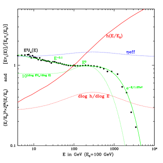
Figure 2: Spectrum of CRes multiplied by $E^{3}$ (dots) as observed by PAMELA (3 lowest energies), HESS (5 highest energies) and Fermi (from Adriani et al. (2011); Aharonian et al. (2008); Ackermann et al. (2010)), respectively. The solid-green curve gives an approximate fit to the observations with its logarithmic derivative shown by the dotted-green curve. We also present a sample variation of $h(E/E_{0})$ (from Stawarz et al. (2010)), the energy loss time (multiplied by $E$; solid-red) and its logarithmic derivative (dotted-red) showing the transition due to the Klein-Nishina effect (see Eq. 32). The dotted-blue curve gives $\eta_{\rm eff}$ defined in Eq. (20) and used in Eq. (49).

There has been multiple analyses of this data. Many of these use GALPROP Moskalenko and Strong (1998) or other similar numerical schemes (e.g., Dragon) to account for transport effects in the galaxy assuming values for background particle and soft photon densities, large scale magnetic field and a spectrum electromagnetic field fluctuations.. This is usually carried out by fitting the observed CRe data to some parametric form of the spectrum of the total electrons injected throughout the galaxy, which is our function ${\dot{Q}}_{\rm inj}^{\rm tr}$ (Eq. 17). The results usually consist of a primary power law component with index $s$ and a high energy exponential cutoff at $E_{\rm CRe}$ so that we have

$${\dot{Q}}_{\rm inj}^{\rm tr}(E)dE={\dot{Q}}_{\rm inj,0}^{\rm tr}g(E/E_{0})dE/E_{0},$$ (30)

where

$$g(x)=x^{-s}e^{-(x-1)/x_{\rm CRe}}\,\,\,\,\,{\rm with}\,\,\,\,\,x_{\rm CRe}=E_{\rm CRe}/E_{0}.$$ (31)

Here ${\dot{Q}}_{\rm inj,0}^{\rm tr}$ is in units of electrons per unit time and $g(1)=1$.

Different analyses give different explanations for the prominent bump seen around 100 GeV. For example, Ackermann et al. (2010) attribute this bump to a flux of electrons (plus positrons) coming from a nearby pulsar yielding $s=2.7$ and $E_{\rm CRe}\sim 2$ TeV. Strong et al. (2011) explain the bump with yet another spectral break, a slight flattening above 50 GeV and similar values for the other parameters. Di Bernardo et al. (2013), using the spectrum of diffuse galactic radio emission, obtain $s\sim 2.5$ but do not have the spectral resolution to see the bump around 100 GeV nor do they see the TeV cutoff. We can use the above expression in Eqs. (17) and (III.4) to obtain the acceleration characteristics. As described below this will be one of the two methods we will use, with $s=2.6$ and $E_{\rm CRe}\sim 2$ TeV.

An alternative and simpler explanation of the bump in the CRe spectrum was given in Stawarz et al. (2010) (see also Schlickeiser and Ruppel (2010)), who show that the energy dependence of radiative losses due to combined synchrotron and IC scattering (by star light, infrared and CMB photons) can account for this deviation. This is because at low energies star light is the dominant agent of loss, but at higher energies IC scattering by star light enters the Klein-Nishina (KN for short) regime which suppresses these losses and there is a transition to IC losses to infrared and CMB photons (which are still in the Thomson regime up to energies of a few TeV) and/or synchrotron losses (depending on the value of the magnetic field). For typical values of the relevant quantities in the solar neighborhood this transition occurs near the bump seen in the CRe spectrum. This means that in this case the radiative loss time that enters Eq. (20) does not have the simple Thomson regime form $\tau_{\rm L}\,\propto E$, but involves an additional function $h(E/E_{0})$ that slowly varies with energy in the range from 1 GeV to 1 TeV shown in Figure 2 (taken from Fig. 1 of Stawarz et al. (2010)). The energy loss time in the transport region can then be written as

$$\tau_{\rm L}^{\rm tr}=\tau_{\rm L,0}^{\rm tr}(E_{0}/E)h(E/E_{0}),$$ (32)

where

$$\tau_{\rm L,0}^{\rm tr}\equiv\left(\frac{6\pi m_{e}c}{\sigma_{T}}\right)\left(\frac{m_{e}c^{2}}{E_{0}}\right)B_{\rm eff}^{-2}.$$ (33)

Here $B_{\rm eff}=\sqrt{8\pi u_{\rm tot}}\sim$ 7 $\mu$G in the solar neighborhood, where $u_{\rm tot}$ is the energy density of all soft photons plus the magnetic field. In this case the observed CRe flux spectrum $J_{e}^{\rm CR}$ gives directly the effective spectrum as

$$N_{\rm eff}(E)dE =4\pi V_{\rm CRe}J^{\rm CR}_{e}(E)dE/c$$

$$\equiv N^{\rm CR}_{0}j(E/E_{0})dE/E_{0},$$ (34)

where $V_{\rm CRe}$ is the volume of the galaxy filled with CRes, $j(1)=1$, and $N^{\rm CR}_{0}=4\pi V_{\rm CR}J^{\rm CR}_{e}(E_{0})/c$ is the (dimensionless) effective total electron number at $E_{0}$. As described below we will use the above two equation, with the exact observed spectrum for $J_{e}^{\rm CR}(E)$, as a second method. It should be noted that here, unlike in the previous method, which assumes presence of nearby pulsar, we assume the solar neighborhood is a typical location in the galaxy, e.g. does not contain an unusual large scale fluctuation in density, $B$ field or turbulence (see also the discussion below).

IV.3 The Two Methods in Practice

We have described two possible methods for inversion of observations to obtain acceleration mechanism characteristics in SNRs. In what follows we discuss how these methods work in practice.

The SNR spectrum $N_{\rm acc}^{\rm snr}(E)$, and either the deduced injected CRe spectrum ${\dot{Q}}_{\rm inj}^{\rm tr}$ or the observed CRe spectrum $J_{e}^{\rm CR}(E)$ provide the energy dependence of the two functions $N(E)$ and $N_{\rm eff}(E)$ that we need for our analysis but not their normalization which is required for determining their ratio. We have already discussed the uncertainty in the spectrum $N_{\rm acc}^{\rm snr}(E)$ above. Here we describe the uncertainty in the normalizations. This normalization depends not only on $N^{\rm snr}_{0},{\dot{Q}}_{\rm inj,0}^{\rm tr}$ and $N^{\rm CR}_{0}$, but also on the rate of SNR formation per unit volume ${\dot{n}}_{\rm snr}({\bf r},t)$. Given this rate we can determine the averaged density of accelerated electrons in the galaxy and the rate of injection of electrons per unit volume in the ISM as

$$n_{\rm acc}(E,t)\equiv N_{\rm acc}(E,t)/V_{\rm snr}$$

$$=\frac{1}{V_{\rm snr}}\int_{V_{\rm snr}}d^{3}{\bf r}\int_{0}^{t}{\dot{n}}_{\rm snr}({\bf r},t_{b})N^{\rm snr}_{\rm acc}(E,{\bf r},t-t_{b})dt_{b},$$ (35)

and

$${\dot{q}}^{\rm tr}_{\rm inj}(E,t)\equiv{\dot{Q}}^{\rm tr}_{\rm inj}(E,t)/V_{\rm CRe}$$

$$=\frac{1}{V_{\rm CRe}}\int_{V_{\rm snr}}d^{3}{\bf r}\int_{0}^{t}{\dot{n}}_{\rm snr}({\bf r},t_{b}){N^{\rm snr}_{\rm acc}(E,{\bf r},t-t_{b})\over T_{\rm esc}^{\rm acc}(E,{\bf r},t-t_{b})}dt_{b},$$ (36)

where $t_{b}$ is the birth time of SNRs, and $V_{\rm snr}$, the volume of the galaxy enclosing all SNRs is expected to be or less than $V_{\rm CRe}$. However this difference does not affect our results.

In general, the integrands vary in time and space, but because the active age of a SNR, $\tau_{\rm snr}$, is much shorter than other ages, in particular the age of the galaxy, only the SNR formation rate averaged over the past $\tau_{\rm snr}$ years enters these equations. Moreover, because electrons in several GeV to TeV range lose their energy quickly, only the quantities within the finite volume of radius $R\sim\sqrt{3\tau_{\rm L}^{\rm tr}/\tau_{\rm sc}^{\rm tr}}\lambda_{{\rm sc}}^{\rm tr}\sim 1$ kpc around the solar neighborhood are relevant (here $\lambda_{{\rm sc}}^{\rm tr}=v\tau_{\rm sc}^{\rm tr}\sim 2$ pc at 100 GeV is the scattering mean free path of CRes in the ISM). Then the injection rate is determined by the value of the integrand of the above equations averaged over a small volume and short time $t_{0}-\tau_{\rm snr}<t<t_{0}$ or nearly for $t\simeq t_{0}$, the current age of the galaxy. Thus, we can write

$$N_{\rm acc}(E,t_{0})=N_{{\rm acc},0}f(E/E_{0})/E_{0},$$ (37)

where

$$N_{{\rm acc},0}\equiv N_{0}^{\rm snr}[V_{\rm snr}{\dot{n}}_{\rm snr}(t_{0})\tau_{\rm snr}],$$ (38)

and

$${\dot{Q}}_{\rm inj}^{\rm tr}(E,t_{0})=N_{\rm acc}(E,t_{0})/T^{\rm acc}_{\rm esc}(E,t_{0}).$$ (39)

In what follows we suppress the time $t_{0}$.

These results assume that $f(E/E_{0})$ is the electron spectrum integrated or averaged over the active life of the SNRs. And as stressed above, because the number of accelerated electrons may vary from SNR to SNR, the normalization constants also stand for averaged quantities. For example, given the distribution function ${\dot{\Psi}}(N^{\rm snr})$ the integrand in Eq. (IV.3) is ${\dot{n}}_{\rm snr}N^{\rm snr}=\int_{0}^{\infty}N^{\rm snr}{\dot{\Psi}}(N^{\rm snr})dN^{\rm snr}$.

Method A: In this method we use the deduced injected spectrum as given by Eq. (30). Equating this observed spectrum to that in Eq. (39) we obtain the escape time (from SNRs) as

$$T^{\rm acc}_{\rm esc}(E)=T_{{\rm esc},0}[f(E/E_{0})/g(E/E_{0})],$$ (40)

with

$$T_{{\rm esc},0}=N_{{\rm acc},0}/{\dot{Q}}_{\rm inj,0}^{\rm tr},$$ (41)

and the effective spectrum as

$$N_{\rm eff} =(\tau_{\rm L}^{\rm tr}/E){\dot{Q}}_{\rm inj,0}^{\rm tr}\int_{E}^{\infty}g(E/E_{0})dE/E_{0}$$

$$=(\tau_{\rm L}^{\rm tr}/E_{0}){\dot{Q}}_{\rm inj,0}^{\rm tr}{\tilde{g}}(E/E_{0}).$$ (42)

Here we have defined ${\tilde{g}}(x)=\int_{x}^{\infty}g(x^{\prime})dx^{\prime}]/x=g(x)/\eta_{g}$, where $\eta_{g}\sim(x/x_{\rm CRe}+s-0.5)$. As shown in Eqs. (21) and (III.4) the diffusion coefficient and effective acceleration time depend only on the following combination of terms

$${N_{\rm eff}\over\tau_{\rm L}^{\rm tr}N_{\rm acc}}={1\over T_{{\rm esc},0}}{g(E/E_{0})\over\eta_{g}f(E/E_{0})},$$ (43)

and, in particular, the effective acceleration time is obtained as

$$\tau_{\rm ac,eff}(E)=\tau_{\rm L}^{\rm acc}\left[1+{\tau_{\rm L}^{\rm acc}\over T_{{\rm esc},0}}{g(E/E_{0})\over\eta_{g}f(E/E_{0})}\right]^{-1}.$$ (44)

We can lump all the unknown and poorly known factors that enter in these equations into a single parameter

$${\cal R}_{a}=\frac{T_{{\rm esc},0}}{\tau_{\rm L,0}^{\rm acc}}=\frac{N_{0}^{\rm snr}[V_{\rm snr}{\dot{n}}_{\rm snr}(t_{0})\tau_{\rm snr}]}{\tau_{\rm L,0}^{\rm acc}{\dot{Q}}_{\rm inj,0}^{\rm tr}},$$ (45)

which then gives

$$T^{\rm acc}_{\rm esc}(E)=\tau_{\rm L,0}^{\rm acc}\left[{\cal R}_{a}{f(E/E_{0})\over g(E/E_{0})}\right]\eta_{\rm eff}^{-1},$$ (46)

and

$$\tau_{\rm ac,eff}=\tau_{\rm L,0}^{\rm acc}\left[{E\over E_{0}}+{\cal R}_{a}^{-1}{g(E/E_{0})\over\eta_{g}f(E/E_{0})}\right]^{-1}.$$ (47)

Thus, both timescales $T^{\rm acc}_{\rm esc}(E)$ and $\tau_{\rm ac,eff}(E)$ can be expressed in units of $\tau_{\rm L,0}^{\rm acc}$ (which depends only on the average magnetic field in the acceleration region), and their values and the energy dependence of $\tau_{\rm ac,eff}(E)$ vary with the value of the parameter ${\cal R}_{a}$. Note that in this method the (more uncertain) energy loss rate in the ISM does not enter into these results. Its effect is included in deducing the injected spectrum from the observed CRe spectrum. In other words, given the magnetic field in the SNR acceleration region around the shock the spectra depend only on ${\cal R}_{a}$ (or $T_{\rm esc,0}$), which involves the properties of the SNRs and the normalization of the deduced injected electrons.

Method B: Alternatively, as mentioned above, we can get the effective spectrum directly from the observed CRe spectrum as $N_{\rm eff}=N^{\rm CR}_{0}j(E/E_{0})/E_{0}$, in which case instead of Eq. (43) we have

$${N_{\rm eff}\over N_{\rm acc}}={N^{\rm CR}_{0}\over N_{\rm acc,0}}{j(E/E_{0})\over f(E/E_{0})},$$ (48)

which when substituted into Eqs. (20) and (III.4) gives the unknown escape and effective acceleration times as

$$T_{\rm esc}={\tau_{\rm L,0}^{\rm acc}\over\eta_{\rm eff}}\left[{\cal R}_{b}{f(E/E_{0})h(E/E_{0})\over(E/E_{0})j(E/E_{0})}\right]\eta_{\rm eff},$$ (49)

with

$$\eta_{\rm eff}=-d\ln j/d\ln E+d\ln h/d\ln E-2,$$ (50)

and

$$\tau_{\rm ac,eff}=\tau_{\rm L,0}^{\rm acc}\left[{E\over E_{0}}+{\cal R}_{b}^{-1}{(E/E_{0})j(E/E_{0})\over h(E/E_{0})f(E/E_{0})}\right]^{-1},$$ (51)

where we have defined

$${\cal R}_{b}\equiv{\tau_{\rm L,0}^{\rm tr}N_{\rm acc,0}\over\tau_{\rm L,0}^{\rm acc}N^{\rm CR}_{0}}={V_{\rm snr}[N_{0}^{\rm snr}{\dot{n}}_{\rm snr}(t_{0})\tau_{\rm snr}]\over N_{0}^{\rm CR}}\left({B_{\rm snr}\over B_{\rm eff}}\right)^{2}.$$ (52)

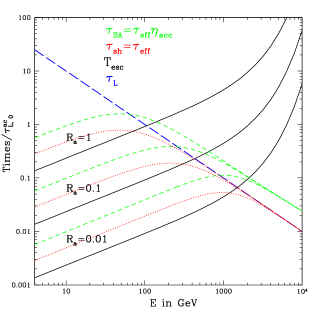
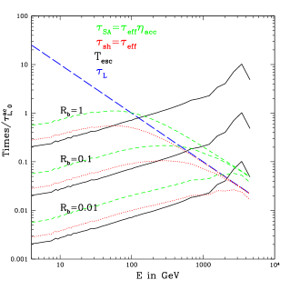
Figure 3: Escape, synchrotron loss and acceleration times in SNRs; black-solid escape, blue-dashed loss, red-dotted assuming pure shock acceleration ($\tau_{\rm ac,sh}=\tau_{\rm eff}$) and green-short dashed assuming pure SA ($\tau_{\rm ac,SA}=\tau_{\rm eff}\eta_{\rm acc})$. All times plotted for three values of ${\cal R}_{a}$, defined in Eq. (45), are in units of synchrotron energy loss time at 100 GeV in the acceleration region of the SNR; $\tau_{{\rm L},0}^{\rm acc}\sim 0.5\times 10^{6}$ yr. Left: Based on Method A. Right: Based on Method B.

These are very similar to the expressions from Method A but are more directly related to the observations and now the energy loss time in the galaxy comes into play.

Thus, in either method we can combine several poorly understood parameters into essentially one unknown; namely the constant coefficient ${\cal R}_{a}$ or ${\cal R}_{b}$. The latter fixes the normalization of the ratio of the effective to accelerated spectra and determines the relative importance of the two terms that appear in the expressions for $\tau_{\rm ac,eff}$ in Eq. (III.4).

IV.4 Results

As mentioned above there is uncertainty associated with values of the spectral indicies and energy cutoffs. In what follows we will set $\alpha_{1}=2,\alpha_{2}=0.6,s=2,E_{\rm CRe}=2$ TeV and $E_{\rm snr}=6$ TeV but will comment on the effects of the uncertainties after presenting the results. Thus, the remaining unknown is the dimensionless factors ${\cal R}_{a}$ and ${\cal R}_{b}$. Before proceeding further we need to estimate their values. Considering the relations between the injection rate deduced from the observations and the observed CRe spectrum, it is clear that $N_{0}^{\rm CRe}\sim\tau_{\rm L,0}^{\rm acc}{\dot{Q}}_{\rm inj,0}^{\rm tr}$ and that ${\cal R}_{a}$ and ${\cal R}_{b}$ should have similar values. Below we estimate their values based on Method B which is more closely related to the observations.

There are reliable estimates for the values of the magnetic fields entering in the expression for ${\cal R}_{b}$ in Eq. (52); as stated above $B_{\rm snr}\sim 15\ \mu$G and using the starlight and infrared photon densities and magnetic field values in the galaxy one gets $B_{\rm eff}\sim 7\ \mu$G e.g., Stawarz et al. (2010). Also using the observed CRe flux (see Fig. 2) of $E^{3}J^{\rm CRe}_{e}(E)|_{E=100\ {\rm GeV}}=120$ GeV²/(s sr m²), we get $N_{0}^{\rm CRe}=5\times\ 10^{-18}\ {\rm cm}^{-3}\ V_{\rm CRe}\sim 3\times 10^{50}$, assuming the poorly known volume of the galaxy that is filled with CRes to be $V_{\rm CRe}\sim 6\times 10^{67}$ cm³. Even less well known are the values of the terms in the square brackets in the numerator of Eq. (52). The rate of occurrence of supernovae is believed to be about several per century but what fraction of these produce active (i.e. CR producing) remnants is not well known. Observations seem to indicate a smaller rate ${\dot{n}}_{\rm snr}$. The active age of SNRs is estimated to be around $10^{4}$ to $10^{5}$ yr, which gives a rough estimate of $V_{\rm snr}{\dot{n}}_{\rm snr}\tau_{\rm snr}\sim 100$. The final factor namely $N_{0}^{\rm snr}$ can be estimated from the observed synchrotron and X-ray radiation intensities of individual SNRs. For example, SNR RXJ1713.7–3946 has an observed peak flux (at X-rays) of $\nu F_{\nu}\sim 600$ eV/(s cm^-2) and a low energy spectrum $F_{\nu}\propto\nu^{-0.5}$. Assuming a distance of 6 kpc, we get a good estimate for the total energy of the synchrotron radiation ${\dot{\cal E}}_{\rm syn}\sim 4\times 10^{36}$ ergs/s. This is related to the accelerated particle spectra as

$${\dot{\cal E}}_{\rm syn}=\int_{0}^{\infty}N^{\rm snr}_{\rm acc}(E){\dot{E}}_{\rm syn}(E)dE,$$ (53)

where ${\dot{E}}_{\rm syn}=E^{2}/(\tau^{\rm acc}_{\rm L,0}E_{0})$ is the synchrotron energy loss rate. For the assumed spectral parameters this gives ${\dot{\cal E}}_{\rm syn}=N_{0}^{\rm snr}E_{\rm snr}/\tau^{\rm acc}_{\rm L,0}$ or $N_{0}^{\rm snr}=6\times 10^{48}$.

Putting all these together we get ${\cal R}_{b}\sim 1$. However this is most likely an overestimation because we have used the observations from a bright SNR. The number of accelerated electrons for an average SNR (including possibly a substantial population of weak and undetected ones) would lower this value considerably. For example, using the general belief that supernovae inject $10^{51}$ ergs into the ISM and that say 10 percent of this going to CRs, with an electron share of one to two percent, we get a number of accelerated electrons smaller by a factor of 10, or $N_{0}^{\rm snr}\sim 10^{48}$ or ${\cal R}_{b}\sim 0.1$. Considering the large uncertainties about all the above numbers, in what follows we present results for three values of ${\cal R}_{a}={\cal R}_{b}=1.0,0.1$ and 0.01 spanning a wide enough range to account for all uncertainties.

Figure 3 shows variation with energy of all time scales obtained by Method A (left) and Method B (right) normalized to the value of synchrotron energy loss time at 100 GeV in the SNR ($\tau_{\rm L,0}^{\rm ac}\sim 0.5\times 10^{6}$ yr). As evident the two methods give very similar results but Method B results end where the observations of CRe spectra become unreliable.

V Interpretation and Discussions

Let us first consider the escape time which is essentially the ratio of the accelerated spectrum to observed CRe spectrum multiplied by the loss time. At energies below $E_{\rm CR}=2$ TeV it is nearly a power law with index $\sim(s-\alpha_{1})=0.7$ in Method A and is $\sim(d\ln j/d\ln E+d\ln h/d\ln E)-(1+\alpha_{1})\sim 0.3$ in Method B, with difference primarily due to the KN effect. $T_{\rm esc}$ starts to increase steeply at $E>$ 1–2 TeV. This rise makes the escape of high energy electrons from the SNRs more difficult, and is the causes of the steep (exponential) decline in the observed CRe spectrum.

The acceleration times for pure shock or pure SA have similar energy dependences (with a factor of $\eta_{\rm acc}\sim 2$ difference between them; with SA requiring a longer time or a lower rate). At low energies these times are dominated by the second term in Eqs. (44) and (51), which makes them proportional to the escape time. Had this trend continued to higher energies the acceleration time would have exceeded the energy loss time which would have caused a spectral cutoff when these times would have been equal (e.g., at 0.1, 0.5, and 3 TeV for ${\cal R}_{b}$ = 1.0, 0.1, and 0.01, respectively; and at smaller values by a factor of about 2 for Method A). Since the deduced SNR electron spectra are observed to cut off at higher energies (6 TeV for RXJ 1713.7), the acceleration time must decrease to remain below the energy loss time as seen in both figures.

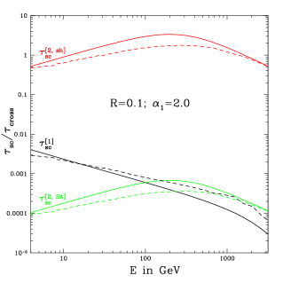
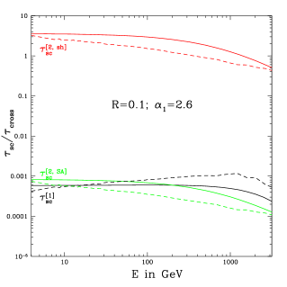
Figure 4: Scattering times obtained from the relation between escape and scattering times in Eq. 11 (black), and the relation between the acceleration and scattering times; Eq. 7 for pure shock acceleration (red) and pure SA from the simple relationship $\tau_{\rm sc}\,^{[2,{\rm SA}]}=\tau_{\rm acc,SA}\beta_{A}^{-2}$ (green), valid for relativistic energies and Alfvénic turbulence ($c\beta_{A}$ is the Alfvén velocity). Solid and dashed curves obtained using Methods A and B, respectively using ${\cal R}=0.1$ for both. Left: For spectral index $\alpha_{1}=2.0$. Right: For spectral index $\alpha_{1}=2.6$.

As evident from the discussion in §II and III we can also obtain the scattering time in the acceleration site. For this purpose we need some information about the background plasma in the acceleration site. The first is the size $L$ of the region. We will use the fiducial value of 10 pc (to include the effects of the chaotic structure of the large scale magnetic field; see Footnote 1) which gives us a crossing time $\tau_{\rm cross}\,\sim 30$ yr. We also need the shock, Alfvén and sound velocities. We shall assume a shock velocity of $10^{4}$ km/s or $\beta_{\rm sh}^{2}\sim 10^{-3}$, and Alfvén velocity of 100 km/s (for $B\sim 15$ $\mu$G, $n=0.1$ cm^-3) or $\beta_{A}^{2}\sim 10^{-7}$, so that the Alfvén Mach numbers is very large as one needs for efficient shock acceleration. For such such high Mach numbers the compression ratio $r=4$ and $\zeta=1/4$.

There are, however, two different ways of obtaining the scattering time. The first way, which is common for both shock or SA, comes from the relation between the escape and scattering times, which if we assume a random walk process of escape is described by Eq. (11) and involves the crossing time. Given that $T_{\rm esc}>10^{3}\ {\rm yr}\gg\tau_{\rm cross}\,\sim$ 30 yr we obtain the first estimate for the scattering time as:

$$\tau_{\rm sc}\,^{[1]}=\frac{\tau^{2}_{\rm cross}}{T_{\rm esc}}\sim 0.025\ {\rm yr}~{}\left(\frac{L}{10\ {\rm pc}}\right)^{2}\left(\frac{4\times 10^{4}\ {\rm yr}}{T_{\rm esc}}\right),$$ (54)

which as expected is much shorter than the crossing time. Here and in what follows the numerical values are calculated for $E=100$ GeV and ${\cal R}=0.1$.

The second method of determining $\tau_{\rm sc}\,$ comes from the relation between the acceleration and scattering times. For pure shock acceleration $\tau_{\rm ac,sh}=\tau_{\rm ac,eff}$ and as seen in Eqs. (7) and (9) the energy dependence of the scattering and acceleration times should be similar but their relative value depends on the shock velocity, the factor $\zeta$, and for perpendicular shocks on $\eta=\kappa_{\|}/\kappa_{\perp}$. Neglecting the latter for now we get

$$\tau_{\rm sc}\,^{[2,{\rm sh}]}=\zeta\left(\frac{u_{\rm sh}}{c}\right)^{2}\tau_{\rm ac,sh}\sim 10\ {\rm yr}\left(\frac{\beta^{2}_{\rm sh}}{10^{-3}}\right)\left(\frac{\tau_{\rm ac,sh}}{4\times 10^{4}\ {\rm yr}}\right),$$ (55)

which is about the crossing time and much larger than the the first estimate of scattering time. It also has a different energy dependence. As can be seen in Figure 4 (left), for the spectral indexes ($\alpha_{1}=2,s=2.6$) assumed above the first estimate (black curves) decreases monotonically with energy while the second (red curves) first increases with energy and then declines at higher energies. The difference in energy dependence at low energies comes from the fact that here $T_{\rm esc}\propto\tau_{\rm ac,eff}$ [see Eqs. (46) and (47)] making $\tau_{\rm sc}\,^{[2,{\rm sh}]}\propto 1/\tau_{\rm sc}\,^{[1,{\rm sh}]}(\propto E^{\alpha_{1}-s}$, for Method A). This difference will be less severe for a steeper SNR electron spectra (i.e. for $\alpha_{1}$ closer to $s$), which is the case in some SNRs. For example, in SNR S1993J with radio spectral index of $\sim 0.8$ one gets $\alpha_{1}\sim 2.6$ (Weiler et al. (2010)). As shown in Figure 4 (right) using $\alpha_{1}=2.6$ we get similar energy dependence for both estimates (and both methods).

However, as shown above the absolute values of the scattering time deduced from the two curves are different by a large factor:

$$\frac{\tau_{\rm sc}\,^{[2,{\rm sh}]}}{\tau_{\rm sc}\,^{[1]}}=4000\left(\frac{\beta^{2}_{\rm sh}}{10^{-3}}\right)\left(\frac{10\ {\rm pc}}{L}\right)^{2}\left({\tau_{\rm sh}T_{\rm esc}\over 1.6\times 10^{9}\ {\rm yr}^{2}}\right).$$ (56)

Agreement can be obtained for a lower shock velocity ($\sim 150$ km/s) and/or a larger crossing time ($L\sim 60$ pc). There is more uncertainty in the first of the above two ways of computing the scattering time; for example, as mentioned above and in Footnote 2, in a chaotic magnetic field of scale $\lambda_{B}\ll L$ the effective crossing time will be larger by $L/\lambda_{B}$, which will reduce the above discrepancy by the square of this factor. Thus, for concordance we require $L^{2}/\lambda_{B}\sim 600$ pc; (e.g., $\lambda_{B}\sim 0.01$ pc for $L=2.5$ pc). As mentioned in connection with Eq. (10), for a perpendicular shock this ratio decreases by the factor $\eta/2$ expected to be much larger than one so that the required conditions may not be as extreme.

More generally, the validity of the use of the random walk relation between escape and scattering times may also be questionable, so that these results may be telling us that the relation of the escape time to the scattering and crossing times is more complicated than given by the random walk hypothesis. For example, in a near perpendicular shock, where particles spiral up and down the surface of the shock and escape when they are scattered perpendicular to the shock front, the escape time may be proportional to the diffusion coefficient perpendicular to the magnetic field giving $\tau_{\rm sc}\,^{[1]}\propto T_{\rm esc}/\eta$, which could bring the shape and value of the first estimate closer to that of the second estimate. To our knowledge there has not been much discussion of this aspect of the problem in the literature so that these possibilities require further explorations, which are beyond the scope of this paper.

Stochastic acceleration by turbulence may be important or even dominant if there is weak or no turbulence in the upstream region, conjectured to be generated by the accelerated particles. In this case most of the acceleration may happen in the downstream turbulent region with particle escaping into the ISM once they cross the shock into the upstream region. However, this mechanism also faces similar difficulties. Here the energy dependence of the acceleration time $\tau_{\rm ac,SA}\sim 2\tau_{\rm ac,eff}$ (or energy diffusion time) is related to the scattering time via the relation between $D_{pp}/p^{2}$ and $D_{\mu\mu}$. In most wave-particle interaction scenarios these two coefficients have fairly similar energy dependences especially at relativistic energies. Electrons with energies above few GeV interact mainly with Alfvén or fast mode waves in which case $D_{pp}/p^{2}=D_{\mu\mu}\beta_{A}^{2}\propto E^{q-2}$ so that $\tau_{\rm ac,SA}\propto p^{2}/D_{pp}$ and $\tau_{\rm sc,SA}\propto 1/D_{\mu\mu}$ (see e.g. Pryadko and Petrosian (1997)). Thus, we have a second estimate for scattering time for SA as well:

$$\tau_{\rm sc}\,^{[2,{\rm SA}]}=\tau_{\rm ac,SA}\beta_{A}^{2}=10^{-2}\ {\rm yr}\left(\frac{\beta^{2}_{A}}{10^{-7}}\right)\left(\frac{\tau_{\rm acc,eff}}{10^{5}\ {\rm yr}}\right).$$ (57)

As shown by the green lines in Figure 4, in this case also the energy dependences of $\tau_{\rm sc}\,^{[1]}$ and $\tau_{\rm sc}\,^{[2,{\rm SA}]}$ disagree at low energies for $\alpha_{1}=2$ (left) but they roughly agree at high energies, and, again, the agreement is improved for $\alpha_{1}=2.6$ (right), where both times have almost a flat energy dependence requiring a turbulence spectral index of $q=2$, which is somewhat greater than the Kolmogorov index. Moreover, now the relative absolute values are in better agreement for the assumed values of Alfvén velocity of 100 km/s and effective size of $L\sim 10$ pc.

VI Summary

We consider acceleration of particles in the framework of the leaky box version of the Fokker-Planck kinetic equation, which provides an adequate description of the pitch angle averaged and spatially integrated (over the acceleration region) energy spectrum of the accelerated particles. This equation describes SA by turbulence and/or acceleration by a shock, where the leaky box encloses the upstream and downstream turbulent regions of the shock. Turbulence plays a central role in both mechanisms, with the momentum diffusion coefficient $D_{pp}$ determining the rate of energy diffusion and acceleration in the SA model, and with the pitch angle diffusion coefficient $D_{\mu\mu}$ determining the spatial diffusion coefficient $\kappa\sim v^{2}/D_{\mu\mu}$, hence the rate of acceleration by the shock. In addition, the energy loss rate, shock compression ratio (or Mach number) and relative values of the spatial diffusion coefficients parallel and perpendicular to the magnetic field, and in the upstream and downstream regions, also come into play. In the leaky box scenario the coefficients $D_{pp}$ and $D_{\mu\mu}$ are represented by the energy diffusion coefficient $D_{\rm EE}$ and the escape time $T_{\rm esc}$ of the particles from the acceleration site. Thus, if we can measure the latter two coefficients we can determine the fundamental wave-particle interaction rates and shed light on the nature of turbulence

$\bullet$ As demonstrated in Petrosian and Chen (2010), we can obtain the escape time from the measured spectrum of the accelerated particle $N(E)$ and that of the escaping particles $N(E)/T_{\rm esc}(E)$. We further demonstrate (see Chen and Petrosian (2013)) that with the inversion of the differential kinetic equation into its integral form, we can obtain the energy diffusion coefficient non-parametrically and directly from observations of the two spectra and the energy loss rate of the particles in the acceleration region.

$\bullet$ We also show that the relations between the two unknowns and observables simplifies considerably if the escaping particles lose all their energy in the transport region outside the acceleration site.

$\bullet$ We demonstrate how this procedure can give us the two unknown characteristics of the acceleration mechanism in SNRs using the spectrum of the accelerated electrons deduced from radio, X-ray and gamma-ray observations of the SNRs and the observed galactic CRe spectrum.

$\bullet$ Expressing all the coefficients or rates in terms of their associated timescales (e.g., acceleration and scattering times), we show that the unknown time scales can be expressed in units of the relatively well known synchrotron energy loss time in the SNR and a single parameter which is a combination of various observable scaling factors, such as rate of formation and length of active period of SNRs and other secondary factors.

$\bullet$ We employ two different methods of treatment of the observations and show the deduced energy dependence of escape and acceleration times for some reasonable value of the parameters, which in principle can be known given sufficient detailed observations. In Method A we use the spectrum of injected electrons into the ISM deduced from the observed CRe spectrum (e.g., using GALPROP or other similar models for transport of electrons in the ISM). In Method B we use the observed CRe spectrum directly using a simplified transport dominated and IC losses by starlight which is affected by the KN effects as described in Stawarz et al. (2010).

$\bullet$ For interpretation of the results, we show that we can obtain scattering time ($\tau_{\rm sc}\,\sim 1/D_{\mu\mu}$) of particles in the acceleration region using two different relations between it and the above timescales. The first is from its relation to the escape time, which is mediated by the crossing time ($\tau_{\rm cross}\,=L/c$) as $\tau_{\rm sc}\,=\tau_{\rm cross}^{2}/T_{\rm esc}$ assuming a random walk situation when $T_{\rm esc}\gg\tau_{\rm sc}\,$. The second is from its relation to the acceleration times. For shock acceleration scattering and acceleration times are proportional to each other with proportionality constant being $(u_{\rm sh}/v)^{2}$ (plus factors $\zeta$ and $\eta$). For pure SA of greater than few GeV electrons by Alfvén or fast mode waves there is a similar relation but with proportionality constant of $(v_{A}/v)^{2}$.

$\bullet$We find that, for the values of the parameters used in our calculation (specifically the spectral index $\alpha_{1}=2.0$), the two estimates of the scattering time give very different energy dependences for the scattering time. This discrepancy largely disappears for $\alpha_{1}=2.6$. Given the caveats stressed in our discussion this is not an unlikely resolution of the problem.

$\bullet$ Assuming presence of a sufficient intensity of turbulence both in the upstream and downstream regions of the shock, we expect the acceleration in SNRs to be dominated by the shock, because of the prevailing high Mach numbers. However, for this scenario we find that the absolute values obtained by the two relations are different by a factor of about 1000 for our fiducial values of $10^{4}$ km/s for shock velocity and $L=10$ pc for size. This discrepancy will be smaller for a perpendicular shock. This lead us to our first conclusion that, in addition to a steeper spectrum for accelerated electrons, either these values are off by an order of magnitude, or that the escape time is not related to the crossing time in the simple way one obtains from the random walk scenario. The latter is an important result and needs further exploration.

$\bullet$ On the other hand, in absence of a sufficient intensity of turbulence in the upstream region, whose presence is only conjectured and not established definitely yet, one can have a pure SA of particles in the turbulent downstream region. It turns out that in this scenario the absolute values of the two scattering times roughly agree. This, lead us to the second conclusion that in the SA scenario having a steeper accelerated electron spectrum is sufficient and it requires a spectrum of turbulence that is slightly steeper than Kolmogorov.

These are clearly preliminary results, but they demonstrate the power of the inversion method developed here. A more detailed analysis of the existing data on emission from SNRs and transport of the CRes can provide better values and forms for the observables required for the inversion, and a more detailed analysis of the inversion, e.g., including time dependence, can constrain the models further. These will be addressed in future publications. But we can conclude that the above results indicate that either the spectrum of injected electrons in the ISM deduced from CRe and galactic diffuse emissions (Eq. 30) is incorrect and/or the simple relation between escape and scattering times used assuming the random walk scenario is incorrect. The latter is more likely to be the case and is similar to the conclusion we reached applying these techniques to solar flares. There mirroring of electrons in a converging magnetic field configuration was invoked to resolve a similar discrepancy. Perhaps a complex large scale field geometry can help in SNRs as well. On the other hand, more consistent results are obtained for a pure stochastic acceleration scenario.

References

- Petrosian and Chen (2010) V. Petrosian and Q. Chen, Astrophys. J. 712, L131 (2010), eprint 1002.2673.
- Chen and Petrosian (2013) Q. Chen and V. Petrosian, Astrophys. J. 777, 33 (2013), eprint 1307.1837.
- Fermi (1949) E. Fermi, Phys. Rev. 75, 1169 (1949).
- Petrosian (2012) V. Petrosian, Space Sci. Rev. 173, 535 (2012), eprint 1205.2136.
- Sturrock (1966) P. A. Sturrock, Phys. Rev. 141, 186 (1966).
- Schlickeiser (1989) R. Schlickeiser, Astrophys. J. 336, 243 (1989).
- Pryadko and Petrosian (1997) J. M. Pryadko and V. Petrosian, Astrophys. J. 482, 774 (1997), eprint arXiv:astro-ph/9610148.
- Dung and Petrosian (1994) R. Dung and V. Petrosian, Astrophys. J. 421, 550 (1994).
- Petrosian and Liu (2004) V. Petrosian and S. Liu, Astrophys. J. 610, 550 (2004), eprint arXiv:astro-ph/0401585.
- Chandrasekhar (1943) S. Chandrasekhar, Rev. Modern Phys. 15, 1 (1943).
- Tsytovich (1977) V. N. Tsytovich, Theory of Turbulent Plasma (New York: Pergamon, 1977).
- Hamilton and Petrosian (1992) R. J. Hamilton and V. Petrosian, Astrophys. J. 398, 350 (1992).
- Fermi (1954) E. Fermi, Astrophys. J. 119, 1 (1954).
- Krymsky et al. (1979) G. F. Krymsky, A. I. Kuzmin, S. I. Petukhov, and A. A. Turpanov, in International Cosmic Ray Conference (1979), vol. 2 of International Cosmic Ray Conference, p. 39.
- Lagage and Cesarsky (1983) P. O. Lagage and C. J. Cesarsky, Astron. Astrophys. 125, 249 (1983).
- Drury (1983) L. O. Drury, Rep. Prog. Phys. 46, 973 (1983).
- Dröge and Schlickeiser (1986) W. Dröge and R. Schlickeiser, Astrophys. J. 305, 909 (1986).
- Jokipii (1987) J. R. Jokipii, Astrophys. J. 313, 842 (1987).
- Melrose (2009) D. B. Melrose, in Encyclopedia of Complexity and Systems Science, Part 1, ed. R. A. Meyers (Berlin: Springer), 21 (arXiv:0902.1803) (2009), eprint 0902.1803.
- Steinacker et al. (1988) J. Steinacker, R. Schlickeiser, and W. Dröge, Solar Phys. 115, 313 (1988).
- McTiernan and Petrosian (1990) J. M. McTiernan and V. Petrosian, Astrophys. J. 359, 524 (1990).
- Petrosian and East (2008) V. Petrosian and W. E. East, Astrophys. J. 682, 175 (2008), eprint 0802.0900.
- Stawarz et al. (2010) Ł. Stawarz, V. Petrosian, and R. D. Blandford, Astrophys. J. 710, 236 (2010), eprint 0908.1094.
- Li et al. (2011) H. Li, S. Liu, and Y. Chen, Astrophys. J. 742, L10 (2011), eprint 1110.2857.
- Giordano et al. (2012) F. Giordano, M. Naumann-Godo, J. Ballet, K. Bechtol, S. Funk, J. Lande, M. N. Mazziotta, S. Rainò, T. Tanaka, O. Tibolla, et al., Astrophys. J. 744, L2 (2012), eprint 1108.0265.
- Tanaka et al. (2011) T. Tanaka, A. Allafort, J. Ballet, S. Funk, F. Giordano, J. Hewitt, M. Lemoine-Goumard, H. Tajima, O. Tibolla, and Y. Uchiyama, Astrophys. J. 740, L51 (2011), eprint 1109.4658.
- Brown et al. (1983) J. C. Brown, I. J. D. Craig, and D. B. Melrose, Astrophys. Space Sci. 92, 105 (1983).
- Johns and Lin (1992) C. M. Johns and R. P. Lin, Solar Phys. 137, 121 (1992).
- Lazendic et al. (2004) J. S. Lazendic, P. O. Slane, B. M. Gaensler, S. P. Reynolds, P. P. Plucinsky, and J. P. Hughes, Astrophys. J. 602, 271 (2004), eprint arXiv:astro-ph/0310696.
- Weiler et al. (2010) K. W. Weiler, N. Panagia, R. A. Sramek, S. D. Van Dyk, C. J. Stockdale, and C. L. Williams, Mem. Societa Astronomica Italiana 81, 374 (2010).
- Krymskii (1977) G. F. Krymskii, Akademiia Nauk SSSR Doklady 234, 1306 (1977).
- Axford et al. (1978) W. I. Axford, E. Leer, and G. Skadron, in Cosmophysics, edited by V. A. Dergachev and G. E. Kocharov (1978), pp. 125–134.
- Bell (1978) A. R. Bell, Monthly Notices of the RAS 182, 147 (1978).
- Blandford and Ostriker (1978) R. D. Blandford and J. P. Ostriker, Astrophys. J. 221, L29 (1978).
- Prantzos et al. (1986) N. Prantzos, C. Doom, C. De Loore, and M. Arnould, Astrophys. J. 304, 695 (1986).
- Woosley et al. (2002) S. E. Woosley, A. Heger, and T. A. Weaver, Reviews of Modern Physics 74, 1015 (2002).
- Adriani et al. (2011) O. Adriani, G. C. Barbarino, G. A. Bazilevskaya, R. Bellotti, M. Boezio, E. A. Bogomolov, M. Bongi, V. Bonvicini, S. Borisov, S. Bottai, et al., Phys. Rev. Lett. 106, 201101 (2011), eprint 1103.2880.
- Aharonian et al. (2008) F. Aharonian, A. G. Akhperjanian, U. Barres de Almeida, A. R. Bazer-Bachi, Y. Becherini, B. Behera, W. Benbow, K. Bernlöhr, C. Boisson, A. Bochow, et al., Phys. Rev. Lett. 101, 261104 (2008), eprint 0811.3894.
- Ackermann et al. (2010) M. Ackermann, M. Ajello, W. B. Atwood, L. Baldini, J. Ballet, G. Barbiellini, D. Bastieri, B. M. Baughman, K. Bechtol, F. Bellardi, et al., Phys. Rev. D 82, 092004 (2010), eprint 1008.3999.
- Moskalenko and Strong (1998) I. V. Moskalenko and A. W. Strong, Astrophys. J. 493, 694 (1998), eprint arXiv:astro-ph/9710124.
- Strong et al. (2011) A. W. Strong, E. Orlando, and T. R. Jaffe, Astron. Astrophys. 534, A54 (2011), eprint 1108.4822.
- Di Bernardo et al. (2013) G. Di Bernardo, C. Evoli, D. Gaggero, D. Grasso, and L. Maccione, J. Cosmo. Astropart. Phys. 3, 036 (2013), eprint 1210.4546.
- Schlickeiser and Ruppel (2010) R. Schlickeiser and J. Ruppel, New J. Phys. 12, 033044 (2010), eprint 0908.2183.