Gains from switching and evolutionary stability in multi-player matrix games

Abstract

In this paper we unify, simplify, and extend previous work on the evolutionary dynamics of symmetric $N$-player matrix games with two pure strategies. In such games, gains from switching strategies depend, in general, on how many other individuals in the group play a given strategy. As a consequence, the gain function determining the gradient of selection can be a polynomial of degree $N-1$. In order to deal with the intricacy of the resulting evolutionary dynamics, we make use of the theory of polynomials in Bernstein form. This theory implies a tight link between the sign pattern of the gains from switching on the one hand and the number and stability properties of the rest points of the replicator dynamics on the other hand. While this relationship is a general one, it is most informative if gains from switching have at most two sign changes, as it is the case for most multi-player matrix games considered in the literature. We demonstrate that previous results for public goods games are easily recovered and extended using this observation. Further examples illustrate how focusing on the sign pattern of the gains from switching obviates the need for a more involved analysis.

Keywords. evolutionary game theory, multi-player matrix games, replicator dynamics, public goods games, gains from switching, polynomials in Bernstein form

• Faculty of Business and Economics
  University of Basel
  Peter Merian-Weg 6, CH-4002 Basel, Switzerland
  Current address:
  Research Group for Evolutionary Theory
  Max Planck Institute for Evolutionary Biology
  August-Thienemann-Str. 2, 24306 Plön, Germany
  e-mail: pena@evolbio.mpg.de
  

• Department of Ecology and Evolution
  University of Lausanne
  Le Biophore, CH-1015 Lausanne, Switzerland
  e-mail: laurent.lehmann@unil.ch
  

• Faculty of Business and Economics
  University of Basel
  Peter Merian-Weg 6, CH-4002 Basel, Switzerland
  e-mail: georg.noeldeke@unibas.ch
  

• Corresponding author.

1 Introduction

Game theory has been widely applied to evolutionary biology (Maynard Smith, 1982; Eshel, 1996; Rousset, 2004; Vincent and Brown, 2005; Broom and Rychtář, 2013). Evolutionary game theory has been instrumental in explaining the evolution of traits as diverse as the sex ratio, dispersal, mate competition, parasite transmission, flowering time, cooperation, policing, dormancy, and anisogamy (e.g., Comins et al., 1980; Maynard Smith, 1982; Clark and Mangel, 1986; Frank, 1987; Bulmer, 1994; Frank, 1995; Bulmer and Parker, 2002; Foster, 2004; Rousset, 2004; Otto and Day, 2007).

Evolutionary models of these traits often assume “playing the field” type of interactions (Maynard Smith, 1982, p. 23), where the payoff to an individual depends on an average property of the population or the group with which it interacts. There are also many situations, however, where the payoff to an individual depends critically on the strategy profile in the population (or its group) and where the actions of different individuals cannot be averaged; that is, mass action does not apply. Typical examples involve collective action problems in moderately sized groups, where the change in behavior by a single individual can result in a large, discontinuous change in payoffs to others (e.g., Boyd and Richerson, 1988). Such collective action problems have been modeled as multi-player (or multi-person) matrix games (Broom et al., 1997; Kurokawa and Ihara, 2009; Gokhale and Traulsen, 2010). Except for the very special cases in which group size is taken to be equal to two (so that the well-developed theory of two-player matrix games can be applied, cf. Weibull, 1995; Hofbauer and Sigmund, 1998; Cressman, 2003) or the payoff structure is linear (as in the standard model of the $N$-person prisoner’s dilemma) such games have proven difficult to analyze.

The intrinsic complexity of multi-player matrix games is already evident for the case of symmetric games with two pure strategies A and B on which we focus in this paper. For these games, the average payoff difference in a large and well-mixed population is given by the so-called gain function (Bach et al., 2006)

$$g(x)=\sum_{k=0}^{n}\binom{n}{k}x^{k}(1-x)^{n-k}d_{k}.$$

Here $n$ is the number of co-players of a focal player (so that $N=n+1$ is the group size), $x$ is the population fraction of A-strategists, and $d_{k}$ is the gain a focal player would obtain if switching from strategy B to strategy A when $k$ other group-members play A. The evolutionary solution of the game (such as the set of evolutionarily stable strategies, ESSs, or the set of stable rest points of the replicator dynamics) involves not only finding the roots of the gain function $g(x)$ (a polynomial of degree $n$) but also determining the behavior of $g(x)$ in the vicinity of such roots. While this is straightforward for two-player games and multi-player games with a linear payoff structure (for which $g(x)$ linear in $x$), it is less evident for more general multi-player games. Indeed, non-linear payoff structures in groups of size larger than five may lead to polynomials of degree greater than four that, in general, cannot be solved analytically (Clark, 1984).

In order to deal with such complexity, the vast majority of previous works on multi-player matrix games has considered particular functional forms for the specification of the payoffs and has resorted to lengthy algebra or numerical methods to study the models (Joshi, 1987; Boyd and Richerson, 1988; Dugatkin, 1990; Weesie and Franzen, 1998; Hauert et al., 2006; Zheng et al., 2007; Cuesta et al., 2008; Pacheco et al., 2009; Archetti, 2009; Souza et al., 2009; Archetti and Scheuring, 2011; van Segbroeck et al., 2012). This way some non-linear public goods games, including multi-player extensions of well-known two-person matrix games such as the stag hunt (Skyrms, 2004) and the snowdrift game (Sugden, 1986), have been characterized on a case-by-case basis.

In contrast to these efforts, Motro (1991) and Bach et al. (2006) have taken a more systematic approach to the study of non-linear public goods games. Both of these papers consider situations in which each contributor to a public good pays a constant cost, whereas the benefit from the public good, which is obtained by all players, is a function of the number of contributors. Motro (1991) proves that in this case the replicator dynamics has at most one interior rest point if the benefit is concave or convex in the number of contributors. He also provides necessary and sufficient conditions for the existence of such a rest point and characterizes the stability property of all rest points. In a similar spirit, Bach et al. (2006) find sufficient conditions on the shape of the benefits such that there exists a critical cost level with the property that for costs below such level the replicator dynamics has two interior rest points, whereas for higher costs there is no interior rest point.

More recently, Gokhale and Traulsen (2010) have discussed the relationship between the sign pattern of the gains from switching and the number of interior rest points of the replicator dynamics. Specifically, these authors observe that the replicator dynamics has a single interior rest point if the sequence $(d_{0},d_{1},\ldots,d_{n})$, which we refer to as the gain sequence, has exactly one sign change. Gokhale and Traulsen (2010) also note that the direction of selection (as given by the sign of the gain function $g(x)$) cannot have more sign changes than the gain sequence. This implies that the number of sign changes of the gain sequence provides an upper bound on the number of interior rest points of the replicator dynamics. The latter observation is also made in Hauert et al. (2006) and Cuesta et al. (2007).

In this paper, we show how sign-change conditions like the ones discussed in Gokhale and Traulsen (2010) can be refined by using the fact that the gain function $g(x)$ is a particular kind of polynomial, known as polynomial in Bernstein form (or Bernstein polynomial) with coefficients given by the gain sequence $(d_{0},d_{1},\ldots,d_{n})$. Polynomials in Bernstein form are rich in shape-preserving properties, long recognized in the fields of approximation theory (Bernstein, 1912; Lorentz, 1986; DeVore and Lorentz, 1993) and computer aided geometric design (Yamaguchi and Yamaguchi, 1988; Farin and Hoschek, 2002; Farouki, 2012). Our analysis rests on the variation-diminishing property of Bernstein polynomials and a property that we refer to as the preservation of initial and final signs. These properties provide a tight link between the sign pattern of the gain sequence and the sign pattern of the gain function. In particular, if the gain sequence has at most two sign changes, a full characterization of the possible dynamic regimes is easily obtained.

For most of the collective action problems that have been modeled as multi-player matrix games it is straightforward to determine the sign pattern of the gain sequence. Moreover, because the gain sequences of these games have at most two sign changes, our characterization results provide all the information necessary to recover the results on the number and stability of rest points obtained in previous studies. We demonstrate these claims for two classes of public goods games, namely threshold games (e.g., Dugatkin, 1990; Weesie and Franzen, 1998; Zheng et al., 2007; Souza et al., 2009), and constant cost games (e.g., Motro, 1991; Bach et al., 2006; Hauert et al., 2006; Pacheco et al., 2009; Archetti and Scheuring, 2011), and two additional examples taken from van Segbroeck et al. (2012) and Hauert et al. (2006), thus supporting the claim that the approach developed here unifies, simplifies, and extends much of the previous work on multi-player matrix games.

2 Model

Interactions occur in groups of size $N=n+1$, in which a focal individual plays a game against $n$ co-players or opponents. Each individual can choose between one of two different pure strategies, A and B. The game is symmetric so that, from the focal’s point of view, any two co-players are exchangeable.

Let $a_{k}$ denote the payoff to an individual choosing A when $k$ opponents choose A (and hence $n-k$ co-players choose B); likewise, let $b_{k}$ denote the payoff to an individual choosing B when $k$ opponents choose A. Also let

$$d_{k}\equiv a_{k}-b_{k}$$

denote the gain the focal player makes from choosing A over B, taking the choices of other players ($k$ playing A and $n-k$ playing B) as given. The parameters $d_{k}$, which describe the gains from switching, are collected in the gain sequence $\mathbf{d}=(d_{0},d_{1},\ldots,d_{n})$. We assume $\mathbf{d}\not=\bm{0}$, thus excluding the trivial and uninteresting case in which payoffs are independent of the actions chosen.

Evolution occurs in an infinitely large and well-mixed population with groups randomly formed by binomial sampling. Hence, if the frequency of A-strategists in the whole population is $x$, the average payoffs obtained by an A-strategist and a B-strategist are respectively given by

$$\pi_{\mathrm{A}}(x)=\sum_{k=0}^{n}\binom{n}{k}x^{k}(1-x)^{n-k}a_{k}$$

and

$$\pi_{\mathrm{B}}(x)=\sum_{k=0}^{n}\binom{n}{k}x^{k}(1-x)^{n-k}b_{k}.$$

We assume that the rules of transmission of the strategies (whether genetically encoded or individually or socially learned) are such that the frequency $x$ of A-strategists in the population can be described by the replicator dynamics (Taylor and Jonker, 1978; Hofbauer and Sigmund, 1998)

$$\frac{\mathrm{d}x}{\mathrm{d}t}=x(1-x)g(x),$$ (1)

where $g(x)=\pi_{\mathrm{A}}(x)-\pi_{\mathrm{B}}(x)$ is the gain function (Bach et al., 2006) given by

$$g(x)=\mathcal{B}_{n}(x;\mathbf{d})\equiv\sum_{k=0}^{n}\binom{n}{k}x^{k}(1-x)^{n-k}d_{k}.$$ (2)

As we have already mentioned in the Introduction, the gain function is a polynomial in Bernstein form (also known as a Bernstein polynomial, cf. Farouki (2012)). This is made explicit by the notation we introduce in (2), where the Bernstein operator $\mathcal{B}_{n}$ maps the vector of Bernstein coefficients $\mathbf{d}\in\mathbb{R}^{n+1}$ into the polynomial $\sum_{k=0}^{n}\binom{n}{k}x^{k}(1-x)^{n-k}d_{k}$ in the variable $x\in[0,1]$.

The replicator dynamics (1) has two trivial rest points at $x=0$ (where the whole population consists of B-strategists) and $x=1$ (where the whole population consists of A-strategists). Interior rest points $0<x^{*}<1$ are given by the solutions of the equation $g(x^{*})=0$. Because $g(x)$ is a polynomial of degree at most $n$ (and we have assumed $\mathbf{d}\not=\bm{0}$) the replicator dynamics can have at most $n$ interior rest points, corresponding to $n$ simple roots of $g(x)$ in the open interval $(0,1)$. In the two-strategy case we analyze here, rest points of the replicator dynamics can be either (locally asymptotic) stable or unstable. Stability of a rest point $x^{*}$ requires that $(x-x^{*})(g(x)-g(x^{*}))<0$ holds for all $x\not=x^{*}$ in a neighborhood of $x^{*}$. Since the stable rest points of the replicator dynamics correspond to ESSs for the multi-player game (Bach et al., 2006), our following results about stable rest points of the replicator dynamics carry over to ESSs without any changes.

Remark 1.

The gain function $g(x)$ given in (2) can also be interpreted as the selection gradient on a continuously varying mixed strategy $x$ (denoting the probability that action A is played), evolving according to the traditional breeder’s equation or the canonical equation of adaptive dynamics (Dieckmann and Law, 1996), so that the dynamics is of the form

$$\frac{\mathrm{d}x}{\mathrm{d}t}=v(x)g(x),$$

for some measure $v(x)$ of genetic variance (Kirkpatrick and Rousset, 2005). Hence, all our subsequent results pertaining to polymorphic equilibria in pure strategies can also be interpreted in terms of monomorphic equilibria for mixed strategies.

3 Sign patterns and (the stability of) rest points

The fact that the gain function is a polynomial in Bernstein form implies a tight link between the sign pattern of the gain sequence on the one hand and the sign pattern and number of roots of the gain function on the other hand. This is due to two properties of Bernstein polynomials, namely the preservation of initial and final signs and the variation diminishing property (see Properties 1 and 2 below). Because roots of the gain function correspond to interior rest points of the replicator dynamics and the sign pattern of the gain function informs us about the direction of selection at the trivial rest points as well as changes in the direction of selection at interior rest points, general results about the number and stability of rest points follow immediately (see Results 1 and 2). These results hold for any non-zero gain sequence, allow for interior rest points at which the direction of selection does not change, and provide more detailed information about the number of rest points and stable equilibria than the observations made by Cuesta et al. (2007) and Gokhale and Traulsen (2010). Results 3 to 5 summarize the implications of the general results for gain sequences with at most two sign changes, providing the basis for our subsequent analysis.

3.1 Preliminaries

To proceed, we require some terminology and notation to describe sign patterns (see Brown et al., 1981) and other relevant shape properties of gain sequences and gain functions. The same notation and terminology applies to other sequences and functions we encounter in our analysis.

Let $I(\mathbf{d})$ denote the sign (either $+$ or $-$) of the first non-zero entry in the sequence $\mathbf{d}$. Likewise, let $F(\mathbf{d})$ denote the sign of the last non-zero entry in $\mathbf{d}$. We refer to $I(\mathbf{d})$ and $F(\mathbf{d})$ as the initial and final signs of the gain sequence $\mathbf{d}$. We also denote by $S(\mathbf{d})$ the number of sign changes between consecutive entries in $\mathbf{d}$ after zero entries have been eliminated. Obviously, $0\leq S(\mathbf{d})\leq n$.

As we have assumed $\mathbf{d}\not=\bm{0}$, there exists a neighborhood of $x^{*}=0$ such that the sign of $g(x)$ is either $+$ or $-$ for all $x\not=0$ in this neighborhood. We define the initial sign $I(g)$ of $g(x)$ as the sign of $g(x)$ in such neighborhood, and define the final sign $F(g)$ in an analogous way. Note that $I(g)$ coincides with the sign of $g(0)$ if $g(0)\not=0$ holds. Similarly, if $g(1)\not=0$ holds, then $F(g)$ coincides with the sign of $g(1)$. The number of sign changes $S(g)$ of the function $g(x)$ in the interval $(0,1)$ is the number of times it crosses the $x$-axis in $(0,1)$.

The notation $\Delta\mathbf{d}=(\Delta d_{0},\ldots,\Delta d_{n-1})$, where $\Delta d_{k}\equiv d_{k+1}-d_{k}$, denotes the (first) forward difference of the sequence $\mathbf{d}$. The second forward difference of the sequence $\mathbf{d}$ is $\Delta^{2}\mathbf{d}=(\Delta^{2}d_{0},\ldots,\Delta^{2}d_{n-2})$, where $\Delta^{2}d_{k}\equiv\Delta d_{k+1}-\Delta d_{k}$. These forward differences can be viewed as the counterparts to the first and second derivatives of a real function and are a useful tool for describing the shape of a sequence. In particular, the sequence $\mathbf{d}$ is increasing (resp. decreasing) if $\Delta\mathbf{d}\geq\bm{0}$ ($\Delta\mathbf{d}\leq\bm{0}$) holds, convex (resp. concave) if $\Delta^{2}\mathbf{d}\geq\bm{0}$ (resp. $\Delta^{2}\mathbf{d}\leq\bm{0}$) holds, and unimodal (resp. anti-unimodal) if the sequence $\Delta\mathbf{d}$ has a single sign change from positive to negative (resp. from negative to positive). Mutatis mutandis the same definitions apply to the gain function $g(x)$. For instance, a gain function is unimodal if its first derivative $g^{\prime}(x)$ has one sign change from positive to negative and is concave if its second derivative satisfies $g^{\prime\prime}(x)\leq 0$ for all $0\leq x\leq 1$.

3.2 Stability of trivial rest points

One important property of the Bernstein operator $\mathcal{B}_{n}$ is that it preserves end-points, i.e. $g(0)=\mathcal{B}_{n}(0;\mathbf{d})=d_{0}$ and $g(1)=\mathcal{B}_{n}(1;\mathbf{d})=d_{n}$ (Farouki, 2012). From this, it is immediate that the initial and final signs of $g(x)$ and $\mathbf{d}$ coincide in the case when $d_{0}\not=0$ and $d_{n}\not=0$. We show in Appendix A that the same conclusion obtains in general, so that we have the following property.

Property 1 (Preservation of initial and final signs).

The initial and final signs of $g(x)$ and $\mathbf{d}$ coincide. That is,

$$I(g)=I(\mathbf{d})\text{ and }F(g)=F(\mathbf{d}).$$

The initial sign of $g(x)$ describes the direction of selection in a vicinity of the trivial rest point $x=0$, so that the rest point $x=0$ is stable if and only if the initial sign of $g(x)$ is negative. Similarly, the rest point $x=1$ is stable if and only if the final sign of $g(x)$ is positive. Hence, Property 1 implies that the initial and final signs of the gain sequence are all the information required to determine the stability of the trivial rest points. This is explicitly stated in the following result.

Result 1 (Stability of trivial rest points).

2. The rest point $x=0$ is stable if and only if $I(\mathbf{d})=-$.

3. The rest point $x=1$ is stable if and only if $F(\mathbf{d})=+$.

The first part of Result 1 asserts that strategy A is disadvantageous when rare if and only if the first non-zero element in the gain sequence is negative. The second part is the assertion that strategy A is advantageous when common if and only if the last non-zero element in the gain sequence is positive.

3.3 Number of (stable) interior rest points

Let $R(g)\geq 0$ denote the number of roots of $g(x)$ in the interval $(0,1)$, counting roots according to their multiplicity. The following is the variation diminishing property of Bernstein polynomials.

Property 2 (Variation diminishing property).

2. The number of roots of $g(x)$ on $(0,1)$ is equal to the number of sign changes of $\mathbf{d}$ or less by an even amount. That is,

   $$R(g)=S(\mathbf{d})-2i,\text{ where }i\geq 0\text{ is an integer}.$$ (3)

3. The number of sign changes of $g(x)$ is equal to the number of sign changes of $\mathbf{d}$ or less by an even amount. That is,

   $$S(g)=S(\mathbf{d})-2j,\text{ where }j\geq i\text{ is an integer}.$$ (4)

The first part of the variation-diminishing property (see e.g. Farouki (2012)) follows from Descartes’ rule of signs, which hence can be said to “carry over” to polynomials in Bernstein form. The second part follows from the first upon observing that $x\in(0,1)$ is the location of a sign change of $g(x)$ if and only if $x$ is a root of $g(x)$ with odd multiplicity, so that $S(g)$ is either equal to $R(g)$ or less by an even amount.

As the interior rest points of the replicator dynamics coincide with the roots of $g(x)$, Property 2.1 applies as stated to the interior rest points of the replicator dynamics. In particular, as noted by Cuesta et al. (2007) and Gokhale and Traulsen (2010), the number of sign changes of the gain sequence $\mathbf{d}$ provides an upper bound on the number of interior rest points. If the number of sign changes of $\mathbf{d}$ is odd, (3) implies that $R(g)$ is odd. Consequently, the replicator dynamics possesses at least one interior rest point in this case.

Stability of an interior rest point is equivalent to the requirement that the sign of $g(x)$ changes from $+$ to $-$ at the rest point. As sign changes must alternate and initial signs are preserved (Property 1), the second part of the variation diminishing property yields the following result.

Result 2 (Number of stable interior rest points).

Let $\ell$ denote the number of stable interior rest points of the replicator dynamics and let $j\geq 0$ be the integer appearing in the statement of Property 2.2.

1. If $S(\mathbf{d})$ is even, then $\ell=S(g)/2=S(\mathbf{d})/2-j$.

2. If $S(\mathbf{d})$ is odd and $I(\mathbf{d})=-$, then $\ell=(S(g)-1)/2=(S(\mathbf{d})-1)/2-j$.

3. If $S(\mathbf{d})$ is odd and $I(\mathbf{d})=+$, then $1\leq\ell=(S(g)+1)/2=(S(\mathbf{d})+1)/2-j$.

3.4 Special cases

It will be convenient to summarize the relationship between the sign patterns of the gain sequence and the rest points of the replicator dynamics for the cases in which the gain sequence has at most two sign changes. We also provide simple sufficient conditions ensuring that a gain sequence has at most one, resp. two sign changes.

3.4.1 Gain sequences with one or no sign change

When the gain sequence has no or one sign change, the variation diminishing property implies that the number of roots and the number of sign changes of the gain function both coincide with the number of sign changes of the gain sequence. In particular, Result 2 holds with $j=0$. Combining these observations with Result 1 then shows that for games with gain sequences having at most one sign change, the sign pattern of the gain sequence contains all the information required to determine the number and stability of rest points. For later reference we state the ensuing case distinction in the following result.

Result 3 (Gain sequences with no or one sign change).

2. If the gain sequence has no sign changes, then the replicator dynamics has no interior rest points. Moreover

   1. If $I(\mathbf{d})=-$, then $x=0$ is stable and $x=1$ is unstable.

   2. If $I(\mathbf{d})=+$, then $x=0$ is unstable and $x=1$ is stable.

3. If the gain sequence has a single sign change, then the replicator dynamics has a unique interior rest point $x^{*}$. Moreover:

   1. If $I(\mathbf{d})=-$, then $x=0$ and $x=1$ are stable, and $x^{*}$ is unstable.

   2. If $I(\mathbf{d})=+$, then $x=0$ and $x=1$ are unstable, and $x^{*}$ is stable.

The four possible dynamical regimes appearing in Result 3 correspond to the cases that are familiar from the evolutionary analysis of symmetric two-player games with two pure strategies (see, e.g. Cressman, 2003, Section 2.2). This is, of course, not a coincidence: such two-player games are nothing but the special case of our model with $n=1$ and thus feature gain sequences with at most one sign change.

A simple sufficient condition for the applicability of Result 3 is that the gain sequence is monotonic, that is, either increasing or decreasing. It is clear that an increasing gain sequence can have at most one sign change and that such a sign change occurs if and only if $d_{0}<0<d_{n}$. In this case, the rest points of the replicator dynamics are characterized by Result 3.2.a. The other two possibilities for an increasing gain sequence, namely $d_{n}\leq 0$ and $d_{0}\geq 0$, are covered by Result 3.1.a and Result 3.1.b, respectively. Similarly, for a decreasing gain sequence only three of the four scenarios described in Result 3 are possible, with a stable interior rest point occurring if and only if $d_{0}>0>d_{n}$.

3.4.2 Gain sequences with two sign changes

If the gain sequence has two sign changes, its initial and final signs coincide. Suppose they are both negative. Then, by the preservation of initial and final signs (Property 1), the same is true for the initial and final signs of $g(x)$. In particular, as indicated by Result 1, the rest point $x=0$ is stable and the rest point $x=1$ is unstable. Further, the first part of the variation diminishing property implies that the replicator dynamics has either (i) two distinct interior rest points (which correspond to simple roots in which $g(x)$ crosses zero), (ii) one interior rest point (corresponding to a double root in which $g(x)$ touches, but does not cross zero), or (iii) no interior rest point. In the first of these cases $g(x)$ has two sign changes and the larger of the two interior rest points is stable. In the other two cases $g(x)$ has no sign change and, consequently, no stable interior rest point. Considering the maximal value of $g(x)$ on $[0,1]$, which we denote by $\bar{g}$, provides a convenient way to describe which of these three cases arises. In particular, for $\bar{g}<0$ there is no interior rest point, for $\bar{g}=0$ there is exactly one interior rest point, and for $\bar{g}>0$ there are two interior rest points. Analogous reasoning can be applied for the case in which the initial and final signs are both positive. These considerations are summarized in the following result.

Result 4 (Gain sequences with two sign changes).

Let $\bar{g}=\max_{0\leq x\leq 1}g(x)$ and $\underline{g}=\min_{0\leq x\leq 1}g(x)$. Then:

1. If $S(\mathbf{d})=2$ and $I(\mathbf{d})=-$ the rest point $x=0$ is stable and the rest point $x=1$ is unstable. Further:

   1. if $\bar{g}<0$, the replicator dynamics has no interior rest points.

   2. if $\bar{g}=0$, then the replicator dynamics has one interior rest point $\hat{x}$ which is unstable.

   3. if $\bar{g}>0$, the replicator dynamics has one unstable rest point $x_{\mathrm{L}}$ and one stable rest point $x_{\mathrm{R}}$, satisfying $0<x_{\mathrm{L}}<x_{\mathrm{R}}<1$.

2. If $S(\mathbf{d})=2$ and $I(\mathbf{d})=+$ the rest point $x=0$ is unstable and the rest point $x=1$ is stable. Further:

   1. If $\underline{g}>0$, the replicator dynamics has no interior rest points.

   2. If $\underline{g}=0$, the replicator dynamics has one interior rest point $\hat{x}$ which is unstable.

   3. If $\underline{g}<0$, the replicator dynamics has one stable rest point $x_{\mathrm{L}}$ and one unstable rest point $x_{\mathrm{R}}$, satisfying $0<x_{\mathrm{L}}<x_{\mathrm{R}}<1$.

It is evident from the case distinctions appearing in Result 4 that for gain sequences with two sign changes, information beyond the one contained in the sign pattern of the gain sequence is required to determine the number of interior rest points. However, the additional information required takes a simple form (namely, the knowledge of the maximal, resp. minimal value of the gain function), which is amenable to further analysis.

Remark 2.

If a gain sequence has more than two sign changes, Results 1 and 2 still provide useful information about the possible range of dynamical scenarios, but determining which of these scenarios arises becomes much harder than in the case of at most two sign changes. To illustrate this, consider the case $S(\mathbf{d})=3$ and suppose $I(\mathbf{d})=+$. We then have $F(\mathbf{d})=-$, implying that both trivial rest points are unstable (Result 1). Furthermore, there are either one or two stable interior rest points (Result 2). In the second of these cases there must exist a single unstable interior rest point, in the first case there is either no unstable interior rest point or one unstable interior rest point which corresponds to a root of the gain function with multiplicity two (Property 2.1).

3.4.3 Unimodal gain sequences

Unimodality or anti-unimodality is a simple sufficient condition ensuring that a gain sequence has at most two sign changes. Furthermore, a complete classification of the possible dynamic scenarios is easily obtained. Here we demonstrate these claims for the unimodal case; the argument (and result) for the anti-unimodal case is analogous.

Our argument relies on the identity

$$g^{\prime}(x)=n\mathcal{B}_{n-1}(x;\Delta\mathbf{d}),$$ (5)

which is a classical result in approximation theory, known as the derivative property of polynomials in Bernstein form (see e.g. Lorentz, 1986; DeVore and Lorentz, 1993; Farouki, 2012). By (5) the derivative $g^{\prime}(x)$ is proportional to a Bernstein polynomial with coefficients $\Delta\mathbf{d}$. We may thus apply Properties 1 and 2 to the relationship between the sign pattern of $\Delta\mathbf{d}$ and the roots and sign pattern of $g^{\prime}(x)$. Recalling that for a unimodal gain sequence $\Delta\mathbf{d}$ has a single sign change from positive to negative, it follows that unimodality of the gain sequence implies unimodality of the gain function. Moreover, applying the first part of the variation diminishing property, there exists a unique $0<\hat{x}<1$ satisfying the first order condition $g^{\prime}(\hat{x})=0$. Unimodality of $g(x)$ implies that $\hat{x}$ is the unique solution to the problem $\max_{0\leq x\leq 1}g(x)$ appearing in the statement of Result 4. In particular, we have $\bar{g}=g(\hat{x})$.

It is clear that a unimodal gain function can have at most one sign change in its increasing part (which then must be from negative to positive) and at most one sign change in its decreasing part (which then must be from positive to negative). Moreover, a sign change in the increasing part occurs if and only if $g(0)<0<g(\hat{x})$ and a sign change in the decreasing part occurs if and only if $g(1)<0<g(\hat{x})$. Combining these observations yields the following result, refining Results 3 and 4 for the unimodal case.

Result 5 (Unimodal gain sequences).

If the gain sequence is unimodal, there exists a unique $0<\hat{x}<1$ solving the equation $g^{\prime}(\hat{x})=0$. Moreover:

1. If $g(\hat{x})<0$, then the replicator dynamics has no interior rest point. The rest point $x=0$ is stable and the rest point $x=1$ is unstable.

2. If $g(\hat{x})=0$, then $\hat{x}$ is the unique interior rest point of the replicator dynamics. The rest point $x=0$ is stable and the rest points $\hat{x}$ and $x=1$ are unstable.

3. If $g(\hat{x})>0$ holds, then one of the following four cases applies:

   1. If $\min\{d_{0},d_{n}\}\geq 0$, then the replicator dynamics has no interior rest point. The rest point $x=0$ is unstable and the rest point $x=1$ is stable.

   2. If $\max\{d_{0},d_{n}\}<0$, then the replicator dynamics has two interior rest points satisfying $x_{\mathrm{L}}<\hat{x}<x_{\mathrm{R}}$. The rest points $x=0$ and $x_{\mathrm{R}}$ are stable, whereas the rest points $x_{\mathrm{L}}$ and $x=1$ are unstable.

   3. If $d_{0}<0$ and $d_{n}\geq 0$, then the replicator dynamics has a unique interior rest point $x^{*}<\hat{x}$. The rest points $x=0$ and $x=1$ are stable, whereas the rest point $x^{*}$ is unstable.

   4. If $d_{0}\geq 0$ and $d_{n}<0$, then the replicator dynamics has a unique interior rest point $x^{*}>\hat{x}$. The rest point $x^{*}$ is stable, whereas the rest points $x=0$ and $x=1$ are unstable.

Remark 3.

Using the derivative property of polynomials in Bernstein form, it can be shown that all the properties of gain sequences mentioned at the end of Section 3.1 are inherited by the gain function (e.g., if the gain sequence is increasing, so is the gain function). The argument for the preservation of anti-unimodality is analogous to the one we have given for the preservation of unimodality. The other results are well known properties of Bernstein polynomials, namely preservation of monotonicity, and preservation of convexity (see Lorentz, 1986; Farouki, 2012). Seemingly unaware of these properties, Motro (1991) proves preservation of monotonicity and Bach et al. (2006) prove preservation of concavity (which is equivalent to preservation of convexity).

4 Public goods games

In this section, we apply Results 3 to 5 to two classes of public goods games, subsuming many of the models encountered in the literature of the evolution of cooperation and collective action.

4.1 Gain sequences for public goods games

In a public goods game, playing A means to cooperate (i.e. to contribute to the creation or maintenance of a public good) and playing B means to defect (i.e. to free ride on the contributions of others). Contributing entails a cost $c_{k}\geq 0$ to the focal cooperator, where $k$ is the number of other cooperators. Defectors bear no cost. All players obtain a benefit $r_{j}\geq 0$ from the public good, where $j$ is the total number of cooperators in the group. Note that for a focal cooperator $j=k+1$, while for a focal defector $j=k$. With these assumptions, the payoff sequences for a public goods game can thus be written as

$$a_{k}=r_{k+1}-c_{k},\ k=0,1,\ldots,n$$

and

$$b_{k}=r_{k},\ k=0,1,\ldots,n$$

so that the gain sequence is given by

$$d_{k}=\Delta r_{k}-c_{k},\ k=0,1,\ldots,n.$$ (6)

In all public goods games we consider the benefit sequence $\bm{r}=(r_{0},\ldots,r_{n+1})$ is increasing and neither the cost sequence $\bm{c}=(c_{0},\ldots,c_{n})$ nor the first forward difference of the benefit sequence $\Delta\bm{r}$ are equal to zero.

If no further assumptions are imposed on the cost and benefit sequence, it is clear from (6) that any $\mathbf{d}$ can arise as the gain sequence of a public goods game. Consequently, to obtain insights into the evolutionary dynamics of public goods games going beyond the ones summarized in Results 1 and 2, additional assumptions on the benefit or the cost sequence are required. In this light, it is not surprising that the public goods games usually studied in the biological literature fall into one of the two classes that we discuss in the following subsections.

4.2 Threshold games

If there exists an integer $m$ with $1\leq m\leq n+1$ and a constant $r>0$ such that the benefit sequence satisfies $r_{j}=0$ if $j<m$ and $r_{j}=r$ if $j\geq m$, we say that a public goods game is a threshold game. This class of games describes situations in which the public good is a “step good” in the sense of Hardin (1982, p. 55): at least $m$ cooperators are required to provide a public good for all group members, but the number of cooperators beyond the threshold $m$ does not increase the benefit received by the players. Examples of such threshold games abound in the theoretical literature of the social sciences (Hardin, 1982; Taylor and Ward, 1982; Diekmann, 1985; Sugden, 1986; Weesie and Franzen, 1998; Höffler, 1999; Herold, 2012) and evolutionary biology (Dugatkin, 1990; Bach et al., 2006; Zheng et al., 2007; Archetti, 2009; Souza et al., 2009), and are sometimes referred to as volunteer’s dilemmas or multi-player snowdrift games.

For threshold games (6) reduces to

$$d_{k}=\left\{\begin{array}[]{ll}-c_{k}&\mbox{if }k<m-1\\ r-c_{m-1}&\mbox{if }k=m-1\\ -c_{k}&\mbox{if }k>m-1\end{array}\right..$$ (7)

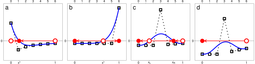
Figure 1: Gain sequence $\mathbf{d}$ (squares, dotted line; top axis), and corresponding gain function $g(x)$ (solid line; bottom axis) and phase portrait (circles, arrows) for threshold games given by (7) and (8) with $N=7$, $r=2$, $c=1$, and (a) $m=1$ (see section 4.2.1), (b) $m=N=n+1$ (see section 4.2.2), or (c) $m=4$ (see section 4.2.3). Panel d illustrates the same game as in panel c, but with $c=3$ instead of $c=1$.

It is obvious that the gain sequence $\mathbf{d}$ has no sign change when $r\leq c_{m-1}$ and that in this case defection is a dominant strategy. As illustrated in Fig. 1 and discussed below, in the other cases the sign pattern of the gain sequence depends on the location of the threshold $m$.

4.2.1 Threshold $m=1$

Threshold games with $m=1$ represent situations in which only one cooperator is required for the provision of the public good. Such games have been considered by Dugatkin (1990), Weesie and Franzen (1998), Zheng et al. (2007), and Souza et al. (2009) for the particular case of a cost sequence satisfying $c_{k}=c/(k+1)$ for some constant $c>0$, so that the cost to cooperators is inversely proportional to the total number of cooperators in the group. These authors have shown by algebraic manipulations or numerical simulations that for such games the replicator dynamics has at most one interior stable rest point. Archetti (2009) shows the same result for a cost sequence satisfying $c_{k}=c$ for some constant $c>0$.

Considering the sign pattern of the gains from switching not only recovers this result in a simpler way, but also extends it to any strictly positive cost sequence $\bm{c}$. If $r>c_{0}$, the gain sequence given in (7) has exactly one sign change and $I(\mathbf{d})=+$, so that Result 3.2.b establishes the existence of a single interior stable rest point $0<x^{*}<1$ and the instability of the trivial rest points (see Fig. 1.a). If $r\leq c_{0}$, Result 3.1.a applies. Hence, there is no interior rest point and $x=0$ is the unique stable rest point.

4.2.2 Threshold $m=n+1$

Recalling that $N=n+1$ is group size, threshold games with $m=n+1$ represent situations in which the cooperation of all group members is required to produce the public good. For the case $m=n+1=2$ and a cost sequence satisfying $0<c_{0}=c_{1}<r$, Souza et al. (2009) observe that such a threshold game corresponds to a two-player stag hunt game (Skyrms, 2004) in which both trivial rest points are stable and there is a unique, unstable interior rest point. It is easy to see that this result holds more generally. Indeed, provided that the cost sequence is strictly positive and satisfies $r>c_{n}$, the gain sequence given in (7) is characterized by $S(\mathbf{d})=1$ and $I(\mathbf{d})=-$. Then, by Result 3.2.a, it follows that the qualitative dynamics of the two-player stag hunt are recovered for every threshold game with $m=n+1$ (see Fig. 1.b). The case $r\leq c_{n}$ is covered by Result 3.1.a.

4.2.3 Threshold $1<m<n+1$

Souza et al. (2009) studied a threshold game with $1<m<n+1$ for a cost sequence of the form

$$c_{k}=\left\{\begin{array}[]{ll}c/m&\mbox{if }k<m-1\\ c/(k+1)&\mbox{if }k\geq m-1\end{array}\right.$$ (8)

for some constant $c>0$. Their main theoretical result (Souza et al., 2009, Theorem 1) uses an ingenious but rather involved argument to demonstrate that in this example there exists $\bar{c}>0$ and $0<\bar{x}<1$ such that (i) if $c<\bar{c}$, the replicator dynamics has two interior rest points $x_{\mathrm{L}}<\bar{x}<x_{\mathrm{R}}$ where $x_{\mathrm{L}}$ is unstable and $x_{\mathrm{R}}$ is stable (see Fig. 1.c), (ii) if $c=\bar{c}$, the replicator dynamics has a unique rest point $\bar{x}$ (which is unstable), and (iii) if $c>\bar{c}$, the replicator dynamics has no interior rest point (see Fig. 1.d).

In Appendix B we prove that the same result holds for any cost sequence of the form $c_{k}=c\cdot\gamma_{k}$, where the strictly positive, but otherwise arbitrary, sequence $\bm{\gamma}$ describes the shape of the cost sequence and, as in the example considered by Souza et al. (2009), $c$ shifts the level of the cost sequence. Our result follows, in essence, from two observations. The first is that for every threshold game with $1<m<n+1$ and strictly positive cost sequence satisfying $0<c_{m-1}<r$ the gain sequence has two sign changes and a negative initial sign, so that the rest points of the replicator dynamics are described by Result 4.1. The second observation is that the maximal value of the gain function $\bar{g}$ is strictly decreasing in the cost parameter $c$.

Threshold games with $1<m<n+1$ have also been considered by Bach et al. (2006), Archetti (2009), and Archetti and Scheuring (2011). These authors assume a cost sequence satisfying $c_{k}=c$ for some constant $c>0$, implying that these games fall in the class of constant cost games with sigmoid benefit functions that we discuss in Section 4.3.3.

4.2.4 Further threshold games

In economics, Höffler (1999) and Herold (2012) have studied evolutionary dynamics of threshold games which differ from the biological threshold games considered above in that cooperators pay a cost only if the threshold for the successful provision of the public good is reached. In such cases the gain sequence has the form

$$d_{k}=\left\{\begin{array}[]{ll}0&\mbox{if }k<m-1\\ r-c_{m-1}&\mbox{if }k=m-1\\ -c_{k}&\mbox{if }k>m-1\end{array}\right.$$ (9)

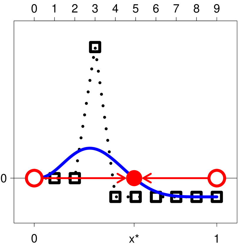
Figure 2: Gain sequence $\mathbf{d}$ (squares, dotted line; top axis), and corresponding gain function $g(x)$ (solid line; bottom axis) and phase portrait (circles, arrows) for the threshold game given by (9) with $N=10$, $r=2$, $m=4$, and $c_{k}=1/4$ for all $k\geq 3$.

and thus possesses at most one sign change (see Fig. 2). For $r>c_{m-1}$ and $1\leq m<n+1$, this gain sequence satisfies $I(\mathbf{d})=+$ and $S(\mathbf{d})=1$. Applying Result 3.2.b then yields a simple direct proof of the main result obtained by Höffler (1999, Proposition 1) and Herold (2012, Proposition 1) for this class of games, namely that there exists a unique stable interior rest point.

4.3 Constant cost games

If there exists a constant $c>0$ such that $c_{k}=c$ holds for $k=0,\ldots,n$ we say that a public goods game is a constant cost game. Such games have been studied, among others, by Motro (1991), Szathmáry (1993), Bach et al. (2006), Hauert et al. (2006), Pacheco et al. (2009), and Archetti and Scheuring (2011).

In the case of a constant cost game, equation (6) reduces to

$$d_{k}=\Delta r_{k}-c,\ k=0,1,\ldots,n.$$ (10)

It is then immediate that the gain sequence has no sign change (and hence no interior rest point) if $c\geq\max_{k=0,\ldots,n}\Delta r_{k}$ or $\min_{k=0,\ldots,n}\Delta r_{k}\geq c$ holds. It follows from Result 3.1 that in the former case $x=0$ and in the latter case $x=1$ is the unique stable rest point. In all other cases, that is whenever the inequality

$$\min_{k=0,\ldots,n}\Delta r_{k}<c<\max_{k=0,\ldots,n}\Delta r_{k}$$ (11)

holds, the gain sequence has at least one sign change.

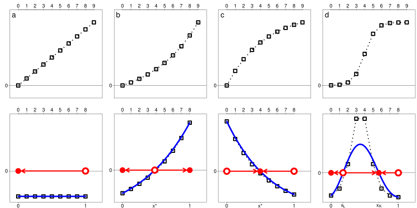
Figure 3: Examples of constant cost games with $N=n+1=9$ and $c=1/2$ for different benefit sequences. The first row shows the benefit sequence $r_{j}$; the second row shows the gain sequence $\mathbf{d}$ (squares, dotted line; top axis), and corresponding gain function $g(x)$ (solid line; bottom axis) and phase portrait (circles, arrows). (a) Linear benefits (see Section 4.3.1) with $r=5$ and $c=1$. (b) Convex benefits (see Section 4.3.2) as given by (13) with $r=5$ and $w=1.2$. (c) Concave benefits (see Section 4.3.2) as given by (13) with $r=20$ and $w=0.8$. (d) Sigmoid benefits (see Section 4.3.3) as studied by Archetti and Scheuring (2011) with $r_{j}=r/[1+\exp(-s(j-m))]$, $r=20$, $m=4$, and $s=1.5$.

In the following, we consider three different kinds of constant cost games, arising from three different assumptions on the shape of the benefit sequence: linear benefits (Section 4.3.1), convex or concave benefits (Section 4.3.2) and sigmoid benefits (Section 4.3.3). See Fig. 3 for a graphical illustration of these different constant cost games.

4.3.1 Linear benefits

The familiar linear public goods game is a constant cost game in which the benefit sequence is given by $r_{j}=jr/(n+1)$ (Sigmund, 2010). The interpretation is that $r>0$ is the amount of the public good produced by each cooperator and that this amount is split evenly among the $N=n+1$ members of the group. For such a game, we have $\Delta r_{k}=r/(n+1)$, so that the gain sequence is $d_{k}=r/(n+1)-c$, which is a constant independent of $k$. Hence $\mathbf{d}$ has no sign change. Making the standard assumption $r<(n+1)c$, we have $I(\mathbf{d})=-$, so that there are no interior rest points and $x=0$ is the unique stable rest point (see Fig. 3.a). This conclusion is, of course, well-known.

4.3.2 Convex or concave benefits

Convexity of the benefit sequence ($\Delta^{2}\bm{r}\geq\bm{0}$) indicates that the incremental benefit $\Delta r_{k}$ of a further contributor is increasing in the number of other contributors $k$ that are already present in the group. Using (10) to obtain

$$\Delta d_{k}=\Delta^{2}r_{k},\ k=0,1,\ldots,n-1,$$ (12)

it is apparent that that the gain sequence $\mathbf{d}$ is increasing. As discussed in Section 3.4.1 it follows that (11) reduces to $\Delta r_{0}<c<\Delta r_{n}$. Furthermore, if these inequalities hold, Result 3.2.a implies that there is a unique interior rest point which is unstable, whereas both trivial rest points are stable (see Fig. 3.b). Similarly, when the benefit sequence is concave ($\Delta^{2}\bm{r}\leq\bm{0}$), (11) reduces to $\Delta r_{n}<c<\Delta r_{0}$ and if these inequalities hold, Result 3.2.b implies there is a unique interior rest point which is stable, whereas both trivial rest points are unstable (see Fig. 3.c).

The argument we have just given recovers the main results from Motro (1991). A simple illustration of a constant cost game with convex or constant benefits is provided by the model of synergy and discounting considered in Hauert et al. (2006, Section 2.1). These authors consider a constant cost game with benefit function

$$r_{j}=\frac{r}{n+1}\left(1+w+\ldots w^{j-1}\right),$$ (13)

where $r>0$ and $w>0$ are parameters. For this specification we have $\Delta r_{k}=rw^{k}/(n+1)$. For $w>1$ this benefit sequence is convex, whereas for $w<1$ it is concave. The case $w=1$ is the linear public goods game. We observe that the classification obtained in Section 2.2 of Hauert et al. (2006), corresponds to the one obtained from a straightforward application of our Result 3.

4.3.3 Sigmoid benefits

A benefit sequence is sigmoid (or S-shaped) when $\Delta^{2}\bm{r}$ has exactly one sign change from $+$ to $-$, i.e. the benefit sequence is first convex, then concave. Examples of sigmoid benefit sequences are the threshold benefit sequences with $1<m<n+1$ considered in Section 4.2.3, the “benefit function with a hump” proposed in Szathmáry (1993), and the threshold-linear and logistic benefit sequences studied respectively by Pacheco et al. (2009) and Archetti and Scheuring (2011).

In this case it is immediate from (12) that the gain sequence of a constant cost game with sigmoid benefits is unimodal. Consequently, the characterization of the different types of dynamics that can arise in such games involves nothing more than inserting the values $d_{k}=\Delta r_{k}-c$ into our Result 5 (see Fig. 3.d for a particular example). The results of this exercise have been published by Archetti (2013).

Sigmoid benefit sequences generalize the benefit sequences considered in Bach et al. (2006, Proposition 7), who not only assume that $\Delta^{2}\bm{r}$ has a single sign change from $+$ to $-$, but, in addition, require $\Delta^{2}\bm{r}$ to be decreasing. Using these assumptions,  Bach et al. (2006) establish the existence of a $c^{*}>\max\{\Delta r_{0},\Delta r_{n}\}$ such that for $c<c^{*}$ the replicator dynamics has two interior rest points (the larger of which is stable), whereas for $c=c^{*}$ there is a unique (unstable) interior rest point and for $c>c^{*}$ there is none. As the gain sequence (and hence the gain function and $\bar{g}$) for constant cost games is linearly decreasing in $c$, it is immediate from Result 5 that the same conclusion obtains for all sigmoid benefit sequences.

5 Other multi-player games

Up to this point our examples have considered public goods games. Here we consider two examples of other multi-player games, illustrating how focusing on the shape of the gain sequence obviates the need for a more involved analysis. Of course, further examples could be analyzed along similar lines. For instance, it is straightforward to show that in the “shared reward dilemma” considered by Cuesta et al. (2008) the gain sequence has at most two sign changes, so that we can recover their case distinctions by applying our results.

5.1 Repeated $N$-person prisoner’s dilemma

Joshi (1987), Boyd and Richerson (1988) and van Segbroeck et al. (2012) considered a repeated $N$-person prisoner’s dilemma with two possible strategies. Reciprocators (A-strategists) contribute to the public good in the first round and then contribute in each subsequent round if at least $m$ individuals (including the focal individual) contributed in the previous move. Defectors (B-strategists) never contribute to the public good. Payoffs in each round depend on the number of contributors as in the linear public goods game considered in Section 4.3.1.

The gain sequence for this model is easily derived by considering the first round and the subsequent rounds separately. In the first round, the gain if switching from B to A is $r/(n+1)-c<0$. In each subsequent round, the gain from switching is zero if $k<m-1$ (because all players defect), $r/(n+1)-c$ if $k>m-1$ (because the other reciprocators cooperate no matter whether the focal individual contributes or not), and $mr/(n+1)-c$ if $k=m-1$ (because in this case the contribution of the focal individual in the first round is pivotal in determining the subsequent behavior of reciprocators). Setting

$$\tilde{c}=c-r/(n+1)>0,$$

and

$$\tilde{r}=(m-1)r/(n+1),$$

the gain sequence can be written as

$$d_{k}=\left\{\begin{array}[]{ll}-\tilde{c}&\mbox{if }k<m-1\\ T\tilde{r}-(T+1)\tilde{c}&\mbox{if }k=m-1\\ -(T+1)\tilde{c}&\mbox{if }k>m-1\end{array}\right.,$$ (14)

where $T>0$ denotes the expected number of rounds after the first one. From (7) and (14) it is apparent that the model is equivalent to a threshold game with (i) the benefit $T\tilde{r}$ arising if and only if at least $m$ reciprocators are present and (ii) costs given by $c_{k}=\tilde{c}$ if $k<m-1$ and $c_{k}=(T+1)\tilde{c}$ otherwise. In particular, the results for the cases $m=1$ and $m=n+1$ are identical to the ones discussed in Sections 4.2.1 and 4.2.2. Moreover, when $T\tilde{r}-(T+1)\tilde{c}$ is negative, it is immediate that the gain sequence is negative and Result 3.1.a applies.

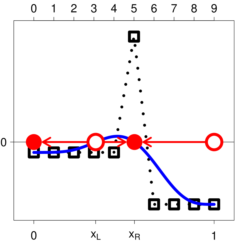
Figure 4: Gain sequence $\mathbf{d}$ (squares, dotted line; top axis), and corresponding gain function $g(x)$ (solid line; bottom axis) and phase portrait (circles, arrows) for the repeated $N$-person prisoner’s dilemma given by (14) with $N=10$, $r=7$, $c=2$, $T=5$, and $m=6$.

In the remaining case, satisfying $1<m<n+1$ and $T\tilde{r}-(T+1)\tilde{c}>0$, it follows from (14) that the only non-zero elements of $\Delta\bm{d}$ are $\Delta d_{m-2}>0$ and $\Delta d_{m-1}<0$. Consequently, the gain sequence is unimodal and Result 5 applies with $\max\{d_{0},d_{n}\}<0$ to characterize the three different possible dynamical regimes. Which of these regimes arises depends on the value of $\bar{g}=g(\hat{x})$ (see Fig. 4 for an example of the case $\bar{g}>0$). As in all applications of Results 4 and 5, a key question is whether this value can be linked to the parameters of the model.

For the parameter $T$ this question can be answered by using the linearity of the Bernstein operator $\mathcal{B}_{n}$ to write the gain function as

$$g(x)=Th(x)-\tilde{c},$$ (15)

where $h(x)=\mathcal{B}_{n}(x,\bm{e})$ and the sequence $\bm{e}$ is given by

$$e_{k}=\left\{\begin{array}[]{ll}0&\mbox{if }k<m-1\\ \tilde{r}-\tilde{c}&\mbox{if }k=m-1\\ -\tilde{c}&\mbox{if }k>m-1\end{array}\right..$$

It follows from (15) that the critical value $\hat{x}$ satisfying the first order condition $g^{\prime}(\hat{x})=0$ is independent of $T$. Further, because $I(\bm{e})=+$, it follows from the preservation of initial signs that $h(\hat{x})>0$ holds. This in turn implies from (15) that $g(\hat{x})$ is strictly increasing in $T$ and that the equation $\hat{T}=\tilde{c}/h(\hat{x})$ identifies the critical value of $T$ at which $g(\hat{x})=0$ holds. Hence, we obtain the same conclusions as van Segbroeck et al. (2012) by an application of Result 5. Namely, (i) for $T<\hat{T}$ there is no interior rest point, (ii) for $T=\hat{T}$ the replicator dynamics has a single, unstable interior rest point, and (iii) for $T>\hat{T}$ two interior rest points emerge.

5.2 Constant cost game with different benefit sequences for cooperators and defectors

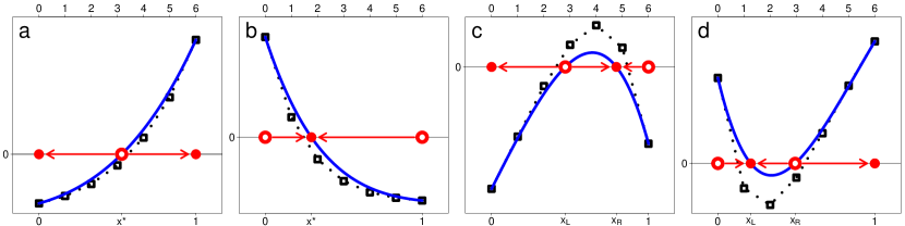
Figure 5: Gain sequence $\mathbf{d}$ (squares, dotted line; top axis), and corresponding gain function $g(x)$ (solid line; bottom axis) and phase portrait (circles, arrows) of the game considered in Section 5.2 for $N=7$ and different values of the parameters $w$, $v$, $r$ and $c$. (a) $w=1.3$, $v=1.2$, $r=1$, $c=3$. (b) $w=0.6$, $v=0.57$, $r=2$, $c=1$. (c) $w=1.3$, $v=1.4$, $r=2$, $c=3.4$. (d) $w=0.75$, $v=0.6$, $r=1.55$, $c=1.25$.

Hauert et al. (2006, Section 2.3.2) consider an interesting extension of constant cost games by allowing for the possibility that cooperators and defectors might obtain different benefits, say $r^{A}_{j}$ and $r^{B}_{j}$, when there are $j$ cooperators in the group (see Fig. 5). The counterpart to (12) is then $\Delta d_{k}=\Delta r^{A}_{k+1}-\Delta r^{B}_{k}$. For the particular choice of benefit sequences in Hauert et al. (2006), given by (13) for $r^{A}_{j}$ and

$$r^{B}_{j}=\frac{r}{n+1}\left(1+v^{1}+\ldots v^{j-1}\right),$$

this reduces to

$$\Delta d_{k}=\frac{r}{n+1}\left(w^{k+1}-v^{k}\right),$$ (16)

where $r>0$, $v>0$ and $w>0$ are parameters and $N=n+1$ is group size.

Hauert et al. (2006) state that “only $v=w$ allows for an analytical solution […] but in general there are […] up to $N-1$ equilibria [rest points] in $(0,1)$.” Here we refine this statement and show that, as conjectured by Cuesta et al. (2007), the maximum number of interior rest points is two independently of group size. To do so, we observe that $\Delta d_{k}>0$ holds if and only if

$$w>\left(\frac{v}{w}\right)^{k}.$$

Since the right side of this inequality is monotonic in $k$, equation (16) implies the following, exhaustive case distinction:

1. if $w\geq 1$ and $w^{n}\geq v^{n-1}$ holds, then the gain sequence is increasing and there is at most one interior rest point (see Fig. 5.a).

2. if $w\leq 1$ and $w^{n}\leq v^{n-1}$ holds, then the gain sequence is decreasing and there is at most one interior rest point (see Fig. 5.b).

3. if $w>1$ and $w^{n}<v^{n-1}$ holds, then the gain sequence is unimodal and there are at most two interior rest points (see Fig. 5.c).

4. if $w<1$ and $w^{n}>v^{n-1}$ holds, then the gain sequence is anti-unimodal and there are at most two interior rest points (see Fig. 5.d).

6 Discussion

Bernstein polynomials were first proposed more than a century ago by Bernstein (1912) in order to provide a constructive proof of Weierstrass’s approximation theorem (DeVore and Lorentz, 1993). More recently, and because of their many shape-preserving properties, polynomials in Bernstein form have proven extremely useful in the field of computer aided geometric design (Yamaguchi and Yamaguchi, 1988; Farin and Hoschek, 2002). Here we have made the case for utilizing the shape-preserving properties of Bernstein polynomials in the analysis of multi-player matrix games. In particular, we have used these properties to show how key insights into the evolutionary dynamics of multi-player matrix games can be obtained from studying the sign pattern of the gains from switching.

The properties of Bernstein polynomials we have used in this paper are certainly not the only ones of relevance for the theoretical analysis of collective action problems. For instance, both the effects of changes in the group size (studied previously in Motro, 1991) and the group size distribution (studied previously in Peña, 2012) on the evolutionary dynamics can be analyzed by making use of the theory of polynomials in Bernstein form. Our methods can also be extended to structured populations and used to analyze multi-player matrix games played between relatives.

Appendix A Proof of Result 1

We show the result $I(g)=I(\mathbf{d})$; the argument that the final signs coincide is analogous. Using the derivative property of polynomials in Bernstein form (cf. equation (5)) recursively, for $0\leq m\leq n$ the $m$-th derivative of the gain function can be written as (Farouki, 2012)

$$g^{(m)}(x)=n(n-1)\ldots(n-m+1)\mathcal{B}_{n-m}\left(x;\Delta^{m}\mathbf{d}\right),$$ (A.1)

where (with the obvious iterative definition) $\Delta^{m}\mathbf{d}$ is the $m$-th forward difference of the sequence $\mathbf{d}$. Evaluating (A.1) at $x=0$ we obtain

$$g^{(m)}(0)=n(n-1)\ldots(n-m+1)\Delta^{m}d_{0}.$$ (A.2)

Now, let $\ell$ be the lowest index $k$ such that $d_{\ell}\not=0$. Then $\Delta^{m}d_{0}=0$ holds for all $m<\ell$ and $\Delta^{\ell}d_{0}=d_{\ell}$. Equation (A.2) then implies that $g^{(m)}(0)=0$ for all $m<\ell$ and that the sign of $g^{(\ell)}(0)$ coincides with the sign of $d_{\ell}$ which, by definition, is the initial sign of $\mathbf{d}$. A standard Taylor-series argument as given in Bach et al. (2006, Proof of Proposition 4) demonstrates that the initial sign of $g$ coincides with the sign of $d_{\ell}$, finishing the proof.

Appendix B Proof of the generalization of Theorem 1 from Souza et al. (2009)

For any $c\geq 0$ let

$$g(x,c)=\sum_{k=0}^{n}\binom{n}{k}x^{k}(1-x)^{n-k}d_{k}(c),$$ (B.1)

where

$$d_{k}(c)=\left\{\begin{array}[]{ll}-c\gamma_{k}&\mbox{if }k<m-1\\ r-c\gamma_{m-1}&\mbox{if }k=m-1\\ -c\gamma_{k}&\mbox{if }k>m-1\end{array}\right.$$ (B.2)

and $\bm{\gamma}=(\gamma_{0},\ldots,\gamma_{n})$ is a given, strictly positive sequence. Let $\bar{g}(c)=\max_{0\leq x\leq 1}g(x,c)$ denote the corresponding maximal value of the gain function.

For $0<c<r/\gamma_{m-1}$ the gain sequence given in (B.2) satisfies $I(\mathbf{d}(c))=-$ and $S(\mathbf{d}(c))=2$, so that the rest points of the replicator dynamics are described by Result 4.1.

From (B.1) and (B.2) the function $g(x,c)$ is continuous. From the maximum theorem (Sundaram, 1996, Theorem 9.14) this ensures continuity of $\bar{g}(c)$. Because all the Bernstein coefficients $d_{k}(c)$ are strictly decreasing in $c$, every of the summands appearing in (B.1) is strictly decreasing in $c$, implying that $g(x,c)$ is strictly decreasing in $c$. This monotonicity property obviously carries over to $\bar{g}(c)$.

Consider the Bernstein coefficients as given in (B.2). If $c=0$, the only non-zero coefficient is $d_{m-1}(0)=r>0$. It is then immediate from (B.1) that $g(x,0)>0$ holds for all $0<x<1$, ensuring $\bar{g}(0)>0$. If $c=r/\gamma_{m-1}$, we have $d_{k}(c)\leq 0$ with strict inequality holding in all cases but $k=m-1$. From (B.1) this implies $g(x,r/\gamma_{m-1})<0$ for all $0\leq x\leq 1$, ensuring $\bar{g}(r/\gamma_{m-1})<0$.

Because $\bar{g}(0)>0$ and $\bar{g}(r/\gamma_{m-1})<0$ hold and $\bar{g}(c)$ is continuous the intermediate value theorem implies that there exists $0<\bar{c}<r/\gamma_{m-1}$ satisfying $\bar{g}(\bar{c})=0$. By monotonicity of $\bar{g}(c)$ it follows that $\bar{g}(c)<0$ holds for $c>\bar{c}$ and $\bar{g}(c)>0$ holds for $c<\bar{c}$. The generalized version of Theorem 1 in Souza et al. (2009) then follows from our Result 4.1 – except that it remains to establish the existence of $0<\bar{x}<1$ such that the interior rest points satisfy $x_{\mathrm{L}}<\bar{x}<x_{\mathrm{R}}$ for all $0<c<\bar{c}$. Towards this end let $\bar{x}$ be a solution to the problem $\max_{0\leq x\leq 1}g(x,\bar{c})$. As $g(0,\bar{c})<0$ and $g(1,\bar{c})<0$ holds, we have $0<\bar{x}<1$. As $g(x,c)$ is strictly decreasing in $c$, we have $g(\bar{x},c)>0$ for all $0<c<\bar{c}$. In conjunction with $g(0,c)<0$ and $g(1,c)<0$ this implies that $g(x,c)$ has at least one root in the interval $(0,\bar{x})$ and at least one root in the interval $(\bar{x},1)$.

References

- Archetti (2009) Archetti, M., 2009. The volunteer’s dilemma and the optimal size of a social group. Journal of Theoretical Biology 261 (3), 475–480.
- Archetti (2013) Archetti, M., 2013. Evolutionary game theory of growth factor production: implications for tumour heterogeneity and resistance to therapies. British Journal of Cancer 109 (4), 1056–1062.
- Archetti and Scheuring (2011) Archetti, M., Scheuring, I., 2011. Coexistence of cooperation and defection in public goods games. Evolution 65 (4), 1140–1148.
- Bach et al. (2006) Bach, L., Helvik, T., Christiansen, F., 2006. The evolution of n-player cooperation–threshold games and ESS bifurcations. Journal of Theoretical Biology 238 (2), 426–434.
- Bernstein (1912) Bernstein, S., 1912. Démonstration du théoreme de Weierstrass fondée sur le calcul des probabilités. Comm. Soc. Math. Kharkov 13 (2), 1–2.
- Boyd and Richerson (1988) Boyd, R., Richerson, P. J., 1988. The evolution of reciprocity in sizable groups. Journal of Theoretical Biology 132 (3), 337–356.
- Broom et al. (1997) Broom, M., Cannings, C., Vickers, G., 1997. Multi-player matrix games. Bulletin of Mathematical Biology 59 (5), 931–952.
- Broom and Rychtář (2013) Broom, M., Rychtář, J., 2013. Game-theoretical models in biology. Chapman and Hall, New York, NY.
- Brown et al. (1981) Brown, L. D., Johnstone, I. M., MacGibbon, K. B., 1981. Variation diminishing transformations: A direct approach to total positivity and its statistical applications. Journal of the American Statistical Association, 824–832.
- Bulmer (1994) Bulmer, M., 1994. Theoretical Evolutionary Ecology. Sinauer Associates, Sunderland, Massachusetts.
- Bulmer and Parker (2002) Bulmer, M. G., Parker, G. A., 2002. The evolution of anisogamy: A game-theoretic approach. Proceedings of the Royal Society of London Series B-Biological Sciences 269, 2381–2388.
- Clark (1984) Clark, A., 1984. Elements of abstract algebra. Courier Dover Publications, New York, NY.
- Clark and Mangel (1986) Clark, C. W., Mangel, M., 1986. The evolutionary advantages of group foraging. Theoretical Population Biology 30, 45–75.
- Comins et al. (1980) Comins, H. N., Hamilton, W. D., May, R. M., 1980. Evolutionarily stable dispersal strategies. Journal of Theoretical Biology 82, 205–230.
- Cressman (2003) Cressman, R., 2003. Evolutionary dynamics and extensive form games. MIT Press, Cambridge, MA.
- Cuesta et al. (2008) Cuesta, J., Jiménez, R., Lugo, H., Sánchez, A., 2008. The shared reward dilemma. Journal of Theoretical Biology 251 (2), 253–263.
- Cuesta et al. (2007) Cuesta, J. A., Jiménez, R., Lugo, H., Sánchez, A., 2007. Rewarding cooperation in social dilemmas. UC3M Working papers. Economics 07-27, Universidad Carlos III de Madrid. Departamento de Economía.
- DeVore and Lorentz (1993) DeVore, R. A., Lorentz, G. G., 1993. Constructive Approximation. Springer-Verlag, Berlin, Germany.
- Dieckmann and Law (1996) Dieckmann, U., Law, R., 1996. The dynamical theory of coevolution: a derivation from stochastic ecological processes 34 (5-6), 579–612.
- Diekmann (1985) Diekmann, A., 1985. Volunteer’s dilemma. The Journal of Conflict Resolution 29 (4), 605–610.
- Dugatkin (1990) Dugatkin, L. A., 1990. N-person games and the evolution of co-operation: A model based on predator inspection in fish. Journal of Theoretical Biology 142 (1), 123–135.
- Eshel (1996) Eshel, I., 1996. On the changing concept of evolutionary population stability as a reflection of a changing point of view in the quantitative theory of evolution. Journal of Mathematical Biology 34, 485–510.
- Farin and Hoschek (2002) Farin, G., Hoschek, J., 2002. Handbook of computer aided geometric design. North Holland, Amsterdam, Netherlands.
- Farouki (2012) Farouki, R. T., 2012. The Bernstein polynomial basis: A centennial retrospective. Computer Aided Geometric Design 29 (6), 379–419.
- Foster (2004) Foster, K. R., 2004. Diminishing returns in social evolution: the not-so-tragic commons. Journal of Evolutionary Biology 17, 1058–1072.
- Frank (1987) Frank, S. A., 1987. Individual and population sex allocation patterns. Theoretical Population Biology 31, 47–74.
- Frank (1995) Frank, S. A., 1995. Mutual policing and repression of competition in the evolution of cooperative units. Nature 377, 520–522.
- Gokhale and Traulsen (2010) Gokhale, C. S., Traulsen, A., 2010. Evolutionary games in the multiverse. Proceedings of the National Academy of Sciences 107 (12), 5500–5504.
- Hardin (1982) Hardin, R., 1982. Collective action. The John Hopkins Press for Resources for the Future, Baltimore, Maryland.
- Hauert et al. (2006) Hauert, C., Michor, F., Nowak, M. A., Doebeli, M., 2006. Synergy and discounting of cooperation in social dilemmas. Journal of Theoretical Biology 239 (2), 195–202.
- Herold (2012) Herold, F., 2012. Carrot or stick? The evolution of reciprocal preferences in a haystack model. The American Economic Review 102 (2), 914–940.
- Hofbauer and Sigmund (1998) Hofbauer, J., Sigmund, K., 1998. Evolutionary Games and Population Dynamics. Cambridge University Press, Cambridge, UK.
- Höffler (1999) Höffler, F., 1999. Some play fair, some don’t: Reciprocal fairness in a stylized principal–agent problem. Journal of economic behavior & organization 38 (1), 113–131.
- Joshi (1987) Joshi, N., 1987. Evolution of cooperation by reciprocation within structured demes. Journal of Genetics 66 (1), 69–84.
- Kirkpatrick and Rousset (2005) Kirkpatrick, M., Rousset, F., 2005. Wright meets AD: not all landscapes are adaptive. Journal of Evolutionary Biology 18 (5), 1166–1169.
- Kurokawa and Ihara (2009) Kurokawa, S., Ihara, Y., 2009. Emergence of cooperation in public goods games. Proceedings of the Royal Society B: Biological Sciences 276 (1660), 1379–1384.
- Lorentz (1986) Lorentz, G. G., 1986. Bernstein polynomials. Chelsea Publishing Company, New York, NY.
- Maynard Smith (1982) Maynard Smith, J., 1982. Evolution and the theory of games. Cambridge University Press, Cambridge, UK.
- Motro (1991) Motro, U., 1991. Co-operation and defection: Playing the field and the ESS. Journal of Theoretical Biology 151 (2), 145–154.
- Otto and Day (2007) Otto, S. P., Day, T., 2007. A Biologist’s Guide to Mathematical Modeling in Ecology and Evolution. Princeton University Press, Princeton, NJ.
- Pacheco et al. (2009) Pacheco, J. M., Santos, F. C., Souza, M. O., Skyrms, B., 2009. Evolutionary dynamics of collective action in n-person stag hunt dilemmas. Proceedings of the Royal Society B: Biological Sciences 276 (1655), 315–321.
- Peña (2012) Peña, J., 2012. Group-size diversity in public goods games. Evolution 66 (3), 623–636.
- Rousset (2004) Rousset, F., 2004. Genetic Structure and Selection in Subdivided Populations. Princeton University Press, Princeton, NJ.
- Sigmund (2010) Sigmund, K., 2010. The calculus of selfishness. Princeton University Press, Princeton, NJ.
- Skyrms (2004) Skyrms, B., 2004. The stag hunt and the evolution of social structure. Cambridge University Press, Cambridge, UK.
- Souza et al. (2009) Souza, M. O., Pacheco, J. M., Santos, F. C., 2009. Evolution of cooperation under n-person snowdrift games. Journal of Theoretical Biology 260 (4), 581–588.
- Sugden (1986) Sugden, R., 1986. The economics of rights, co-operation and welfare. Blackwell, Oxford, UK.
- Sundaram (1996) Sundaram, R. K., 1996. A first course in optimization theory. Cambridge University Press, Cambridge, UK.
- Szathmáry (1993) Szathmáry, E., 1993. Co-operation and defection: Playing the field in virus dynamics. Journal of Theoretical Biology 165 (3), 341–356.
- Taylor and Ward (1982) Taylor, M., Ward, H., 1982. Chickens, whales, and lumpy goods: alternative models of public-goods provision. Political Studies 30 (3), 350–370.
- Taylor and Jonker (1978) Taylor, P. D., Jonker, L. B., 1978. Evolutionary stable strategies and game dynamics. Mathematical Biosciences 40, 145–156.
- van Segbroeck et al. (2012) van Segbroeck, S., Pacheco, J. M., Lenaerts, T., Santos, F. C., 2012. Emergence of fairness in repeated group interactions. Phys. Rev. Lett. 108, 158104.
- Vincent and Brown (2005) Vincent, T. L., Brown, J. S., 2005. Evolutionary game theory, natural selection, and Darwinian dynamics. Cambridge University Press, Cambridge, UK.
- Weesie and Franzen (1998) Weesie, J., Franzen, A., 1998. Cost sharing in a volunteer’s dilemma. Journal of Conflict Resolution 42 (5), 600–618.
- Weibull (1995) Weibull, J. W., 1995. Evolutionary game theory. The MIT press, Cambridge, MA.
- Yamaguchi and Yamaguchi (1988) Yamaguchi, F., Yamaguchi, F., 1988. Curves and surfaces in computer aided geometric design. Springer-Verlag Berlin, Berlin, Germany.
- Zheng et al. (2007) Zheng, D. F., Yin, H. P., Chan, C. H., Hui, P. M., 2007. Cooperative behavior in a model of evolutionary snowdrift games with n-person interactions. EPL (Europhysics Letters) 80 (1), 18002.