Fluctuating hydrodynamics of multi-species, non-reactive mixtures

Abstract

In this paper we discuss the formulation of the fluctuating Navier-Stokes (FNS) equations for multi-species, non-reactive fluids. In particular, we establish a form suitable for numerical solution of the resulting stochastic partial differential equations. An accurate and efficient numerical scheme, based on our previous methods for single species and binary mixtures, is presented and tested at equilibrium as well as for a variety of non-equilibrium problems. These include the study of giant nonequilibrium concentration fluctuations in a ternary mixture in the presence of a diffusion barrier, the triggering of a Rayleigh-Taylor instability by diffusion in a four-species mixture, as well as reverse diffusion in a ternary mixture. Good agreement with theory and experiment demonstrates that the formulation is robust and can serve as a useful tool in the study of thermal fluctuations for multi-species fluids. The extension to include chemical reactions will be treated in a sequel paper.

I Introduction

Since the pioneering work of Einstein and Smoluchowski on Brownian motion it has been clear that hydrodynamic fluctuations are essential in the study of fluid dynamics at mesoscopic scales. In fact, fluctuations play an important role in many physical, chemical, and biological processes, ranging from phase separation to ion transport in cells. For example, high-fidelity molecular simulations reveal that thermal fluctuations significantly affect fluid mixing, both in simple diffusion Donev_11 ; DiffusionRenormalization and in the Rayleigh-Taylor instability Kadau_04 ; Kadau_07 . The accurate modeling of droplets in nanojets Moseler_00 ; Eggers_02 and lipid bilayer membranes Atzberger2013A ; Atzberger2013B necessitate the inclusion of hydrodynamic fluctuations. Chemical processes, including combustion and explosive detonation, also depend strongly on spontaneous thermal fluctuations Nowakowski_03 ; Lemarchand_04 . Finally, the manifestation of hydrodynamic fluctuations is not restricted to mesoscale phenomena. Laboratory experiments involving gases, liquids or crystals demonstrate that, away from equilibrium, thermal fluctuations lead to large-scale structures, the so-called “giant fluctuation” effect Vailati_97 ; Vailati_98 ; Vailati_11 ; Yuk_12 .

As an extension of conventional hydrodynamic theory, fluctuating hydrodynamics incorporates spontaneous thermal fluctuations in a fluid by adding stochastic flux terms to the deterministic fluid equations Zarate_07 . These noise terms are white in space and time and are formulated using fluctuation-dissipation relations to yield the equilibrium covariances of the fluctuations. This construction was first introduced by Landau and Lifshitz Landau_59 for a single component fluid. Fox and Uhlenbeck Fox_70 ; Fox_70a provide theoretical derivations of the fluctuation terms from perspectives of Brownian motion and the Boltzmann equation. Numerous extensions of the theory have been developed, such as to Extended Thermodynamics Ikoma20112601 and plasma dynamics PhysRevE.83.015401 .

The generalization of fluctuating hydrodynamics to binary mixtures was first presented by Cohen et al. Cohen_71 and by Law and Nieuwoudt Law_89 ; Nieuwoudt_90 . Multicomponent gaseous systems are discussed within the GENERIC framework in the work of Ottinger Ottinger_09 . The standard fluctuating hydrodynamics theory for (thermo)diffusion in binary mixtures (see, for example, Ortiz de Zarate and Senger Zarate_07 ) has recently been extended to non-ideal ternary mixtures in thermodynamic equilibrium by Ortiz de Zarate et al. TernaryEquilibriumFluct .

Early work on numerical methods for the linearized fluctuating Navier-Stokes equations was performed by Garcia et al. Garcia_87 ; Garcia_87a . More recently, we developed accurate and robust numerical techniques for the full nonlinear system of equations Bell_07 ; Bell_10 ; Donev_10 ; Balboa2012 . In this paper, we extend to multicomponent systems the algorithm developed for binary gas mixtures by Bell et al. Bell_10 and subsequently improved by Donev et al. Donev_10 .

There are three reasons why this extension multi-species fluids is significant: First, it allows us to consider interesting, realistic chemical reactions, which will be the treated in a subsequent paper. Second, the majority of microscopic systems of interest (and certainly all biological systems) have negligible gradients of velocity and temperature. The dominant mechanism for non-equilibrium entropy production in these systems is from gradients of chemical potential (i.e., concentration gradients). Third, there are interesting interaction effects due to coupling of diffusion among the species. In a single species fluid, the (deterministic) thermodynamic fluxes are always in the direction of their conjugate thermodynamic force (e.g., heat flux is always from hot to cold). For a binary mixture there is an interaction between concentration and temperature (e.g., heat flux due to a concentration gradient); however, this coupling is typically weak. As we show in two examples in Section IV, diffusion barriers (zero concentration flux in the presence of a concentration gradient) and reverse diffusion (concentration flux from low to high concentration) can occur in multi-species mixtures (see for instance Duncan and Toor DuncanToor ). Giant fluctuations in binary mixtures out of thermodynamic equilibrium have been studied for a long time, and here we demonstrate that the coupling between the diffusive fluxes for different species also induces long-ranged correlations between the concentrations of different species.

The paper is organized as follows: The mathematical formulation is summarized in Section II, and the numerical scheme in Section III. Computational results validating the methodology are presented in Section IV along with examples illustrating its capabilities. Conclusions and directions for future work are discussed in Section V.

II Theory

In this section, we summarize the mathematical formulation of the full multi-component, fluctuating Navier-Stokes (FNS) equations and establish the elements needed to develop a suitable numerical method for the resulting stochastic partial differential equations. Our formulation of species diffusion is based on classical treatments, such as in DM_63 ; BirdStewartLightfoot_06 ; NewIrrevThermoBook . We want to be able to utilize existing software for computing transport properties of realistic gases such as the EGLIB package EGLIB commonly used in the reacting flow community. Consequently, we will adopt the notation given by Giovangigli Giovangigli_99 . The formulation is general with the specific case of ideal gas mixtures treated in Section II.4.

II.1 Multicomponent Hydrodynamic Equations

The species density, momentum and energy equations of hydrodynamics are given by

$$\frac{\partial}{\partial t}\left(\rho_{k}\right)+{\bf\nabla}\cdot\left(\rho_{k}{\bf v}\right)+{\bf\nabla}\cdot{\bm{\mathcal{F}}}_{k}=0,$$ (1)

$$\frac{\partial}{\partial t}\left(\rho{\bf v}\right)+{\bf\nabla}\cdot\left[\rho{\bf v}{\bf v}^{T}+p\mathbf{I}\right]+{\bf\nabla}\cdot{\bm{\Pi}}=\rho{\bf g},$$ (2)

$$\frac{\partial}{\partial t}\left(\rho E\right)+{\bf\nabla}\cdot\left[(\rho E+p){\bf v}\right]+{\bf\nabla}\cdot\left[{\bm{\mathcal{Q}}}+\bm{\Pi}\cdot{\bf v}\right]=\rho{\bf v\cdot g},$$ (3)

where $\rho_{k}$, ${\bf v}$, $p$, ${\bf g}$ and $E$ denote, respectively, the mass density for species $k$, fluid velocity, pressure, gravitational acceleration, and total specific energy for a mixture with $N_{s}$ species ($k=1,\ldots N_{s}$). Note that $\mathbf{v}\mathbf{v}^{T}$ is a (tensor) outer product with $T$ indicating transpose and $\mathbf{I}$ is the identity tensor (i.e., ${\bf\nabla}\cdot p\mathbf{I}={\bf\nabla}p$). Transport properties are given in terms of the species diffusion flux, ${\bm{\mathcal{F}}}$, viscous tensor, ${\bm{\Pi}}$, and heat flux, ${\bm{\mathcal{Q}}}$. For Newtonian fluids, the deterministic viscous tensor is,

$${\bm{\Pi}}=-\eta\left(\nabla\mathbf{v}+(\nabla\mathbf{v})^{T}\right)-\left(\kappa-\frac{2}{3}\eta\right)\mathbf{I}\left({\bf\nabla}\cdot{\bf v}\right),$$ (4)

where $\eta$ and $\kappa$ are the shear and bulk viscosity, respectively.

Exact mass conservation requires that the species diffusion flux satisfies the constraint,

$$\sum_{k=1}^{N_{s}}\bm{\mathcal{F}}_{k}=0,$$ (5)

so that summing the species equations gives the continuity equation.

$$\frac{\partial}{\partial t}\rho+{\bf\nabla}\cdot\left(\rho{\bf v}\right)=0,$$ (6)

where the total density $\rho=\sum_{k=1}^{N_{s}}\rho_{k}$. The mass fraction of the $k$-th species is denoted by $Y_{k}=\rho_{k}/\rho$ with $\sum_{k=1}^{N_{s}}Y_{k}=1$.

In fluctuating hydrodynamics, we augment the fluxes in (1)-(3) by adding a zero-mean stochastic flux to the deterministic flux. For example, the viscous tensor becomes ${\bm{\Pi}}+\widetilde{\bm{\Pi}}$ where $\langle\widetilde{\bm{\Pi}}\rangle=0$ with $\langle\,\rangle$ denoting a suitably defined ensemble average. The stochastic viscous flux tensor is a Gaussian random field that can be written as Landau_59 ; Espanol1998

$$\widetilde{\bm{\Pi}}(\mathbf{r},t)=\sqrt{2k_{B}T\eta}\;\widetilde{\mathcal{Z}}^{v}+\left(\sqrt{\frac{k_{B}\kappa T}{3}}-\sqrt{\frac{2k_{B}\eta T}{3}}\right)\text{Tr}(\widetilde{\mathcal{Z}}^{v}),$$ (7)

where $k_{B}$ is Boltzmann’s constant, $T$ is temperature and $\widetilde{\mathcal{Z}}^{v}=\left(\mathcal{Z}^{v}+(\mathcal{Z}^{v})^{T}\right)/\sqrt{2}$ is a symmetric Gaussian random tensor field. (The $\sqrt{2}$ in the denominator accounts for the variance reduction from averaging.) Here $\mathcal{Z}^{v}$ is a white-noise random Gaussian tensor field; i.e.,

$$\langle\mathcal{Z}^{v}_{\alpha\beta}(\mathbf{r},t)\mathcal{Z}^{v}_{\gamma\delta}(\mathbf{r}^{\prime},t^{\prime})\rangle=\delta_{\alpha\gamma}\delta_{\beta\delta}\,\delta(\mathbf{r}-\mathbf{r}^{\prime})\,\delta(t-t^{\prime})\;\;.$$

II.2 Stochastic Diffusion and Heat Fluxes

The formulation of the multi-species stochastic diffusion and heat fluxes is complicated by the couplings among the species fluxes (cross-diffusion effects) and by the thermal diffusion contribution (Soret and Dufour effects). The starting point for determining these fluxes is the entropy production for a mixture, as formulated by de Groot and Mazur DM_63 and by Kuiken NewIrrevThermoBook , which establishes the form of the thermodynamic forces and fluxes. We then use the fluctuation-dissipation principle to formulate the corresponding noise terms. Here we only need to consider the contributions of the heat flux and mass diffusion fluxes to entropy production. The entropy production also has a contribution due to the stress tensor, however, due to the Curie symmetry principle DM_63 , fluxes and thermodynamic forces of different tensorial character do not couple. As such, the stochastic flux in the momentum equation is the same as for a single species fluid, as given by (7).

The entropy production for a multi-component mixture at rest, in the absence of external forces  and chemistry, is given by DM_63 :

$$\mathfrak{v} = -\frac{1}{T^{2}}\bm{\mathcal{Q}}^{\prime}\cdot\nabla T-\frac{1}{T}\sum_{i=1}^{N_{s}}\bm{\mathcal{F}}_{i}\cdot\nabla_{T}\mu_{i}$$ (8)

$$= -\frac{1}{T^{2}}\bm{\mathcal{Q}}^{\prime}\cdot\nabla T-\frac{1}{T}\sum_{i=1}^{N_{s}-1}\bm{\mathcal{F}}_{i}\cdot\nabla_{T}\left(\mu_{i}-\mu_{N_{s}}\right),$$ (9)

where $\mu_{i}$ is the chemical potential per unit mass of species $i$ and

$$\bm{\mathcal{Q}}^{\prime}=\bm{\mathcal{Q}}-\sum_{k=1}^{N_{s}}h_{k}\bm{\mathcal{F}}_{k}=\bm{\mathcal{Q}}-\sum_{k=1}^{N_{s}-1}(h_{k}-h_{N_{s}})\bm{\mathcal{F}}_{k},$$ (10)

where $h_{k}$ is the specific enthalpy of the $k^{th}$ component (see discussion in II.4). In other words, $\bm{\mathcal{Q}}^{\prime}$ is the part of the heat flux that is not associated with mass diffusion. Here, $\nabla_{T}$ is a gradient derivative taken holding temperature fixed, that is,

$$\nabla_{T}\;\mu_{i}(p,T,X_{1},\ldots,X_{N_{s}-1})=\nabla\mu_{i}-\left(\frac{\partial\mu_{i}}{\partial T}\right)_{p,X_{1},\ldots,X_{N_{s}-1}}\,\nabla T,$$

where $X_{k}=n_{k}/\sum_{j=1}^{N_{s}}n_{j}$ are mole fractions, and $n_{k}$ are number densities. The mole fraction for species $k$ is given in terms of the mass fractions by $X_{k}=({\overline{m}}/{m_{k}})Y_{k}$, where $m_{k}$ is the mass of a molecule of that species, and $\overline{m}=\left(\sum_{k=1}^{N_{s}}Y_{k}/m_{k}\right)^{-1}$ is the mixture-averaged molecular weight NewIrrevThermoBook . Note that only $N_{s}-1$ of the mass or mole fractions are independent.

The general form of the phenomenological laws expresses the fluxes as linear combinations of thermodynamics forces, written in matrix form as

$$\bar{\mathbf{J}}=\bar{\bm{\mathfrak{L}}}\bar{\mathbf{X}}\qquad\mathrm{where}\qquad\mathfrak{v}=\bar{\mathbf{J}}^{T}\bar{\mathbf{X}}=\bar{\mathbf{X}}^{T}\bar{\bm{\mathfrak{L}}}^{T}\bar{\mathbf{X}}.$$

Here we use an overbar to denote the system expressed in terms of the first $N_{s}-1$ species. From (9) the fluxes $\bar{\mathbf{J}}$ and the thermodynamics forces $\bar{\mathbf{X}}$ are given by

$$\bar{\mathbf{J}}=\begin{bmatrix}\bar{\bm{\mathcal{F}}}\\ \bm{\mathcal{Q}}^{\prime}\end{bmatrix}\qquad\mathrm{and}\qquad\bar{\mathbf{X}}=\begin{bmatrix}-\frac{1}{T}\nabla_{T}(\mu_{i}-\mu_{N_{s}})\\ -\frac{1}{T^{2}}\nabla T\end{bmatrix}$$

respectively, where $\bar{\bm{\mathcal{F}}}=[\bm{\mathcal{F}}_{1},\ldots,\bm{\mathcal{F}}_{N_{s}-1}]^{T}$ is a vector of $N_{s}-1$ independent species mass fluxes. By Onsager reciprocity the matrix of phenomenological coefficients is symmetric so we can write $\bar{\bm{\mathfrak{L}}}$ as

$$\bar{\bm{\mathfrak{L}}}=\begin{bmatrix}{\bar{\mathbf{L}}}&\bar{\mathbf{l}}\\ {\bar{\mathbf{l}}}^{T}&\ell\end{bmatrix}\;\;\;,$$

where $\bar{\mathbf{L}}$ is a symmetric $N_{s}-1\times N_{s}-1$ matrix that depends on the multicomponent flux diffusion coefficients, $\bar{\mathbf{l}}$ is an $N_{s}-1$ component vector that depends on the thermal diffusion coefficients, and the scalar $\ell$ depends on the partial thermal conductivity (see II.4).

Before discussing the form of the noise terms we will first recast $\bar{\bm{\mathfrak{L}}}$ in a slightly different form. This form will facilitate comparison with the continuum transport literature (e.g., Giovangigli_99 ) and lead to a more efficient numerical algorithm. We introduce

$$\bar{\xi}=\bar{\mathbf{L}}^{-1}\bar{\mathbf{l}}\qquad\mathrm{and}\qquad\zeta=\ell-\bar{\xi}^{T}\bar{\mathbf{L}}\bar{\xi}$$

so that

$${\bar{\bm{\mathfrak{L}}}}=\begin{bmatrix}{\bar{\mathbf{L}}}&{\bar{\mathbf{L}}\bar{\xi}}\\ {\bar{\xi}^{T}{\bar{\mathbf{L}}}}&\zeta+\bar{\xi}^{T}{\bar{\mathbf{L}}}\bar{\xi}\end{bmatrix}.$$ (11)

It is important to point out that this construction works even when $\bar{\mathbf{L}}$ is not invertible, which happens when some of the species are not present. This is because $\bar{\xi}$ is always in the range of $\bar{\mathbf{L}}$.

We now want to establish the form of the stochastic fluxes in the fluctuating hydrodynamic equations. Since the fluxes are white in space and time we can write them in the form

$$\tilde{\bar{\mathbf{J}}}_{\alpha}=\bar{\mathcal{B}}\bar{\mathcal{Z}}^{(\alpha)}\qquad\mathrm{where}\qquad\widetilde{\bar{\mathbf{J}}}_{\alpha}=\begin{bmatrix}\widetilde{\bar{\bm{\mathcal{F}}}}_{\alpha}\\ \widetilde{\bm{\mathcal{Q}}}^{\prime}_{\alpha}\end{bmatrix}\qquad\mathrm{and}\qquad\bar{\mathcal{Z}}^{(\alpha)}=\begin{bmatrix}\bar{\mathcal{Z}}^{(\bm{\mathcal{F}};\alpha)}\\ {\mathcal{Z}}^{(\bm{\mathcal{Q}}^{\prime};\alpha)}\end{bmatrix}$$

where $\alpha=x,y,z$ denotes spatial direction and $\bar{\mathcal{Z}}^{(\bm{\mathcal{F}};\alpha)}=[\bar{\mathcal{Z}}^{(1;\alpha)},\ldots,\bar{\mathcal{Z}}^{(N_{s}-1;\alpha)}]^{T}$ is a vector of independent Gaussian white noise terms, that is,

$$\langle\bar{\mathcal{Z}}^{(i;\alpha)}(\mathbf{r},t)\bar{\mathcal{Z}}^{(j;\beta)}(\mathbf{r}^{\prime},t^{\prime})\rangle = \delta_{ij}\,\delta_{\alpha\beta}\,\delta(\mathbf{r}-\mathbf{r}^{\prime})\delta(t-t^{\prime}),$$

$$\langle{\mathcal{Z}}^{(\bm{\mathcal{Q}}^{\prime};\alpha)}(\mathbf{r},t){\mathcal{Z}}^{(\bm{\mathcal{Q}}^{\prime};\beta)}(\mathbf{r}^{\prime},t^{\prime})\rangle = \delta_{\alpha\beta}\,\delta(\mathbf{r}-\mathbf{r}^{\prime})\delta(t-t^{\prime}),$$

and $\langle\bar{\mathcal{Z}}^{(\bm{\mathcal{F}};\alpha)}{\mathcal{Z}}^{(\bm{\mathcal{Q}}^{\prime};\beta)}\rangle=0$.

To satisfy fluctuation dissipation balance, we need Zarate_07 ; TernaryEquilibriumFluct

$$\bar{\mathcal{B}}\bar{\mathcal{B}}^{T}=2k_{B}\;\bar{\bm{\mathfrak{L}}}\;\;\;.$$

If we write the noise amplitude matrix in the form

$$\bar{\mathcal{B}}=\begin{bmatrix}\bar{\mathbf{B}}&0\\ \bar{\xi}^{T}\bar{\mathbf{B}}&\sqrt{\zeta}\end{bmatrix}$$

then we obtain fluctuation-dissipation balance provided

$$\bar{\mathbf{B}}\bar{\mathbf{B}}^{T}=2k_{B}\bar{\mathbf{L}}.$$ (12)

Note that the matrix $\bar{\mathbf{B}}$ is not uniquely-defined; for numerics we employ the Cholesky factorization of $\bar{\mathbf{L}}$ to compute $\bar{\mathbf{B}}$, corresponding to choosing a lower-triangular $\bar{\mathbf{B}}$. From the above, the species diffusion flux noise is then,

$$\widetilde{\bar{\bm{\mathcal{F}}}}_{\alpha}=\bar{\mathbf{B}}\;\bar{\mathcal{Z}}^{(\bm{\mathcal{F}};\alpha)}$$ (13)

and the heat flux noise is,

$$\widetilde{\bm{\mathcal{Q}}}_{\alpha} = \widetilde{\bm{\mathcal{Q}}}_{\alpha}^{\prime}+\bar{\mathbf{h}}^{T}\widetilde{\bar{\bm{\mathcal{F}}}}_{\alpha}$$

$$= \sqrt{\zeta}\mathcal{Z}^{(\bm{\mathcal{Q}}^{\prime};\alpha)}+(\xi^{T}+\bar{\mathbf{h}}^{T})\widetilde{\bar{\bm{\mathcal{F}}}}_{\alpha},$$

where $\bar{\mathbf{h}}$ is a vector with components $h_{k}-h_{N_{s}}$, the excess specific enthalpy. The conservation of mass equation remains valid in the FNS equations so the sum of the species diffusion noise terms for the full system must be zero. Thus the stochastic mass flux for species $N_{s}$ is fixed by mass conservation.

For a given hydrodynamic system, the procedure for computing the noise is to determine $\bar{\mathbf{L}}$ in terms of mass diffusion coefficients from the phenomenological law for $\bm{\mathcal{F}}_{k}$ and use (12) to compute $\bar{\mathbf{B}}$. The phenomenological law for the heat flux can be used to find expressions for $\bar{\xi}$ and $\zeta$. An example of this procedure is given in Section II.4 for a gas mixture. More general non-ideal fluid mixtures will be discussed in future work, including the relation of the above formulation to the Stefan-Maxwell form of expressing the phenomenological relations between fluxes and thermodynamic forces NewIrrevThermoBook .

II.3 Full System Construction

The form of the equations above requires that we distinguish a particular species, numbered $N_{s}$, which must be present throughout the entire system. For many applications, this introduces an artificial requirement on the system that is difficult to deal with numerically. In this section we transform the reduced form with $N_{s}-1$ equations, used by de Groot and Mazur, to an equivalent full system construction. It is noted in de Groot and Mazur that the Onsager reciprocal relations remain valid in the presence of linear constraints such as (5). In particular, we can consider the full system with $N_{s}+1$ equations (including thermal diffusion) with the constraint $\sum_{k}(\mathcal{F}_{k}+\widetilde{\mathcal{F}}_{k})=0$ by defining an augmented system that gives exactly the same entropy production. In particular, we define an augmented Onsager matrix $\mathbf{L}$ of the form

$${\mathbf{L}}=\begin{bmatrix}\bar{\mathbf{L}}&-{\bar{\mathbf{L}}}\mathbf{u}\\ -\mathbf{u}^{T}{\bar{\mathbf{L}}}&\mathbf{u}^{T}\bar{\mathbf{L}}\mathbf{u}\end{bmatrix}$$

where $\mathbf{u}=[1,\ldots,1]^{T}$. Here the final row gives $\bm{\mathcal{F}}_{N_{s}}$, the diffusion flux of the last species. The extra row and column of ${\mathbf{L}}$ are fully specified by the requirement that column sums vanish (a consequence of vanishing of the sum of species fluxes) and the Onsager symmetry principle.

Using ${\mathbf{L}}$ we can write the phenomenological laws for the full system as

$${\mathbf{J}}={\bm{\mathfrak{L}}}{\mathbf{X}},$$

where the fluxes ${\mathbf{J}}$ and thermodynamics forces ${\mathbf{X}}$ are given by

$${\mathbf{J}}=\begin{bmatrix}{\bm{\mathcal{F}}}\\ \bm{\mathcal{Q}}^{\prime}\end{bmatrix}\qquad\mathrm{and}\qquad{\mathbf{X}}=\begin{bmatrix}-\frac{1}{T}\nabla_{T}\mu\\ -\frac{\nabla T}{T^{2}}\end{bmatrix}$$

with

$${\bm{\mathfrak{L}}}=\begin{bmatrix}{\mathbf{L}}&{\mathbf{l}}\\ {{\mathbf{l}}}^{T}&\ell\end{bmatrix}\qquad\mathrm{and}\qquad{\mathbf{l}}=\begin{bmatrix}\bar{\mathbf{l}}\\ -\mathbf{u}^{T}\bar{\mathbf{l}}\end{bmatrix},$$

reflecting the fact that the Soret coefficients summed over all species vanishes. Here, $\mu$ is a vector of all of the chemical potentials. A direct computation shows that (5) gives

$$\mathfrak{v}=\bar{\mathbf{J}}^{T}\bar{\mathbf{X}}={\mathbf{J}}^{T}{\mathbf{X}}={\mathbf{X}}^{T}{\bm{\mathfrak{L}}}{\mathbf{X}}.$$

Hence the full system form gives exactly the same entropy production as the original form.

Before constructing the noise for the full system, we note that we can write the augmented Onsager matrix $\bm{\mathfrak{L}}$ in a form analogous to (11). The key observation here is that the construction of an extended ${\xi}$ remains valid because ${\mathbf{l}=\mathbf{L}\xi}$ is in the range of ${\mathbf{L}}$. Note that ${\xi}$ is not uniquely determined. We choose ${\xi}$ such that ${\xi}^{T}\mathbf{u}=0$. With these definitions, the Onsager matrix and associated noise term are given by

$${\bm{\mathfrak{L}}}=\begin{bmatrix}{{\mathbf{L}}}&{{\mathbf{L}}{\xi}}\\ {\xi}^{T}{{\mathbf{L}}}&\zeta+{\xi}^{T}{{\mathbf{L}}}{\xi}\end{bmatrix}.$$ (14)

Ottinger Ottinger_09 gives a derivation of this form using the GENERIC formalism subject to the linear constraint $\sum_{k=1}^{N_{s}}Y_{k}=1$. From (14) we can then obtain the deterministic species flux

$$\bm{\mathcal{F}}=-\frac{1}{T}\mathbf{L}\left[\nabla_{T}\mu+\frac{\xi}{T}\nabla T\right]$$ (15)

and the deterministic heat flux

$$\bm{\mathcal{Q}}=-\zeta\frac{\nabla T}{T^{2}}+(\xi^{T}+\mathbf{h}^{T})\bm{\mathcal{F}},$$ (16)

where $\mathbf{h}$ is the vector of specific enthalpies.

We can now construct the noise for the full system. We note that since $2k_{B}\bar{\mathbf{L}}=\bar{\mathbf{B}}\bar{\mathbf{B}}^{T}$ we have that

$$2k_{B}{\mathbf{L}}={\mathbf{B}}{\mathbf{B}}^{T}\qquad\mathrm{where}\qquad{\mathbf{B}}=\begin{bmatrix}\bar{\mathbf{B}}&0\\ -\mathbf{u}^{T}\bar{\mathbf{B}}&0\end{bmatrix}.$$

In this form the species diffusion noise is given by $\widetilde{\bm{\mathcal{F}}}_{\alpha}={\mathbf{B}}\mathcal{Z}^{(\bm{\mathcal{F}},\alpha)}$, where $\mathcal{Z}^{(\bm{\mathcal{F}},\alpha)}=[\bar{\mathcal{Z}}^{(\bm{\mathcal{F}},\alpha)},0]$. Although ${\mathbf{B}}$ is of size $N_{s}\times N_{s}$, only $N_{s}-1$ noise terms are needed because the last column of ${\mathbf{B}}$ is identically zero. Note also that the last row is chosen so that the sum of the noise terms over all species vanishes. We can now define the noise matrix for species diffusion, ${\mathcal{B}}$, such that fluctuation-dissipation balance is obeyed, ${\mathcal{B}}{\mathcal{B}}^{T}=2k_{B}\bm{\mathfrak{L}}$, namely,

$${\mathcal{B}}=\begin{bmatrix}{\mathbf{B}}&0\\ {\xi}^{T}{\mathbf{B}}&\sqrt{\zeta}\end{bmatrix}.$$ (17)

The augmented stochastic heat flux is thus given by

$$\widetilde{\bm{\mathcal{Q}}}_{\alpha}=\sqrt{\zeta}\mathcal{Z}^{(\bm{\mathcal{Q}}^{\prime};\alpha)}+(\xi^{T}+\mathbf{h}^{T})\widetilde{\bm{\mathcal{F}}}_{\alpha},$$

in analogy (and fluctuation-dissipation balance) with the deterministic heat flux (16). This form is identical to that given by Ottinger Ottinger_09 and we use it in the next section to establish the relationship between the Onsager matrix and deterministic transport models. Note that ${\zeta}\geq 0$ since $\bar{\bm{\mathfrak{L}}}$ must be positive definite while ${\bm{\mathfrak{L}}}$ must be positive semi-definite.

Finally, the methodology can also be applied when not all species are present. Rows and columns of ${\mathbf{L}}$ corresponding to missing species are identically zero. By applying a suitable permutation matrix $P$ to obtain $\check{\mathbf{L}}=P{\mathbf{L}}P^{T}$ we can arrange for the missing species to be the last rows and columns of $\check{\mathbf{L}}$. If $m$ species are present then the upper $m\times m$ block has rank $m-1$ with the structure discussed above. For $\check{{\xi}}=P{{\xi}}$ the first $m$ elements sum to zero and the last $N_{s}-m$ elements are equal to zero. We note that although the extension of the formalism is straightforward, some care is needed to prevent numerical roundoff error from spuriously generating small amounts of absent species.

II.4 Gas Mixtures

The hydrodynamic properties of a fluid are fixed by its thermodynamic functions (e.g., equation of state) and its transport properties. This section summarizes these relations for a multi-species mixture of gases, following the notation in Giovangigli_99 . The ideal gas equation of state is

$$p=R_{u}T\sum_{k=1}^{N_{s}}\frac{\rho_{k}}{W_{k}}=\rho R_{u}T\sum_{k=1}^{N_{s}}\frac{Y_{k}}{W_{k}}=\frac{\rho R_{u}T}{\overline{W}},$$ (18)

where $R_{u}=k_{B}N_{A}$ is the universal gas constant, $N_{A}$ is Avogadro’s number, the molecular weight of the $k$-th species is $W_{k}=m_{k}N_{A}$, and $\overline{W}=\overline{m}N_{A}$ is the mixture-averaged molecular weight.

The total specific energy is

$$E=\frac{1}{2}|{\bf v}|^{2}+e,$$ (19)

where $e$ is the specific internal energy. For an ideal gas mixture we can write,

$$e\left(T,Y_{k}\right)=\sum_{k=1}^{N_{s}}Y_{k}e_{k}(T),$$ (20)

where $e_{k}$ is the specific internal energy of the $k$-th species. Similarly, we can write the specific and partial enthalpies as

$$h=e+\frac{p}{\rho}=\sum_{k=1}^{N_{s}}Y_{k}h_{k}(T)\qquad\mathrm{and}\qquad h_{k}=e_{k}+\frac{R_{u}}{W_{k}}T.$$ (21)

The specific heats at constant volume and pressure for the mixture are:

$$c_{v}(T)=\left(\frac{\partial e}{\partial T}\right)_{Y_{k},v}=\sum_{k=1}^{N_{s}}Y_{k}c_{v,k}(T);$$

$$c_{p}(T)=\left(\frac{\partial h}{\partial T}\right)_{Y_{k},p}=\sum_{k=1}^{N_{s}}Y_{k}c_{p,k}(T).$$

Given $c_{v,k}$ and $c_{p,k}$ one obtains $e_{k}(T)$ and $h_{k}(T)$ by integration. For a calorically perfect gas, $c_{v,k}$ and $c_{p,k}$ are constants, and for a thermally perfect gas they are usually expressed as polynomial expressions in $T$.

For an ideal gas the chemical potential per unit mass can be written as,

$$\mu_{i}=\frac{R_{u}T}{W_{i}}(\ln X_{i}+\ln p)+f(T),$$

where $f(T)$ is a function only of temperature. Recalling that $\mu$ represents the vector of $\mu_{i}$ then we have

$$\nabla_{T}\;\mu = {R_{u}T}{\cal{W}}^{-1}{\cal{X}}^{-1}\nabla X+\frac{R_{u}T}{p}\mathcal{W}^{-1}\mathbf{u}\nabla p$$

$$= \frac{R_{u}T}{\overline{W}}{\cal{Y}}^{-1}\nabla X+\frac{\overline{W}}{\rho}\mathcal{W}^{-1}\mathbf{u}\nabla p,$$

where $X$ and $Y$ are vectors of mole fractions and mass fractions, respectively, $\cal{X}$, $\cal{Y}$ and $\cal{W}$ are diagonal matrices of mole fractions, mass fractions and molecular weights, and $\mathbf{u}$ is vector of all ones.

We will use this form to relate the transport coefficients to the noise amplitude matrix. Software libraries, such as EGLIB EGLIB , used to compute these transport coefficients typically express fluxes in terms of gradients of $X$, $p$ and $T$ rather chemical potential. In particular, these packages typically compute: a matrix of multicomponent flux diffusion coefficients, $\mathbf{C}$, a vector of thermal diffusion coefficients $\theta$ or rescaled thermal diffusion ratios, $\tilde{\chi}$; and either thermal conductivity $\lambda$ or partial thermal conductivity $\hat{\lambda}=\lambda+\frac{p}{T}\tilde{\chi}^{T}\mathcal{X}\theta$. Here, $\theta$ and $\tilde{\chi}$ are related by

$$\mathbf{C}\mathcal{X}\tilde{\chi}=\rho\mathcal{Y}\theta$$

Computation of $\tilde{\chi}$ and $\lambda$ is more computationally efficient than computation of $\theta$ and $\hat{\lambda}$ so we will focus on relating ${\bm{\mathfrak{L}}}$ as given in (14) to the diffusion fluxes expressed in terms of $\mathbf{C}$, $\tilde{\chi}$ and $\lambda$.

In terms of these variables we then have

$$\bm{\mathcal{F}} = -\mathbf{C}\left(d+\mathcal{X}\tilde{\chi}\frac{\nabla T}{T}\right);$$ (22)

$$\bm{\mathcal{Q}}^{\prime}=\bm{\mathcal{Q}}-h^{T}\bm{\mathcal{F}} = -\lambda\nabla T+R_{u}T\tilde{\chi}^{T}\mathcal{W}^{-1}\bm{\mathcal{F}}$$ (23)

For an ideal gas, the diffusion driving force NewIrrevThermoBook is

$${d}={\nabla}X+\left(X-Y\right)\frac{{\nabla}p}{p}.$$

In (22) and (23) we can replace $d$ with $\hat{d}$ where

$$\hat{d}={\nabla}X+X\frac{{\bf\nabla}p}{p}.$$

These forms are equivalent because $\mathbf{C}Y=0$ and $\theta^{T}Y=0$. The additional term in ${d}$ is to enforce ${d}^{T}\mathbf{u}=0$ by adding to $\hat{{d}}$ an appropriate element in the null space of $\mathbf{C}$.

By comparison, in the phenomenological laws, ${\mathbf{J}}={\bm{\mathfrak{L}}}{\mathbf{X}}$, the flux is given by

$$\bm{\mathcal{F}} = -{\mathbf{L}}\left(\frac{1}{T}\nabla_{T}\mu+{\xi}\frac{1}{T^{2}}\nabla T\right)$$

$$= -{\mathbf{L}}\left(\frac{R_{u}}{\overline{W}}\mathcal{Y}^{-1}\nabla X+R_{u}\mathcal{W}^{-1}\frac{\nabla p}{p}+\frac{1}{T^{2}}{\xi}\nabla T\right)\;\;\;.$$

By matching the $\nabla X$ terms we have,

$${\mathbf{L}}=\frac{\overline{W}}{R_{u}}\mathbf{C}\mathcal{Y}.$$ (24)

A bit of algebra gives the same result for the $\nabla p$ term, which is the baro-diffusion contribution. Note that, in general, the $\nabla X$ and $\nabla p$ terms will yield the same result since the baro-diffusion contribution is of thermodynamic origin and thus it does not have an associated transport coefficient Landau_59 . From the $\nabla T$ term,

$${\xi}=\frac{R_{u}T}{\bar{W}}\mathcal{Y}^{-1}\mathcal{X}\tilde{\chi}=R_{u}T\mathcal{W}^{-1}\tilde{\chi},$$

which corresponds to the Soret term in the species diffusion equations.

Similarly, in the phenomenological laws, using the expression for heat flux we have,

$$\bm{\mathcal{Q}}^{\prime}=\bm{\mathcal{Q}}-h^{T}\bm{\mathcal{F}}=-\frac{\zeta}{T^{2}}\nabla T+\xi^{T}\bm{\mathcal{F}},$$

which by comparison to (23) gives the relation

$$\zeta=T^{2}{\lambda}.$$ (25)

III Numerical Scheme

The numerical integration of (1)-(3), (6) is based on a method of lines approach in which we discretize the equations in space and then use an ODE integration algorithm to advance the solution. Here we use the low-storage third-order Runge-Kutta (RK3) scheme previously used to solve the single and two-component FNS equations Donev_10 , using the weighting of the stochastic forcing proposed by Delong et al. TemporalIntegratorsPaper2013 . We can write the governing equations in the following form:

$$\frac{\partial\mathbf{U}}{\partial t}=-\nabla\cdot\mathbf{F}_{H}-\nabla\cdot\mathbf{F}_{D}-\nabla\cdot\mathbf{F}_{S}+\mathbf{H}\equiv\mathbf{R}(\mathbf{U},Z)$$ (26)

where $\mathbf{U}=\left[\rho,\rho Y_{k},\rho\mathbf{v},\rho E\right]^{T}$ is the set of conservative variables, $\mathbf{F}_{H}$, $\mathbf{F}_{D}$, and $\mathbf{F}_{S}$ are the hyperbolic, diffusive and stochastic flux terms, respectively and $\mathbf{H}$ is a forcing term. Here, $\mathbf{R}$ is a shorthand for the right hand side of the equation used later for describing the temporal discretization scheme and $Z$ is a spatio-temporal discretization of the random Gaussian fields $\mathcal{Z}$ used to construct the noise.

The fluxes are given by

$$\mathbf{F}_{H}=\begin{bmatrix}\rho\mathbf{v}\\ \rho\mathbf{v}Y_{k}\\ \rho\mathbf{vv}^{T}+p\mathbf{I}\\ \rho\mathbf{v}(E+p)\end{bmatrix}\qquad;\qquad\mathbf{F}_{D}=\begin{bmatrix}0\\ {\bm{\mathcal{F}}}\\ {\bm{\Pi}}\\ {\bm{\mathcal{Q}}}+{\bm{\Pi}}\cdot\mathbf{v}\end{bmatrix}\qquad;\qquad\mathbf{F}_{S}=\begin{bmatrix}0\\ \widetilde{\bm{\mathcal{F}}}\\ \widetilde{\bm{\Pi}}\\ \widetilde{\bm{\mathcal{Q}}}+{\widetilde{\bm{\Pi}}}\cdot{\bf v}\\ \end{bmatrix}.$$ (27)

Here we consider only a gravitational source term $\mathbf{H}=[0,0,\rho{\bf g},\rho{\bf g\cdot\mathbf{v}}]$; however, in a more general case $\mathbf{H}$ can include both deterministic and stochastic forcing terms (e.g., chemical reactions). Thus, for $N_{s}$ species, $k=1,\ldots,N_{s}$ there is a total of $5+N_{s}$ governing equations in three dimensions. Note that for a single-species fluid the equation for $\rho_{1}$ and $\rho$ are identical.

III.1 Spatial discretization

The spatial discretization uses a finite volume representation with cell spacings in the $x$-, $y$- and $z$-directions given by $\Delta x$, $\Delta y$ and $\Delta z$. We let $\mathbf{U}_{ijk}^{n}$ denote the average value of $\mathbf{U}$ in cell-$ijk$ at time step $n$. To ensure that the algorithm satisfies discrete fluctuation-dissipation balance, the spatial discretizations are done using centered discretizations (see Donev et al. Donev_10 ).

To obtain the hyperbolic fluxes we first compute the primitive variables, $\rho$, $Y_{k}$, $\mathbf{v}$, $T$, and $p$ from the conserved variables at cell centers. These values are then interpolated to cell faces using a PPM-type Colella_84 spatial interpolation. For example, for temperature we set

$$T_{i+1/2,j,k}^{n}=\frac{7}{12}\left(T_{i+1,j,k}^{n}+T_{i,j,k}^{n}\right)-\frac{1}{12}\left(T_{i-1,j,k}^{n}+T_{i+2,j,k}^{n}\right)\;\;.$$ (28)

From these interpolants we evaluate the flux terms at the face. The divergence of the fluxes is then computed as $\mathbf{D}^{f-c}\;\mathbf{F}_{H}$ where $\mathbf{D}^{f-c}$ is the standard discrete divergence operator that computes the cell-centered divergence of a field defined on cell faces.

The computation of the diffusive and stochastic terms is a bit more complex. The evaluation of the deterministic heat flux and the species diffusion terms is done in a straightforward fashion using the face-based operators and simple arithmetic averages to compute transport coefficients at cell faces. However, a complication arises because the viscous stress tensor $\bm{\Pi}$ uses a symmetrized gradient, namely

$$\bm{\Pi}=-\eta(\nabla\mathbf{v}+(\nabla\mathbf{v})^{T})-(\kappa-\frac{2}{3}\eta)(\mathbf{I}\;\nabla\cdot\mathbf{v})\;\;.$$

Standard discretizations of the stress tensor in this form do not satisfy a discrete fluctuation dissipation balance. More precisely, they lead to a weak correlation between velocity components at equilibrium. These problems stem from the fact that the concept of a symmetric stress tensor does not have a natural expression on a cell-centered grid as employed here Donev_10 . By contrast, if a staggered grid is used to handle the momentum equation, it is straightforward to construct a symmetric stochastic stress tensor using straightforward centered second-order staggered difference operators Balboa2012 . The staggered grid discretization is particularly useful for incompressible flow; here we consider the full compressible equations and focus on cell-centered grids.

Extending the development in Donev_10 to the case of variable viscosity, we first rewrite the viscous term in the form,

$$\nabla\cdot\bm{\Pi}=-\nabla\cdot\left(\eta\nabla\mathbf{v}\right)-\nabla\left[(\kappa+\frac{1}{3}\eta)\;(\nabla\cdot\mathbf{v})\right]+\left[(\nabla\eta)(\nabla\cdot\mathbf{v})-(\nabla\eta)\cdot(\nabla\mathbf{v})^{T}\right].$$ (29)

Observe that the last two terms only involve first derivatives of $\mathbf{v}$ and, in fact, vanish completely when $\eta$ is a constant and were not omitted in Donev_10 . We note that this rewriting of the stress tensor can be written in a conservative form in which there are cancellations in the last two terms,

$$\bm{\Pi}=-\nabla\cdot\left(\eta\nabla\mathbf{v}\right)-\nabla\cdot\left[(\kappa+\frac{1}{3}\eta)\;\mathbf{I}\;(\nabla\cdot\mathbf{v})\right]+\left[\nabla\cdot(\eta\;\mathbf{I}\;(\nabla\cdot\mathbf{v}))-\nabla\cdot(\eta(\nabla\mathbf{v})^{T})\right].$$

Our spatial discretization follows this conservative form and thus ensures discrete conservation of momentum.

We use different discretizations of the different terms in equation (29). For the first term, we approximate

$$\nabla\cdot\left(\eta\nabla\mathbf{v}\right)\approx\mathbf{G}^{c-f}\left(\eta\;\mathbf{D}^{f-c}\mathbf{v}\right),$$ (30)

where $\mathbf{G}^{c-f}$ defines normal gradients at cell faces from cell centered values. Here, we average adjacent cell-centered values of $\eta$ to edges. For the remaining terms we use a nodal (corner) based discretization. For example we approximate

$$\nabla\left[(\kappa+\frac{1}{3}\eta)\;(\nabla\cdot\mathbf{v})\right]\approx\mathbf{G}^{c-n}\left[(\kappa+\frac{1}{3}\eta)\;\mathbf{D}^{n-c}\mathbf{v}\right],$$ (31)

where $\mathbf{D}^{n-c}$ uses nodal values of a field to compute the divergence at cell centers and $\mathbf{G}^{c-n}$ computes gradients at corner nodes from cell-centered values. Again, the discretizations are standard second-order difference approximations. Here, coefficients are computed by averaging cell-centered values at all eight adjacent cells centers to the node. We also discretize the last terms in (29) using nodal discretizations based on the conservative form,

$$\left[\nabla\cdot(\eta\;\mathbf{I}\;(\nabla\cdot\mathbf{v}))-\nabla\cdot(\eta(\nabla\mathbf{v})^{T})\right]\approx\mathbf{G}^{c-n}\left(\eta\;\mathbf{D}^{n-c}\mathbf{v}\right)+\mathbf{D}^{n-c}\left(\eta\;(\mathbf{G}^{c-n}\mathbf{v})^{T}\right),$$ (32)

noting that the second-order derivative terms cancel at the discrete level just as they do in the continuum formulation, leaving only first-order differences when the two terms are combined.

With these definitions, we have that $\mathbf{D}^{f-c}=-(\mathbf{G}^{c-f})^{T}$ and $\mathbf{D}^{n-c}=-(\mathbf{G}^{c-n})^{T}$, i.e., both the nodal and face-based discrete divergence and gradient operators are discretely skew-adjoint. These skew-adjoint properties are important for numerically satisfying discrete fluctuation-dissipation balance. The viscous heating contribution to the energy equation, $\nabla\cdot(\bm{\Pi}\cdot\mathbf{v})$ is evaluated using face centered values of $\bm{\Pi}$ multiplied by an arithmetic averge of $\mathbf{v}$ to faces from cell centers. The terms of $\bm{\Pi}$ corresponding to (30) are defined on faces; the terms corresponding to (31) and (32) are computed by averages of corner values to faces and forming $\bm{\Pi}\cdot\mathbf{v}$ at faces then computing the divergence of the fluxes using $\mathbf{D}^{f-c}$.

The noise terms in the momentum equation that represent the stochastic stress tensor need to respect the correlation structure given in (7). In addition, the discrete treatment of the noise needs to match the discretization of the deterministic stress tensor. In particular, they need to use the same discrete divergence. This, combined with the skew adjoint construction of the gradient operators, is needed for fluctuation-dissipation balance. For that reason, we generate noise terms for the first two terms in (29) separately. No stochastic terms are added for the last two terms because they only involve first derivatives of $\mathbf{v}$.

The stochastic stress tensor is expressed as $\widetilde{\bm{\Pi}}=\widetilde{\bm{\Pi}}^{(f)}+\widetilde{\bm{\Pi}}^{(n)}$. The term $\widetilde{\bm{\Pi}}^{(f)}$ corresponds to the $\nabla\cdot\left(\eta\nabla\mathbf{v}\right)$ contribution to the dissipative (viscous) flux; at a face we form it as

$$\widetilde{\bm{\Pi}}_{i+\frac{1}{2},j,k}^{(f)}=\sqrt{2k_{B}(\eta T)_{i+\frac{1}{2},j,k}}\mathfrak{S}Z^{(v,x)},$$

where

$$(\eta T)_{i+\frac{1}{2},j,k}=(\eta_{i,j,k}T_{i,j,k}+\eta_{i+1,j,k}T_{i+1,j,k})/2,$$ (33)

and $Z^{(v,x)}$ are three-component, independent face-centered standard Gaussian random variables and

$$\mathfrak{S}=\frac{1}{\sqrt{\Delta x~{}\Delta y~{}\Delta z~{}\Delta t}}$$ (34)

is a scaling due to the $\delta$ function correlation in space and time of the noise, see Donev_10 ; TemporalIntegratorsPaper2013 for a more precise derivation. Other faces are treated analogously and the resulting stochastic momentum fluxes are differenced using the discrete divergence $\mathbf{D}^{f-c}$.

The stochastic flux corresponding to the contribution $\nabla\left[(\kappa+\frac{1}{3}\eta)\;(\nabla\cdot\mathbf{v})\right]$ in the dissipative flux is generated at corner nodes Donev_10 . Namely,

$$\widetilde{\bm{\Pi}}_{i+\frac{1}{2},j+\frac{1}{2},k+\frac{1}{2}}^{(n)}=\sqrt{2k_{B}\left[(\kappa+\frac{1}{3}\eta)T\right]_{i+\frac{1}{2},j+\frac{1}{2},k+\frac{1}{2}}}~{}\mathfrak{S}Z^{(v,n)},$$

where $Z^{(v,n)}$ are three-component, independent node-centered standard Gaussian random variables. Note that the coefficients at the corner nodes are averages over the eight cells adjacent to the node, analogously to (33). The divergence of these nodal fluxes is computed using the discrete divergence operator $\mathbf{D}^{n-c}$. The viscous heating contribution from the stochastic stress is computed analogously to the deterministic contribution described above.

The noise terms for the species and energy equation are generated in the full-system form ${\mathcal{B}}$ using the expressions written in terms of ${\mathbf{L}}$, ${\xi}$, and $\zeta$. Here we use the particular form of these expressions given for gas mixtures. In particular, for edge $i+\frac{1}{2},j,k$ we define

$$\mathbf{L}_{i+\frac{1}{2},j,k}=\left(\frac{\overline{W}_{i,j,k}+\overline{W}_{i+1,j,k}}{2R_{u}}\right)\left(\frac{(C\mathcal{Y})_{i,j,k}+(C\mathcal{Y})_{i+1,j,k}}{2}\right)$$

and obtain ${\mathbf{B}}$ by forming the Cholesky decomposition of $\mathbf{L}_{i+\frac{1}{2},j,k}$,

$$\mathbf{B}_{i+\frac{1}{2},j,k}\mathbf{B}_{i+\frac{1}{2},j,k}^{T}=2k_{B}\mathbf{L}_{i+\frac{1}{2},j,k}\;\;\;.$$

The stochastic flux for species is then given by

$$\widetilde{\mathcal{F}}_{i+\frac{1}{2},j,k}=\mathbf{B}_{i+\frac{1}{2},j,k}\mathfrak{S}Z_{i+\frac{1}{2},j,k}^{(F,x)},$$

where $Z^{(F,x)}$ are face-centered independent standard Gaussian random variables. Stochastic fluxes on other edges are constructed analogously and the divergence is computed with $\mathbf{D}^{f-c}$.

We then define

$${\xi}_{i+1/2,j,k}=\frac{R_{u}(T_{i,j,k}+T_{i+1,j,k})}{2}\mathcal{W}^{-1}\left(\frac{\tilde{\chi}_{i,j,k}+\tilde{\chi}_{i+1,j,k}}{2}\right).$$

The noise term, $\widetilde{Q}_{x}$, in the energy flux is then

$$\widetilde{Q}_{i+\frac{1}{2},j,k}=\sqrt{k_{B}(\zeta_{i,j,k}+\zeta_{i+1,j,k})}\mathfrak{S}Z^{(Q,x)}+\left({\xi}_{i+\frac{1}{2},j,k}^{T}+h_{i+\frac{1}{2},j,k}^{T}\right)\widetilde{\mathcal{F}}_{i+\frac{1}{2},j,k},$$

where $Z^{(Q,x)}$ are face-centerd independent standard Gaussian random variables. Here, $h_{i+\frac{1}{2},j,k}$ is obtained by evaluating the specific enthalpies at the temperature

$$T_{i+\frac{1}{2},j,k}=(T_{i,j,k}+T_{i+1,j,k})/2,$$

and the same face-centered value of $\left({\xi}_{i+\frac{1}{2},j,k}+h_{i+\frac{1}{2},j,k}\right)$ is used to weight the contribution of mass fluxes to the heat flux for both the deterministic and the stochastic fluxes.

III.2 Temporal discretization

The temporal discretization uses the low-storage third-order Runge-Kutta (RK3) scheme previously discussed in Donev et al. Donev_10 using the weights specified in TemporalIntegratorsPaper2013 . With this choice of weights, the temporal integration is weakly second-order accurate for additive noise (e.g., the linearized equations of fluctuating hydrodynamics Zarate_07 ).

The RK3 scheme involves three stages, which can be summarized as follows:

$$\mathbf{U}_{i,j,k}^{n+1/3} = \mathbf{U}_{i,j,k}^{n}+\Delta t\mathbf{R}(\mathbf{U}^{n},Z_{1});$$

$$\mathbf{U}_{i,j,k}^{n+2/3} = \frac{3}{4}\mathbf{U}_{i,j,k}^{n}+\frac{1}{4}\left[\mathbf{U}_{i,j,k}^{n+1/3}+\Delta t\mathbf{R}(\mathbf{U}^{n+\frac{1}{3}},Z_{2})\right];$$ (35)

$$\mathbf{U}_{i,j,k}^{n+1} = \frac{1}{3}\mathbf{U}_{i,j,k}^{n}+\frac{2}{3}\left[\mathbf{U}_{i,j,k}^{n+2/3}+\Delta t\mathbf{R}(\mathbf{U}^{n+\frac{2}{3}},Z_{3})\right],$$

where the $Z_{i}$ denote the random fields used in each stage of the integration. To compute the weights for each stage, we generate two sets of normally distributed independent Gaussian fields, $Z^{A}$ and $Z^{B}$, and set

$$Z_{1} = Z^{A}+\beta_{1}Z^{B};$$

$$Z_{2} = Z^{A}+\beta_{2}Z^{B};$$

$$Z_{3} = Z^{A}+\beta_{3}Z^{B},$$

where $\beta_{1}=(2\sqrt{2}+\sqrt{3})/5$, $\beta_{2}=(-4\sqrt{2}+3\sqrt{3})/5$, and $\beta_{3}=(\sqrt{2}-2\sqrt{3})/10$.

III.3 Boundary conditions

In addition to periodicity, our implementation of the methodology described above supports three boundary conditions. The first is a specular wall at which the normal velocity vanishes and the other velocity components, mole fractions and temperature satisfy homogeneous Neumann boundary conditions. A second type of boundary condition is a no slip, reservoir wall at which the normal velocity vanishes and the other velocity components, mole fractions and temperature satisfy inhomogeneous Dirichlet boundary conditions. The third boundary condition is a variant of the no slip condition for which the wall is impermeable to species so that the normal derivative of mole fraction vanishes. When a Dirichlet condition is specified for a given quantity, the corresponding diffusive flux is computed as a difference of the cell-center value and the value on the boundary. In such cases the corresponding stochastic flux is multiplied by $\sqrt{2}$ to ensure discrete fluctuation-dissipation balance, as explained in detail Balboa2012 ; DonevLowMach2013 .

IV Numerical Results

In this section we describe several test problems that demonstrate the capabilities of the numerical methodology. The first two examples serve as validation that the methodology produces the correct fluctuation spectra in both equilibrium and non-equilibrium settings. The other two examples illustrate the type of phenomena that can occur in multicomponent systems.

IV.1 Equilibrium mixture of gases

We start with equilibrium simulations of non-reacting, multi-species mixtures, specifically, four noble gases (see Table 1). The hard sphere model was used with the ideal gas equation of state and $c_{v,k}=3k_{B}/2m_{k}$. For the hard sphere transport coefficients, $\eta$ and ${\lambda}$ were evaluated using the dilute gas formulation in HCB_54 ; for $\widetilde{\chi}$ it was more convenient to use the formulation in Valk_63 . Finally, the binary diffusion coefficients, as formulated in HCB_54 , were used to obtain $\mathbf{C}$ using a numerically efficient iterative method from Giovangigli_99 .

The system was initialized at rest with pressure $p=1.01\times 10^{6}~{}\mathrm{dyn/cm}^{2}$ and temperature $T=300$ K. The density was $\rho=4.83\times 10^{-4}~{}\mathrm{g/cm}^{3}$ with initial mass fractions of $Y_{k}=0.25$ for each species, leading to a wide range in mole fractions, as shown in the table. The simulations were run in a $64^{3}$ domain with periodic boundary conditions, cell dimensions of $\Delta x=\Delta y=\Delta z=8\times 10^{-6}$ cm, and a time step of $\Delta t=10^{-12}$ s, corresponding to an acoustic Courant number Donev_10 of between 0.15 and 0.2. At these conditions, the fluctuations are fairly significant with instantaneous variations in $\rho$ within the domain of the order of 10%.

$~{}k~{}$	Species	Molecular Weight	Diameter (cm)	$Y_{k}$	$X_{k}$
1	Helium	4.0026	2.18 $\times 10^{-8}$	0.25	0.7428
2	Neon	20.1797	2.58 $\times 10^{-8}$	0.25	0.1473
3	Argon	39.9480	3.63 $\times 10^{-8}$	0.25	0.0744
4	Krypton	83.8000	4.16 $\times 10^{-8}$	0.25	0.0355

Table 1: Molecular properties for the equilibrium test case.

Simulations were initially run for an equilibration time of 40000 time steps and then the run continued for approximately 500000 additional time steps, with data collected every 10 time steps. The data from the spatial computational grid was then Fourier transformed in 3D and pair-wise correlations were computed for each wave number and averaged in time. These static structure factors were normalized by the equilibrium values (see Appendix A) except for the case of correlations that are zero at equilibrium. For those correlations the normalization used the corresponding variances, for example, $|\langle(\delta\hat{\rho})(\delta\hat{T}^{*})\rangle|$ is normalized by $\sqrt{\langle(\delta\hat{\rho})(\delta\hat{\rho}^{*})\rangle\langle(\delta\hat{T})(\delta\hat{T}^{*})\rangle}$ Donev_10 .

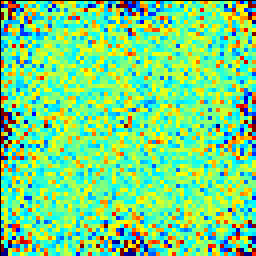
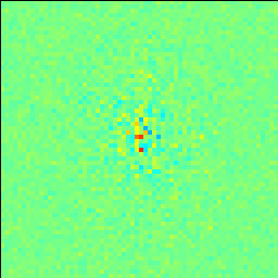
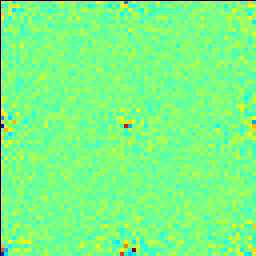
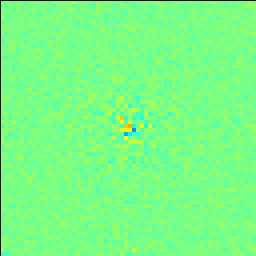
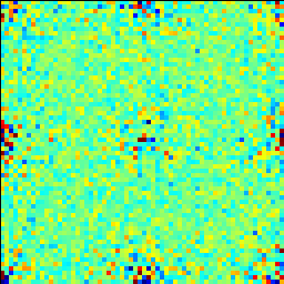
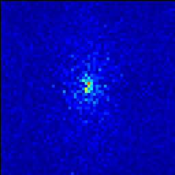
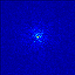
In Figure 1 we present selected static structure factors from the simulation. In each case, the color scale is adjusted to represent $\pm 20$% of the equilibrium value, which is independent of wave number. The simulations show excellent agreement with the theoretical values. The structure factor for $\rho$, given by $\langle(\delta\hat{\rho})(\delta\hat{\rho}^{*})\rangle$, is the noisiest. This occurs because the continuity equation, (6), does not contain either a diffusive term or a stochastic flux so density fluctuations are solely driven by velocity fluctuations in the hyperbolic flux. Nevertheless, the (unnormalized) variance of density (i.e., the average static structure factor over all wavenumbers) is $5.7904\times 10^{-11}~{}\mathrm{g}^{2}/\mathrm{cm}^{6}$, which is within 0.07% of the analytic value of $5.7942\times 10^{-11}~{}\mathrm{g}^{2}/\mathrm{cm}^{6}$. The other relatively noisy structure factor is $\langle(\delta\hat{\rho}_{4})(\delta\hat{\rho}_{4}^{*})\rangle$, which is a result of the relatively low mole fraction which makes $\rho_{4}$ noisy with over 40% instantaneous variation. Here again, the average variance is correct to within 0.15%. Note that the grid-based finite-volume methods we employ here are neither translationally (Gallilean) invariant nor rotationally invariant, and this leads to non-isotropic structure factors for finite time step sizes (i.e., to non-isotropic spatial truncation errors), particularly for high wave numbers.

(a) (b)

(c) (d)

(e) (f)

Figure 1: (Color online) Static structure factors. (a) $\langle(\delta\hat{\rho})(\delta\hat{\rho}^{*})\rangle)$, (b) $\langle(\delta\widehat{J_{x}})(\delta\widehat{J_{x}}^{*})\rangle$, (c) $\langle(\delta\widehat{\rho E})(\delta\widehat{\rho E}^{*})\rangle$, (d) $\langle(\delta\hat{\rho_{1}})(\delta\hat{\rho_{1}}^{*})\rangle$, (e) $\langle(\delta\hat{\rho_{4}})(\delta\hat{\rho_{4}}^{*})\rangle$, (f) $\langle(\delta\hat{T})(\delta\hat{T}^{*})\rangle$. Data range is set to $\pm 20\%$ of the theoretical value of unity, as shown in the color bar. The wave number domain represented here is $[-3.93\times 10^{7},3.93\times 10^{7}]\times[-3.93\times 10^{7},3.93\times 10^{7}]$ in units of cm^-1.

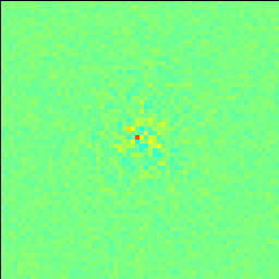
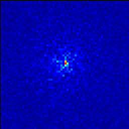
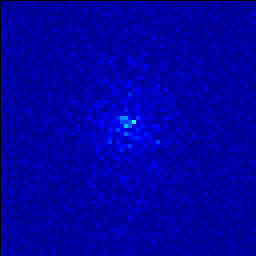
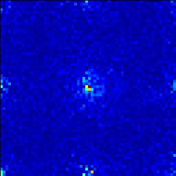
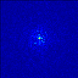
We also examine correlations between different hydrodynamic variables as a function of wave number. A set of representative correlations are presented in Figure 2. In each of these cases the correlation should be zero and the results show that the normalized values are indeed quite small. Of particular note is absence of a correlation for different components of momentum ($|\langle(\delta\widehat{J_{x}})(\delta\widehat{J_{y}}^{*})\rangle|\approx 0$) validating the treatment of the stress tensor in the momentum equations. Furthermore, the correlation between $\delta\rho_{1}$ and $\delta\rho_{4}$ is near zero, illustrating that there is no spurious correlation in the treatment of species diffusion. The relaxation time for the largest wavelengths is extremely long, which is manifested as a large statistical error at the lowest wavenumbers.

(a) (b)

(c) (d)

(e) (f)

Figure 2: (Color online) Magnitude of correlations: (a) $|\langle(\delta\hat{\rho})(\delta\widehat{J_{x}}^{*})\rangle|$, (b) $|\langle(\delta\hat{\rho})(\delta\hat{T}^{*})\rangle|$, (c) $|\langle(\delta\widehat{J_{x}})(\delta\widehat{J_{y}}^{*})\rangle|$, (d) $|\langle(\delta\widehat{J_{x}})(\delta\widehat{\rho E}^{*})\rangle|$, (e) $|\langle(\delta\hat{\rho_{1}})(\delta\hat{\rho}_{4}^{*})\rangle|$, (f) $|\langle(\delta\widehat{v_{x}})(\delta\hat{T}^{*})\rangle|$. In all cases the theoretical value is zero for all wave numbers. Data range is set to $20\%$ of the normalization, as shown in the color bar. The wave number domain represented here is $[-3.93\times 10^{7},3.93\times 10^{7}]\times[-3.93\times 10^{7},3.93\times 10^{7}]$ in units of cm^-1.

IV.2 Long-ranged Correlations in a Diffusion Barrier

The next example considers a non-equilibrium system in which the fluctuations exhibit long-range correlations in the presence of concentration gradients. Here we use a hard sphere gas mixture where the three gases (called Red, Blue, and Green or R, B, G) have equal molecular masses, taken as the mass of argon used in the previous example. Furthermore, Red and Blue are the same diameter, taken as that of argon, so that they are dynamically equivalent, with the diameter of Green being a factor of 10 larger. We set $Y_{R}=Y_{B}=0.25$ and $Y_{G}=0.5$ at the center of the domain and impose gradients of $dY_{R}/dy=28.935$, $dY_{B}/dy=90.760$ and $dY_{G}/dy=-119.695~{}\mathrm{cm}^{-1}$ for Red, Blue and Green, respectively across the domain. These conditions produce a “diffusion barrier” for the Red species, that is, the deterministic flux of Red is zero in spite of its gradient. The initial temperature in the domain is 300K and the initial pressure is one atmosphere. The top and bottom boundaries are no slip walls at a constant temperature of 300K with fixed reservoir boundaries for concentrations. Fluctuating hydrodynamics theory predicts that the spectrum of the concentration fluctuations exhibits long-range correlations due to the nonequilibrium conditions, even for the non-fluxing Red species, see derivation in Appendix B.

Obtaining good statistics requires a long simulation, consequently we use a domain that is only one cell thick in the $z$-direction, corresponding to an essentially two-dimensional domain. It can be shown using linearized fluctuating hydrodynamics (i.e., small fluctuations, which corresponds to a system of thickness much larger than molecular in the $z$-direction) that the spectrum of the concentration fluctuations is not affected by dimensionality. Namely, upon taking a Fourier transform in the directions perpendicular to the gradient, only the square of the perpendicular component of the wavevector enters, and in three dimensions one obtains the same spectrum as a function of the modulus of the wavevector as one does in two dimensions. This is easily seen in a quasi-periodic approximation, as detailed in Appendix B, but is true even in the presence of confinement GiantFluctFiniteEffects .

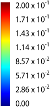
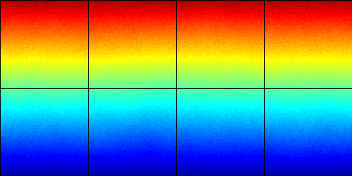
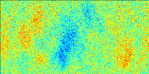
We take $\Delta x=\Delta y=\Delta z=2.7\times 10^{-5}$ cm on a $256\times 128\times 1$ domain and a time step of $\Delta t=10^{-10}$ s. A no slip boundary was used in the $y$ direction and periodic boundary conditions were used in the $x$ direction. The simulation is run for 200000 steps to relax to a statistical steady state and then run for an additional $2.8$ million steps, computing $\langle(\delta\hat{\rho}_{R})(\delta\hat{\rho}_{R})^{*}\rangle$, $\langle(\delta\hat{\rho}_{B})(\delta\hat{\rho}_{B})^{*}\rangle$ and $\langle(\delta\hat{\rho}_{R})(\delta\hat{\rho}_{B})^{*}\rangle$ in Fourier space on the vertically averaged profiles every 10 steps. An image illustrating a typical snapshot of $\rho_{R}$ is shown in Figure 3a. In Figure 3b we subtract off the background variation in $\rho_{R}$ to more clearly show the large scale structures. Horizontal variation of $\rho_{R}$ is apparent in the image.

a)

b)

Figure 3: (Color online) Typical snapshot of density of Red species in diffusion barrier simulation is shown in (a). In (b) we subtract the background stratification and show the variation from the background. The range of the color scale in (b) is approximately $\pm 5\sigma_{R}$ where $\sigma_{R}$ is the standard deviation of equilibrium fluctuations based on the value of $\rho_{R}$ in the center of the system. The domain is $6.912\times 10^{-3}$ cm $\times$ $3.456\times 10^{-3}$ cm $\times$ $2.7\times 10^{-5}$ cm. Units are g/cm³.

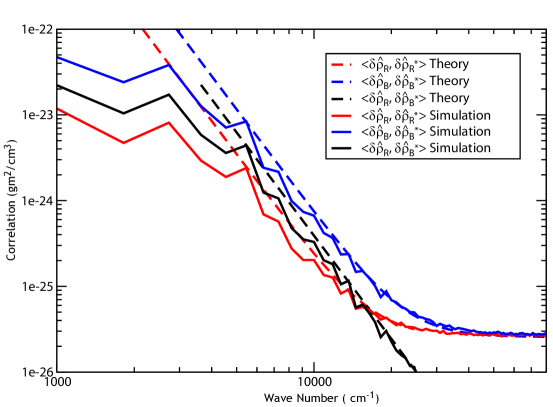
To provide a quantitative characterization of the large-scale fluctuations, we plot in Figure 4 a comparison of the computed static spectra of the species densities, averaged along the direction of the gradient, with theory (see Appendix B). It is these spectra that can be measured experimentally using low-angle light-scattering and shadowgraph techniques. We note that at low wave numbers the comparison breaks down because of finite size effects Zarate_07 . Otherwise the agreement between theory and simulation is excellent.

These results show that the correlations are long-ranged with the characteristic $k^{-4}$ power-law decay GiantFluctuations_Universal ; Vailati_11 ; SoretDiffusion_Croccolo , as in binary mixtures DiffusionRenormalization , even for the first species which has no mass flux. This demonstrates that the long-ranged correlations are associated with the system being out of thermodynamic equilibrium, and not with diffusive fluxes per se. Interestingly, we find that there are giant fluctuations in all species and also giant correlations between the fluctuations in different species. It is anticipated that measurement of these giant fluctuations in ternary mixtures can be used to calculate diffusion and Soret coefficients in mixtures SoretDiffusion_Croccolo . The main difficulty is the ability to experimentally observe the fluctuations in different species independently.

Figure 4: (Color online) Static structure factor of vertically-averaged densities showing effect of giant fluctuations. Dashed lines represent the predictions of linearized fluctuating hydrodynamics theory, see Appendix B. The constant limit obtained at high $k$ in the two autocorrelations corresponds to the equilibrium values given by Eq. 56.

IV.3 Diffusion-driven Rayleigh-Taylor Instability

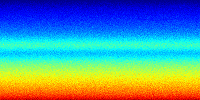
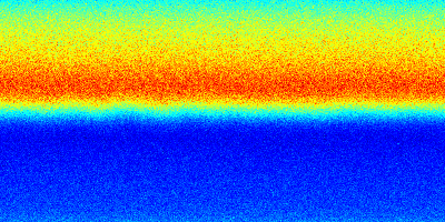
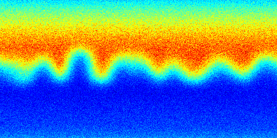
In this example, we illustrate how multicomponent diffusion can induce density stratification leading to a Rayleigh-Taylor instability BouyancyFluidsBook ; MultispeciesDiffusionInstability . We model a four species hard sphere mixture in which two of the species are light particles and two are heavy particles, specifically, $m_{1}=m_{3}<m_{2}=m_{4}$. For each mass, we have two different diameters, large and small, specifically, $d_{1}=d_{4}<d_{2}=d_{3}$; see Table 2. We initialize two layers, each of which has identical numbers of light and heavy particles in hydrostatic equilibrium with pressure of one atmosphere at the bottom of the domain. The result is a stably stratified isothermal initial condition of 300K with a switch in composition in the middle of the domain as shown in Table 2. The simulation used a $400\times 400\times 200$ grid with $\Delta x=\Delta y=\Delta z=6\times 10^{-6}$ cm and $\Delta t=5\times 10^{-12}$ s. Gravity is set to $g=4\times 10^{12}~{}\mathrm{cm/s}^{2}$ in order to reduce the time needed for the instability to develop. Boundary conditions are periodic in $x$ and $y$ with specular walls in the $z$ direction.

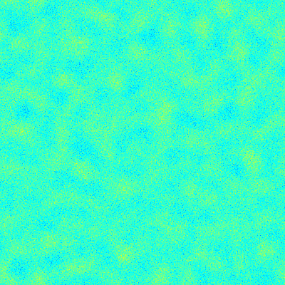
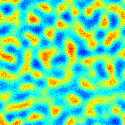
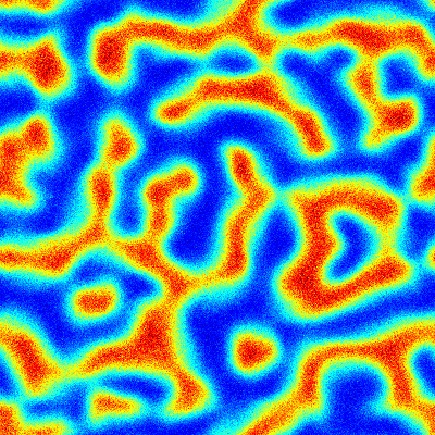
The large particles diffuse slowly compared with the small particles so that diffusion of the latter dominates the early dynamics. Initially the small, light particles are concentrated in the upper half of the domain while the small, heavy particles are concentrated on the lower half. This results in diffusion creating an unstable (heavier fluid on top of lighter fluid) density stratification MultispeciesDiffusionInstability , as shown in Figure 5. At later times fluctuations within the system trigger a Rayleigh-Taylor instability, as illustrated in Figures 6 and 7 which show the density of species 2 (large, heavy particles).

Species	Molecular Weight (g)	Diameter (cm)	$Y_{k}$ at top	$Y_{k}$ at bottom
Species 1	2.0	2.0 $\times 10^{-8}$	0.4	0.1
Species 2	20.0	20.0 $\times 10^{-8}$	0.4	0.1
Species 3	2.0	20.0 $\times 10^{-8}$	0.1	0.4
Species 4	20.0	2.0 $\times 10^{-8}$	0.1	0.4

Table 2: Molecular properties and configuration for the diffusion Rayleigh-Taylor instability.

Figure 5: (Color online) Vertical cross section of total density, $\rho$, for the Rayleigh-Taylor instability simulation at early times ($t=2.5\times 10^{-8}$ s). The cross secion shown is $2.4\times 10^{-3}$ cm $\times$ $1.2\times 10^{-3}$ cm. Units are g/cm³.

(a)      

(b)      

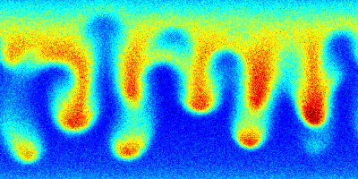
(c)       The cross secion shown is $2.4\times 10^{-3}$ cm $\times$ $1.2\times 10^{-3}$ cm. Units are g/cm³.

Figure 6: (Color online) Vertical cross section of $\rho_{2}$, the species with large, heavy particles. Frames correspond to (a) $t=7.5\times 10^{-8}$ s, (b) $t=15.0\times 10^{-8}$ s, and (c) $t=22.5\times 10^{-8}$ s.

(a) (b)

(c)      

Figure 7: (Color online) Horizontal slice through the center of the domain showing $\rho_{2}$ at (a) $t=7.5\times 10^{-8}$ s, (b) $t=15.0\times 10^{-8}$ s, and (c) $t=22.5\times 10^{-8}$ s. The cross secion shown is $2.4\times 10^{-3}$ cm $\times$ $2.4\times 10^{-3}$ cm. Units are g/cm³.

IV.4 Reverse Diffusion Experiment

Our final example illustrates an application of the methodology using realistic gas properties. In particular, we consider a three species mixture whose constituents are molecular hydrogen, carbon dioxide, and nitrogen. Instead of using the hard sphere model, for this final test case the fluid properties of the gas mixture were accurately modeled using EGLIB EGLIB , a general-purpose Fortran library for evaluating transport and thermodynamic properties of gas mixtures.

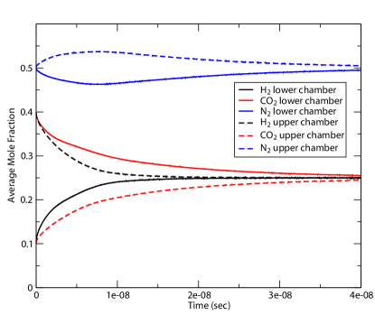
This test case is qualitatively similar to the reverse diffusion experiments of Duncan and Toor DuncanToor . The domain is split into two sections (chambers in the experiment) with equal pressures, temperatures, and nitrogen densities. The lower half of the domain is rich in carbon dioxide ($X_{H_{2}}=0.1$, $X_{CO_{2}}=0.4$, $X_{N_{2}}=0.5$) while the upper half is rich in hydrogen ($X_{H_{2}}=0.4$, $X_{CO_{2}}=0.1$, $X_{N_{2}}=0.5$). The system is initialized at $T=312.5$K and atmospheric pressure. The simulation is performed in a $32\times 32\times 64$ mesh so that each half is $32^{3}$ with a uniform mesh spacing of $2.7\times 10^{-6}$ cm in each direction with periodic boundaries in $x$ and $y$ and a specular walls in the $z$. The simulation is run for 100000 times steps with $\Delta t=4.\times 10^{-13}$ s. We note that there is no gravity in this problem and ordinary diffusion occurs for the carbon dioxide and hydrogen.

(a) (b) (c) (d) (e)

Figure 8: (Color online) Slices showing temporal evolution of $\rho_{N_{2}}$. Frames correspond to (a) $t=0.0$ s, (b) $t=4.0\times 10^{-9}$ s, (c) $t=8.0\times 10^{-9}$ s, (d) $t=24.0\times 10^{-9}$ s, and (e) $t=40.0\times 10^{-9}$ s. Cross section shown is $8.64\times 10^{-5}$ cm $\times$ $2.32\times 10^{-5}$ cm. Units are g/cm³.

In Figure 8, we show slices of nitrogen density, $\rho_{N_{2}}$, at a sequence of times. At $t=4.0\times 10^{-9}$ s we see that, although its concentration is initially uniform, due to interdiffusion effects there has been a flux of $N_{2}$ into the upper half of the domain. In spite of the adverse gradient, diffusive transport continues to increase the amount of $N_{2}$ in the upper half as seen in Figure 8c. This “reverse diffusion” of nitrogen is driven by the rapid diffusion of $H_{2}$ out of the upper half, as compared with the slow diffusion of carbon dioxide into it. The last two frames in Figure 8 show the slow return towards uniform nitrogen concentration.

This reverse diffusion phenomenon is shown quantitatively in Figure 9 where we plot the time history of the average mole fractions in the upper and lower halves of the domain. We see that there is a flux of $N_{2}$ into the upper half until approximately $t=8.0\times 10^{-9}$ s in spite of the adverse $N_{2}$ gradient, at which point a diffusion barrier occurs (gradient of $N_{2}$ without a flux). At later times the diffusion is “normal” for all three species. We note that the data in Figure 9 is in qualitative agreement with the experimental results of Duncan and Toor; the primary differences between the simulation and the experimental set-up are the size and geometry of the system. Thermal fluctuations do not play a significant role in this numerical experiment, although the appearance of giant fluctuations due to the transient concentration gradients is expected. The primary purpose of this final numerical test is to demonstrate the ability of our implementation to simulate gas mixtures using transport and thermodynamic properties given by the EGLIB library, allowing quantitative comparison with experiments.

Figure 9: (Color online) Time evolution of average composition in upper and lower halves of the domain.

V Conclusions and Future Work

The four examples in the previous section confirm the accuracy of our numerical formulation for the multispecies fluctuating Navier-Stokes equations. Furthermore, they illustrate some of the interesting phenomena unique to such fluid mixtures. While these numerical examples were all gas mixtures the methodology is directly extendable to liquids, the main challenge being the formulation of accurate thermodynamic and transport properties TernaryEquilibriumFluct . Work in this direction is currently underway and fluctuating hydrodynamics should prove useful for experimental studies of the properties of liquid mixtures SoretDiffusion_Croccolo .

A numerical limitation of the methodology presented here is that the stochastic PDE solver is explicit. This restricts practical application of the method to the study of phenomena of mesoscopic duration ($\approx$ microsecond) given the magnitude of the algorithm’s stable time step. This restriction is particularly severe for liquid mixtures for which there are orders of magnitude of separation between the fast acoustic, intermediate viscous, and slow diffusive time scales, at which phenomena of interest occur (e.g., minutes or hours for giant fluctuation experiments Vailati_11 ). To lift the time step limitation we are investigating low-Mach number approximations for mixtures DonevLowMach2013 . Another important avenue of research we are presently persuing is to extend our formulation to non-ideal multispecies mixtures of non-ideal fluids TernaryEquilibriumFluct ; NewIrrevThermoBook .

We are also extending the formulation to reacting, multi-component mixtures, which will lay the groundwork for the investigation of a wide variety phenomena combining hydrodynamic and chemical fluctuations. Numerical methods for fluctuating reaction-diffusion systems date back to the early 1970’s Gillespie1976403 ; NicolisPrigogine ; GardinerBook but these methods neglect all hydrodynamic transport other than diffusion and typically diffusion is also simplified GillespieReview2013 . While this is a good approximation for many phenomena, a complete description of transport is required for combustion.

Appendix A Variances in a Multicomponent Gas Mixture

For species $i$ the number of molecules in a volume $V$ is $N_{i}=V\rho_{i}/m_{i}$ where $m_{i}$ is the mass of a molecule. At equilibrium for an ideal gas this number is Poisson distributed and independent of other species so $\langle\delta N_{i}\delta N_{j}\rangle=\bar{N}_{i}\delta_{ij}$ and,

$$\langle\delta\rho_{i}\delta\rho_{j}\rangle_{eq}=\frac{\bar{\rho}_{i}^{2}}{\bar{N}_{i}}\delta_{ij}=\frac{\bar{\rho}_{i}^{2}k_{B}\bar{T}}{\bar{P}\bar{X}_{i}V}\delta_{ij},$$ (36)

where the subscript “eq” indicates an equilibrium result. At equilibrium the variance of density is thus,

$$\langle\delta\rho^{2}\rangle_{\mathrm{eq}}=\sum_{i}\sum_{j}\langle\delta\rho_{i}\delta\rho_{j}\rangle_{\mathrm{eq}}=\sum_{i}\frac{\bar{\rho}_{i}^{2}}{\bar{N}_{i}}=\frac{\bar{\rho}^{2}}{\bar{N}}\sum_{i}\frac{Y_{i}^{2}}{X_{i}}=\frac{\bar{\rho}^{2}k_{B}\bar{T}}{\bar{P}V}\sum_{i}\frac{Y_{i}^{2}}{X_{i}}.$$ (37)

From this,

$$\langle\delta\rho^{2}\rangle_{\mathrm{eq}}=\zeta\langle\delta\rho^{2}\rangle_{\mathrm{eq}}^{(1)}\qquad\mathrm{where}\qquad\zeta=\sum_{i}\frac{Y_{i}^{2}}{X_{i}}$$ (38)

and $\langle\delta\rho^{2}\rangle_{\mathrm{eq}}^{(1)}=\bar{\rho}^{2}/\bar{N}$ is the variance for a single species gas at the same density, temperature, and pressure (i.e., same $\bar{N}=\bar{P}V/k_{B}\bar{T}$). Note that all of the expressions in this appendix may be generalized easily to spatial correlations, for example,

$$\langle\delta\rho(\mathbf{r})\delta\rho(\mathbf{r}^{\prime})\rangle=\frac{\bar{\rho}^{2}k_{B}\bar{T}}{\bar{P}}\delta(\mathbf{r}-\mathbf{r}^{\prime})\sum_{i}\frac{Y_{i}^{2}}{X_{i}}.$$ (39)

For the variance and correlations of momentum the results are the same as those for a single species gas when $\bar{\mathbf{v}}=0$, specifically,

$$\langle\delta\rho\delta\mathbf{J}\rangle_{\mathrm{eq}} = 0$$ (40)

$$\langle\delta J_{\alpha}\delta J_{\beta}\rangle_{\mathrm{eq}} = \frac{\bar{\rho}k_{B}\bar{T}}{V}\delta_{\alpha\beta}.$$ (41)

Similarly, for velocity,

$$\langle\delta\rho\delta\mathbf{v}\rangle_{\mathrm{eq}} = 0$$ (42)

$$\langle\delta v_{\alpha}\delta v_{\beta}\rangle_{\mathrm{eq}} = \frac{k_{B}\bar{T}}{\bar{\rho}V}\delta_{\alpha\beta}.$$ (43)

Finally, for energy fluctuations,

$$\delta\mathcal{E}=\delta(\rho E) = \delta\left(\frac{1}{2}\rho v^{2}+\sum_{i}\rho_{i}e_{i}(T)\right)$$ (44)

$$= \bar{\rho}\bar{\mathbf{v}}\cdot\delta\mathbf{v}+\frac{1}{2}\bar{v}^{2}\delta\rho+\sum_{i}\delta\rho_{i}e_{i}(\bar{T})+\bar{\rho}c_{v}(\bar{T})\,\delta T,$$ (45)

where

$$c_{v}(T)=\frac{1}{\rho}\sum_{i}\rho_{i}c_{v,i}(T)=\sum_{i}Y_{i}c_{v,i}(T)$$ (46)

is the molar averaged specific heat. Note that if $c_{v}$ is independent of temperature then $e_{i}(\bar{T})=c_{v,i}\bar{T}$.

The resulting variance and correlations for energy are,

$$\langle\delta\rho\delta\mathcal{E}\rangle_{\mathrm{eq}} = \sum_{i}e_{i}(\bar{T})\langle\delta\rho_{i}^{2}\rangle_{\mathrm{eq}};$$ (47)

$$\langle\delta\mathbf{J}\delta\mathcal{E}\rangle_{\mathrm{eq}} = 0;$$ (48)

$$\langle\delta\mathcal{E}^{2}\rangle_{\mathrm{eq}} = \sum_{i}e_{i}(\bar{T})^{2}\langle\delta\rho_{i}^{2}\rangle_{\mathrm{eq}}+\bar{\rho}^{2}c_{v}(\bar{T})^{2}\langle\delta T^{2}\rangle_{\mathrm{eq}}.$$ (49)

Similarly for temperature,

$$\langle\delta\rho\delta T\rangle_{\mathrm{eq}} = 0;$$ (50)

$$\langle\delta\mathbf{v}\delta T\rangle_{\mathrm{eq}} = 0;$$ (51)

$$\langle\delta T^{2}\rangle_{\mathrm{eq}} = \frac{k_{B}T^{2}}{\bar{\rho}c_{v}(\bar{T})V}.$$ (52)

Appendix B Giant fluctuations in a ternary mixture

This appendix outlines the fluctuating hydrodynamics theory for the long-range correlations of concentration fluctuations in a ternary mixture, in order to model the simulations described in Section IV.2. We neglect the Dufour effect and assume the system to be isothermal, taking contributions from temperature fluctuations to be of higher order. Furthermore, we neglect gravity, assume the system is incompressible, and take the density and transport coefficients to be constant. We consider a “bulk” system Zarate_07 , i.e., we neglect the influence of the boundaries. This gives an accurate approximation for wavenumbers that are large compared to the inverse height of the domain; for smaller wavenumbers the boundaries are expected to suppress the giant fluctuations Zarate_07 ; GiantFluctFiniteEffects ; Vailati_11 . Lastly, we initially ignore the equilibrium fluctuations in the calculation and simply add them to the non-equilibrium contribution at the end. This is not necessary and the additional stochastic diffusive fluxes can easily be accounted for at the expense of algebraic complications. This confirms that the equilibrium fluctuations enter additively to the nonequilibrium ones calculated here, as confirmed by an anonymous reviewer.

As in the problem considered in Section IV.2, we assume all of the concentration gradients are in the same direction (say, the $y$ axis). The incompressibility constraint is most easily handled by applying a $\bm{\nabla}\times\bm{\nabla}\times$ operator to the momentum equation to obtain a system involving only the component of the velocity parallel to the gradient (in this case, the $y$-direction). Zarate_07 With the above, the momentum and concentration equations yield,

$$\partial_{t}\left(\bm{\nabla}^{2}v_{\parallel}\right) = \nu\bm{\nabla}^{2}\left(\bm{\nabla}^{2}v_{\parallel}\right)+\rho_{0}^{-1}\bm{\nabla}\times\bm{\nabla}\times\left(\bm{\nabla}\cdot\widetilde{\bm{\Pi}}\right)$$

$$\partial_{t}\left(\delta\mathbf{Y}\right) = -v_{\parallel}\bm{f}+\bm{{D}}\bm{\nabla}^{2}\left(\delta\mathbf{Y}\right),$$

where $\rho_{0}$ is the constant density, and $\nu=\eta/\rho_{0}$ is the kinematic viscosity. Here $\bm{{D}}=\rho^{-1}\bm{C}\left(\frac{\partial\bm{X}}{\partial\bm{Y}}\right)$ is a matrix of diffusion coefficients and $\partial\bm{X}/\partial\bm{Y}$ is the Jacobian of the transformation from mass to mole fractions, which is a function of the mean molecular mass and the individual species molecular masses. Here $\bm{f}=d\langle{\mathbf{Y}}\rangle/dy$ are the imposed mass fraction gradients and $\delta\mathbf{Y}=\mathbf{Y}-\langle{\mathbf{Y}}\rangle$ is the concentration fluctuation.

This system of equations can be most easily solved in the Fourier domain, where it becomes

$$\partial_{t}\hat{v}_{\parallel} = -\nu k^{2}\hat{v}_{\parallel}+\hat{F}$$ (53)

$$\partial_{t}\left(\delta\hat{\mathbf{Y}}\right) = -\hat{v}_{\parallel}\bm{f}-k^{2}\bm{{D}}\delta\hat{\mathbf{Y}},$$ (54)

and the covariance of the random forcing $\hat{F}$ is (see (5.12) in Ref. Zarate_07 )

$$\left\langle\hat{F}\hat{F}^{\star}\right\rangle=\frac{2k_{B}T_{0}}{\rho_{0}}\nu k_{\perp}^{2},$$

where $\bm{k}_{\perp}$ is the component of the wavevector in the plane perpendicular to the gradient and $T_{0}$ is the constant temperature. The equilibrium covariance of the fluctuations, written as a matrix of static structure factors,

$$\bm{S}=\left[\begin{array}[]{cc}\left\langle\hat{v}_{\parallel}\hat{v}_{\parallel}^{\star}\right\rangle&\left\langle\left(\delta\hat{\mathbf{Y}}\right)\hat{v}_{\parallel}^{\star}\right\rangle\\ \left\langle\hat{v}_{\parallel}\left(\delta\hat{\mathbf{Y}}\right)^{\star}\right\rangle&\left\langle\left(\delta\hat{\mathbf{Y}}\right)\left(\delta\hat{\mathbf{Y}}\right)^{\star}\right\rangle\end{array}\right]$$

can be obtained most directly by writing the equations (53,54) in the form of an Ornstein-Uhlenbeck (OU) process,

$$\partial_{t}\left[\begin{array}[]{c}\hat{v}_{\parallel}\\ \delta\hat{\mathbf{Y}}\end{array}\right]=\left[\begin{array}[]{cc}-\nu k^{2}&0\\ -\bm{f}&-k^{2}\bm{{D}}\end{array}\right]\left[\begin{array}[]{c}\hat{v}_{\parallel}\\ \delta\hat{\mathbf{Y}}\end{array}\right]+\left[\begin{array}[]{c}\hat{F}\\ \bm{0}\end{array}\right]=\bm{M}\left[\begin{array}[]{c}\hat{v}_{\parallel}\\ \delta\hat{\mathbf{Y}}\end{array}\right]+\bm{m},$$

and using the well-known equation for the equilibrium covariance of an OU process GardinerBook (see, for example, derivation in Ref. Donev_10 ),

$$\bm{M}\bm{S}+\bm{S}\bm{M}^{\star}=-\left\langle\bm{m}\bm{m}^{\star}\right\rangle.$$ (55)

This is a linear system of equations for the static structure factors that can easily be solved using computer algebra systems. Note that here the equation for the third species is redundant and it is simpler to develop the theory by considering the equations for only the first two species.

Turning now to the specific example of a ternary mixture considered in Section IV.2: The molecular masses are identical and therefore mole and mass fractions are the same, $\partial\bm{X}/\partial\mathbf{Y}=\bm{I}$. Furthermore, the first two of the three species are indistinguishable so $\bm{{D}}$ has the simple form,

$$\bm{{D}}=\left[\begin{array}[]{cc}{D}_{1}&{D}_{2}\\ {D}_{2}&{D}_{1}\end{array}\right].$$

The system is set up with a diffusion barrier, that is, there is no deterministic flux for the first species. This implies that,

$$f_{1}=\frac{d\langle{Y}_{1}\rangle}{dy}=-\frac{{D}_{2}}{{D}_{1}}\frac{d\langle{Y}_{2}\rangle}{dy}.$$

We consider the spectrum of the fluctuations of the partial densities averaged along the direction of the gradient, as is measured in experiments Vailati_11 ; GiantFluctuations_Universal ; SoretDiffusion_Croccolo , i.e., we take $k_{\parallel}=0$, $\bm{k}=\bm{k}_{\perp}$. The solution of (55) gives the non-equilibrium contribution to the static structure factor for vertically-averaged concentration fluctuations to be

$$\left\langle\left(\delta\hat{\mathbf{Y}}\right)\left(\delta\hat{\mathbf{Y}}\right)^{\star}\right\rangle_{\text{neq}}=K\left[\begin{array}[]{cc}{\frac{8\,{{D}_{{1}}}^{3}+5\,{{D}_{{1}}}^{2}\nu-\nu\,{{D}_{{2}}}^{2}}{{{D}_{{1}}}^{2}{D}_{{2}}}}&-{\frac{3\,{{D}_{{1}}}^{2}\nu+\nu\,{{D}_{{2}}}^{2}+4\,{{D}_{{1}}}^{3}+4\,{{D}_{{2}}}^{2}{D}_{{1}}}{{{D}_{{2}}}^{2}{D}_{{1}}}}\\ \vskip 6.0pt plus 2.0pt minus 2.0pt\cr-{\frac{3\,{{D}_{{1}}}^{2}\nu+\nu\,{{D}_{{2}}}^{2}+4\,{{D}_{{1}}}^{3}+4\,{{D}_{{2}}}^{2}{D}_{{1}}}{{{D}_{{2}}}^{2}{D}_{{1}}}}&{\frac{{{D}_{{2}}}^{4}\nu+2\,{{D}_{{1}}}^{4}\nu+2\,{{D}_{{1}}}^{5}+{{D}_{{1}}}^{2}\nu\,{{D}_{{2}}}^{2}+2\,{{D}_{{2}}}^{4}{D}_{{1}}+4\,{{D}_{{1}}}^{3}{{D}_{{2}}}^{2}}{{{D}_{{1}}}^{2}{{D}_{{2}}}^{3}}}\end{array}\right]$$

where the common pre-factor is

$$K={\frac{{\it k_{B}T}}{2\rho\,{k}^{4}}}\cdot\frac{{D}_{{1}}{D}_{{2}}}{\left({D}_{{1}}-{D}_{{2}}\right)\left({D}_{{1}}+{D}_{{2}}\right)\left({D}_{{1}}+\nu+{D}_{{2}}\right)\left({D}_{{1}}+\nu-{D}_{{2}}\right)}\cdot f_{1}^{2}.$$

The equilibrium static structure factor for the mixture of ideal gases considered here is

$$\left\langle\left(\delta\hat{\mathbf{Y}}\right)\left(\delta\hat{\mathbf{Y}}\right)^{\star}\right\rangle_{\text{eq}}=\rho_{0}^{-2}\left[\begin{array}[]{cc}m_{1}\langle{\rho}_{1}\rangle&0\\ 0&m_{2}\langle{\rho}_{2}\rangle\end{array}\right]\;\;,$$ (56)

which is to be added to the nonequilibrium contribution to obtain the full spectrum, as shown in Fig. 4.

In the case of liquids, the Schmidt number is very large and ${D}_{1}\ll\nu$ and ${D}_{2}\ll\nu$ and the expressions simplify considerably,

$$\left\langle\left(\delta\hat{\mathbf{Y}}\right)\left(\delta\hat{\mathbf{Y}}\right)^{\star}\right\rangle_{\text{neq}}={\frac{{D}_{{1}}{D}_{{2}}{\it k_{B}T{|\nabla_{z}Y_{1}|}^{2}}}{2\eta\,{k}^{4}\left({D}_{{1}}-{D}_{{2}}\right)\left({D}_{{1}}+{D}_{{2}}\right)}}\left[\begin{array}[]{cc}{\frac{5\,{{D}_{{1}}}^{2}-{{D}_{{2}}}^{2}}{{{D}_{{1}}}^{2}{D}_{{2}}}}&-{\frac{3\,{{D}_{{1}}}^{2}+{{D}_{{2}}}^{2}}{{{D}_{{2}}}^{2}{D}_{{1}}}}\\ \vskip 6.0pt plus 2.0pt minus 2.0pt\cr-{\frac{3\,{{D}_{{1}}}^{2}+{{D}_{{2}}}^{2}}{{{D}_{{2}}}^{2}{D}_{{1}}}}&{\frac{{{D}_{{2}}}^{4}+2\,{{D}_{{1}}}^{4}+{{D}_{{1}}}^{2}{{D}_{{2}}}^{2}}{{{D}_{{1}}}^{2}{{D}_{{2}}}^{3}}}\end{array}\right].$$

This can be more straightforwardly obtained by simply deleting the inertial term $\partial_{t}\hat{v}_{\parallel}$ on the left-hand side of the momentum equation (53) GiantFluctFiniteEffects . Note however that the Schmidt number is not large for gas mixtures and one must retain the complete expression to obtain a good match to the numerical results.

References

- (1) A. Donev, J. B. Bell, A. de la Fuente, and A. L. Garcia, Phys. Rev. Lett. 106, 204501 (2011)
- (2) A. Donev, J. B. Bell, A. de la Fuente, and A. L. Garcia, Journal of Statistical Mechanics: Theory and Experiment 2011, P06014 (2011), http://stacks.iop.org/1742-5468/2011/i=06/a=P06014
- (3) K. Kadau, T. C. Germann, N. G. Hadjiconstantinou, P. S. Lomdahl, G. Dimonte, B. L. Holian, and B. J. Alder, Proc. Natl. Acad. Sci. 101, 5851 (2004)
- (4) K. Kadau, C. Rosenblatt, J. L. Barber, T. C. Germann, Z. Huang, P. Carles, and B. J. Alder, Proc. Natl. Acad. Sci. 104, 7741 (2007)
- (5) M. Moseler and U. Landman, Science 289, 1165 (2000)
- (6) J. Eggers, Phys. Rev. Lett. 89, 084502 (2002)
- (7) J. K. Sigurdsson, F. L. Brown, and P. J. Atzberger, Journal of Computational Physics 252, 65 (2013), ISSN 0021-9991, http://www.sciencedirect.com/science/article/pii/S0021999113004403
- (8) Y. Wang, J. K. Sigurdsson, E. Brandt, and P. J. Atzberger, Phys. Rev. E 88, 023301 (Aug 2013), http://link.aps.org/doi/10.1103/PhysRevE.88.023301
- (9) B. Nowakowski and A. Lemarchand, Phys. Rev. E 68, 031105 (2003)
- (10) A. Lemarchand and B. Nowakowski, Mol. Simul. 30, 773 (2004)
- (11) A. Vailati and M. Giglio, Nature 390, 262 (1997)
- (12) A. Vailati and M. Giglio, Phys. Rev. E 58, 4361 (1998)
- (13) A. Vailati, R. Cerbino, S. Mazzoni, C. J. Takacs, D. S. Cannell, and M. Giglio, Nature Communications 2, 290 (2011)
- (14) J. M. Yuk, J. Park, P. Ercius, K. Kim, D. J. Hellebusch, M. F. Crommie, J. Y. Lee, A. Zettl, and A. P. Alivisatos, Science 336, 61 (2012)
- (15) J. M. O. de Zarate and J. V. Sengers, Hydrodynamic Fluctuations in Fluids and Fluid Mixtures (Elsevier Science, 2007)
- (16) L. D. Landau and E. M. Lifshitz, Fluid Mechanics, Course of Theoretical Physics, Vol. 6 (Pergamon Press, 1959)
- (17) R. F. Fox and G. E. Uhlenbeck, The Phys. of Fluids 13, 1893 (1970)
- (18) R. F. Fox and G. E. Uhlenbeck, The Phys. of Fluids 13, 2881 (1970)
- (19) A. Ikoma, T. Arima, S. Taniguchi, N. Zhao, and M. Sugiyama, Physics Letters A 375, 2601 (2011), ISSN 0375-9601, http://www.sciencedirect.com/science/article/pii/S0375960111006669
- (20) J. P. Mithen, J. Daligault, and G. Gregori, Phys. Rev. E 83, 015401 (Jan 2011), http://link.aps.org/doi/10.1103/PhysRevE.83.015401
- (21) C. Cohen, J. W. H. Sutherland, and J. M. Deutch, Phys. and Chem. of Liquids 2, 213 (1971)
- (22) B. Law and J. Nieuwoudt, Phys. Rev. A 40, 3880 (1989)
- (23) J. Nieuwoudt and B. Law, Phys. Rev. A 42, 2003 (1989)
- (24) H. C. Ottinger, The J. Chem. Phys. 130, 114904 (2009)
- (25) J. M. Ortiz de Zárate, J. L. Hita, and J. V. Sengers, Comptes Rendus Mécanique(2013)
- (26) A. L. Garcia, M. M. Mansour, G. C. Lie, and E. Clementi, J. Stat. Phys. 47, 209 (1987)
- (27) M. M. Mansour, A. L. Garcia, G. C. Lie, and E. Clementi, Phys. Rev. Lett. 58, 874 (1987)
- (28) J. B. Bell, A. L. Garcia, and S. A. Williams, Phys. Rev. E 76, 016708 (2007)
- (29) J. B. Bell, A. L. Garcia, and S. A. Williams, ESAIM: Mathematical Modelling and Numerical Analysis 44, 1085 (2010)
- (30) A. Donev, E. Vanden-Eijnden, A. L. Garcia, and J. B. Bell, Comm. Appl. Math and Comp. Sci. 5, 149 (2010)
- (31) F. Balboa Usabiaga, J. Bell, R. Delgado-Buscalioni, A. Donev, T. Fai, B. Griffith, and C. Peskin, Multiscale Modeling & Simulation 10, 1369 (2012)
- (32) J. B. Duncan and H. L. Toor, AIChE Journal 8, 38 (1962)
- (33) S. R. DeGroot and P. Mazur, Non-Equilibrium Thermodynamics (North-Holland Publishing Company, Amsterdam, 1963)
- (34) R. Bird, W. Stewart, and E. Lightfoot, Transport Phenomena (John Wiley and Sons, 2006)
- (35) G. D. C. Kuiken, Thermodynamics of Irreversible Processes: Applications to Diffusion and Rheology (Wiley, 1994)
- (36) A. Ern and V. Giovangigli, EGLIB: A general-purpose Fortran library for multicomponent transport property evaluation, Version 3.4 (2004)
- (37) V. Giovangigli, Multicomponent Flow Modeling (Birkhauser Boston, 1999)
- (38) P. Espanol, Physica A: Statistical Mechanics and its Applications 248, 77 (1998), ISSN 0378-4371, http://www.sciencedirect.com/science/article/pii/S0378437197004615
- (39) This contribution is also zero if the external specific force acting on each species is constant, as with a constant gravitational acceleration.
- (40) S. Delong, B. E. Griffith, E. Vanden-Eijnden, and A. Donev, Phys. Rev. E 87, 033302 (Mar 2013), http://link.aps.org/doi/10.1103/PhysRevE.87.033302
- (41) We note that technically, we to not need to solve a separate continuity equation since . We do so here simply for diagnostic purposes.
- (42) P. Colella and P. R. Woodward, J. Comput. Phys. 54, 174 (1984)
- (43) A. Donev, A. J. Nonaka, Y. Sun, T. Fai, A. L. Garcia, and J. B. Bell, submitted to Comm. Appl. Math and Comp. Sci.(2013)
- (44) J. O. Hirschfelder, C. F. Curtiss, and R. B. Bird, Molecular Theory of Gases and Liquids (John Wiley and Sons, INC., New York, 1954)
- (45) V. D. Valk, Physica 29, 417 (1963)
- (46) J. M. Ortiz de Zárate, J. A. Fornés, and J. V. Sengers, Phys. Rev. E 74, 046305 (Oct 2006), http://link.aps.org/doi/10.1103/PhysRevE.74.046305
- (47) D. Brogioli, A. Vailati, and M. Giglio, Phys. Rev. E 61, R1 (Jan 2000), http://link.aps.org/doi/10.1103/PhysRevE.61.R1
- (48) F. Croccolo, H. Bataller, and F. Scheffold, The Journal of Chemical Physics 137, 234202 (2012), http://link.aip.org/link/?JCP/137/234202/1
- (49) J. Turner, Buoyancy Effects in Fluids (Cambridge Univ. Press, 1979)
- (50) P. M. J. Trevelyan, C. Almarcha, and A. D. Wit, Journal of Fluid Mechanics 670, 38 (2011)
- (51) D. T. Gillespie, Journal of Computational Physics 22, 403 (1976), ISSN 0021-9991, http://www.sciencedirect.com/science/article/pii/0021999176900413
- (52) G. Nicolis and I. Prigogine, Self-Organization in Non-Equilibrium Systems (Wiley, 1977)
- (53) C. Gardiner, Handbook of stochastic methods: for physics, chemistry, and the natural sciences, 4th ed. (Springer, 2009)
- (54) D. Gillespie, A. Hellander, and L. Petzold, J. Chem. Phys. 138 (2013)