Decentralized Signal Control for Urban Road Networks

Abstract

We propose in this paper a decentralized traffic signal control policy for urban road networks. Our policy is an adaptation of a so-called BackPressure scheme which has been widely recognized in data network as an optimal throughput control policy. We have formally proved that our proposed BackPressure scheme, with fixed cycle time and cyclic phases, stabilizes the network for any feasible traffic demands. Simulation has been conducted to compare our BackPressure policy against other existing distributed control policies in various traffic and network scenarios. Numerical results suggest that the proposed policy can surpass other policies both in terms of network throughput and congestion.

1 Introduction

Traffic congestion is a major problem in modern societies due to increasing population and economic activity. This motivates the need for better utilizing the existing infrastructures and for efficiently controlling the traffic flow in order to minimize the impact of congestion.

One of the key tools for influencing the efficiency of traffic flow in urban networks is traffic signal control that enables conflicting traffic to flow through intersections via the timing of green/red light cycles. It has long been recognized that the challenge is to find optimal cycle timing over many intersections so as to reduce the overall congestion and to increase the throughput through the network.

There has been much work in the past both on designing and optimizing isolated or coordinated signals that reactively resolve congestion in the urban networks. Broadly, there are two types of control that have been used for signal control: static and vehicle-actuated controls; see [10]. Static control (sometimes called “fixed time plan”) involves the optimization of the cycle time, the offset between nearby intersections, and the split of green times in different directions within a cycle. This can be optimized in isolation or in a coordinated manner, for instance to create a so-called green wave where vehicles always arrive at intersections during the green cycle time, e.g. [34, 8, 9, 14]. In contrast, vehicle-actuated controls use online measurements from on-road detectors (e.g., inductive loops) to optimize signal timings on a cycle-to-cycle basis in real time. Some examples of commonly used implementations are: SCOOT [12]; UTOPIA [20]; and the hierarchical scheme RHODES [23]. Combinations of both the fixed time plan and vehicle-actuated control also exist; one widely used example is SCATS [18].

Given a choice of the control scheme, various approaches to optimize the signal plans have been proposed. Examples include Mixed-Integer Linear Programming problems, see [8, 9, 6]; Linear Complementary Problem, see [5]; rolling horizon optimization using dynamic programming, see [7, 11, 23], or its combination with online learning algorithms , see [3]; store-and-forward models based on Model Predictive Control (MPC) optimization [13, 1, 31, 32, 30, 17], or MPC optimization with non-linear prediction [24]. Many of these approaches formulate the problem in a way that is centralized and thus are inherently not scalable. While the state of the art is the use of centralized techniques, improved scalability may be obtained using decentralized approaches. In this paper, we focus exclusively on decentralized schemes. Although such schemes are in their infancy, this research is one step along the path of improving such schemes to offer performance comparable with centralized schemes while retaining their scalability.

A scalable distributed approach is to solve a set of loosely coupled optimizations, one for each intersection, with coupling provided by traffic conditions. Two natural approaches are to control the traffic lights based on either (a) the expected number of vehicles to enter the intersection during the next cycle, or (b) the difference in traffic load on the road leading into the intersection and those leading out. These approaches are now deployable in practice thanks to emerging technologies, such as cameras and wireless communication enabling better access to real-time traffic data.

Notable among the first class is the work of [26], a so-called $P_{0}$ policy and its variants [4, 27], followed by the work of Lämmer and Helbing [15] where the switching cost between phases is taken into account. In this approach, each intersection estimates the amount of traffic that will arrive during the next complete cycle, and sets the split time such that each phase gets a time proportional to the number of cars expected to arrive on roads which have a green light during that phase. The lack of central control raises the possibility that intersections may interact in unexpected ways to cause instability. To limit this, a stabilization mechanism was proposed in [16]. However, beyond heuristic arguments, there remains no formal proof of stability of this approach.

Approach (b) including work by [33], [35] and [36] was inspired by research developed for packet scheduling in wireless networks: a so-called max weight or back pressure (refer to as BackPressure in this paper) algorithm [29, 21]. Like approach (a), BackPressure does not require any a priori knowledge of the traffic demand, but it has the added benefit of provable stability. To make that more precise, define a traffic load to a network as “feasible” if there exist splits at each intersection such that the queues do not build up indefinitely. Under certain simplifying assumptions, it can be shown that the queues under BackPressure do not build up indefinitely for any feasible traffic load. This will be made more formal in Section 3. In wireless networks, BackPressure can be computationally prohibitive, but in road networks [35, 33, 36], it admits a simple distributed implementation, just like approach (a).

It is worth noting that all the above mentioned policies [26, 27, 15, 33, 35, 36] make decisions periodically bases on the evaluations of traffic over a fixed time interval. These are called fixed cycle policies. For example, the BackPressure policy [35] determines the phase to be activated at the beginning of each fixed time slot, while the policy [16] decides whether to keep serving the current flow or switch to other flow at a regular time interval which can be arbitrary small.

Given the possibility of a stability guarantee by the BackPressure scheme, our objective in this work is to fully adapt it to the traffic control scenarios. To this end, we propose in this paper a new signal control strategy that addresses two weaknesses in the prior application of BackPressure to road networks [35, 33, 36] while retain and prove the important stability property of the BackPressure-based algorithms.

The first weakness to be addressed is that phases can form an erratic, unpredictable order in the previously proposed BackPressure policy. This is acceptable in the context of communications systems but for urban road traffic this is undesirable since erratic ordering of phases brings frustration to drivers and potentially causes confusion leading to dangerous actions. Moveover, if one inbound road is particularly backlogged, then it is possible that other roads are “starved” by being assigned a red light for an extended period. To rectify this, we modify BackPressure to a “cyclic phase” policy where a policy is said to be cyclic phase policy if it allocates strictly positive service time to all phases in each control decision, and thus, it is possible to arrange the phases into a fixed ordered sequence.

The second weakness that we address is that prior applications have required each intersection to know the “turning fractions”, that is, the fraction of traffic from each inbound road that will turn into each possible outbound road. We prove that the stability results still apply when these turning fractions are estimated using even very simple measurements; specifically, any unbiased estimator of the turning fractions suffices. Such stability proofs apply for a general network model but under idealized assumptions. Nonetheless these form an important step towards the application of BackPressure to real networks.

To test the practicality of the theoretical refinements described above, we also present the numerical comparison of the proposed BackPressure algorithm with the approach of [26] or [15, 16] without switching cost. The results suggest that our cyclic phase BackPressure policy tends to outperform other distributed polices both in terms of throughput and congestion. Although the performance of each policy varies widely depending on the parameter setting such as cycle length or decision frequency, under the optimal setting, the BackPressure with cyclic phase and without cyclic phase have better throughput in compare with the other policies.

The rest of this paper is organized as follows. We first present the notations and queue dynamics model before describing our proposed cyclic phase BackPressure policy in Section 2. The main results for stability of our policy are then provided in Section 3. These results in a certain sense mean, that we can interpret our policy as stabilizing the system for the largest possible set of arrival rates leading to sufficient throughput even in congested network. For readability, however, most of the mathematical details and derivations are listed in the Appendices of the paper. Section 4 presents the simulation results and numerical comparison of our scheme with other existing policies where we demonstrate the benefits of the proposed cyclic phase BackPressure signal control strategy. Finally, Section 5 concludes the paper and discusses future work.

2 Cyclic Phase BackPressure Traffic Signal Control

2.1 Notation and Network description

Consider a network of traffic intersections. This road network consists of a number of junctions, indexed by ${\mathcal{J}}$. Each junction $j\in{\mathcal{J}}$ consists of a number of in-roads, ${\mathcal{I}}_{j}$. Note that the ${\mathcal{I}}_{j}$ are mutually disjoint, and denote ${\mathcal{I}}=\cup_{j\in{\mathcal{J}}}{\mathcal{I}}_{j}$. A road with multiple lanes having different turning options (such as a left-turn only lane) is modeled as multiple in-roads, thus an in-road may model one or more lanes of traffic flow. Whether these traffic flows are conflicting or not is not considered in this setting. We use the inclusion $i\in j$ to indicate that in-road $i$ is part of junction $j$, and we let $j(i)$ notate the junction used by in-road $i$.

Each junction may serve different combinations of in-roads simultaneously. We call a combination of in-roads served simultaneously a service phase. A service phase for junction $j$ is represented by a vector $\sigma=(\sigma_{i}:i\in j)$ where $\sigma_{i}$ denotes the rate at which cars can be served from in-road $i$ at junction $j$ during phase $\sigma$. In particular, $\sigma_{i}>0$ if in-road $i$ has a green light during phase $\sigma$, or $\sigma_{i}=0$ otherwise.

Let ${\mathcal{S}}_{j}$ denote the set of phases at junction $j$. We will let ${\mathcal{L}}$ denote the set of links of the road traffic network. Each link represents a road connecting the junctions of the urban road network. Here we write $ii^{\prime}\in{\mathcal{L}}$ if it is possible for cars served at in-road $i$ junction $j$ to next join in-road $i^{\prime}$ junction $j^{\prime}$.

In the rest of this section we impose the additional constraint that all junctions have a common cycle length $T$, the time devoted to serving cars from the different in-roads at the junction. Thus we can model time as discrete and consider a slotted time model where $t=0,1,2,...$ denotes the number of the cycle about to be initiated. Control decisions in our policy are then made at the beginning of each time slot (so it is a fixed cycle policy which is similar to the policies in [16, 33, 26]). We also assume that all junctions have the same loss of service $L$ due to idle times during switches and setups. Thus at each time step, the system decides at each junction $j$ how much time within the next interval to spend serving each phase $\sigma\in{\mathcal{S}}_{j}$ with the constraint that each service phase must be enacted for some non-zero length of time and that the sum of the allocated times must not be greater than $T-L$. We assume that a car served at one junction in one time interval presents at an in-road of the next junction in its route at the next time interval.

2.2 Queue Dynamics Model

Let the queue length $Q_{i}(t)$ denote the number of cars at in-road $i\in{\mathcal{I}}$ at the beginning of the $t$th traffic cycle, and denote the vector of queue lengths by $Q(t)=(Q_{i}(t):{i\in{\mathcal{I}}})$. The decisions in the policy will be based on the measured queue lengths $\hat{Q}(t)$, which might differ from the actual value of $Q(t)$ by an error term as described in the following equation. $$\hat{Q}_{i}(t)=Q_{i}(t)+\delta_{i}(t),$$ (1) where the error term $\delta_{i}(t)$ is bounded and independent of $Q_{i}(t)$ or the terms at other in-roads. We denote the vector of the error terms by $\delta(t)=(\delta_{i}(t):{i\in{\mathcal{I}}})$.

Let $P^{j}_{\sigma}(t)$ denote the proportion of the traffic cycle at junction $j$ which is devoted to service phase $\sigma$. For any policy and for all $j\in{\mathcal{J}}$, we require $$\sum_{\sigma\in{\mathcal{S}}_{j}}P^{j}_{\sigma}(t)=1-\frac{L}{T}\qquad\text{and}\qquad P^{j}_{\sigma}(t)>0.$$ (2) Recall that $\sigma_{i}$ gives the rate at which cars can be served at in-road $i$ if the entire traffic cycle were devoted to phase $\sigma$, and $P^{j}_{\sigma}(t)$ gives the proportion of the traffic cycle devoted to service phase $\sigma$. Their product, $\sigma_{i}P^{j}_{\sigma}(t)$ gives the expected number of cars to leave in-road $i$ under service phase $\sigma$, provided the in-road is not emptied. Accordingly if we let the random variable $S_{i}(t)$ be the potential number of cars served from in-road $i$ at junction $j$ in traffic cycle $t$, the mean of $S_{i}(t)$ must satisfy

$${\mathbb{E}}[S_{i}(t)|Q(t),\delta(t)]=\sum_{\sigma\in{\mathcal{S}}_{j}}\sigma_{i}P^{j}_{\sigma}(t),$$ (3)

where we note that the proportions $P^{j}_{\sigma}(t)$ are allocated according to the decision in the policy based on $\hat{Q}(t)$, thus the dependency on $\delta(t)$. The random variable $S_{i}(t)$ only gives the number of cars served if the junction does not empty. Thus, it may be possible for $S_{i}(t)$ to be greater than the queue size $Q_{i}(t)$. In this case, $Q_{i}(t)$ will be the number of cars served. In other words, the number of cars actually served at junction $i$ is

$$S_{i}(t)\wedge Q_{i}(t)$$ (4)

where $x\wedge y=\min\{x,y\}$.

Further, when traffic is served it will move to neighbouring junctions. For $ii^{\prime}\in{\mathcal{L}}$, we let $p_{ii^{\prime}}(t)$ denote the proportion of cars served at in-road $i$ that subsequently join in-road $i^{\prime}$ at time $t$. We assume that cars within an in-road are homogeneous in the sense that each car at the junction has the same likelihood of joining each subsequent junction. We denote the expectation of $p_{ii^{\prime}}(t)$ by $\bar{p}_{ii^{\prime}}$. We further assume that this likelihood is constant (i.e. time independent) and will not be altered by the queue lengths observed by cars within the network. Thus $[S_{i}(t)\wedge Q_{i}(t)]p_{ii^{\prime}}(t)$ is the number of cars that leave inroad $i$ and, next, join inroad $i^{\prime}$ provided the in-road does not empty.

We let $A(t)=(A_{i}(t):i\in{\mathcal{I}})\in{\mathbb{Z}}_{+}^{\mathcal{I}}$ denote be the number of external arrivals at in-road $i$ at time $t$. The expected number of arrivals or arrival rate into each in-road at time $t$ is defined as $\bar{a}_{i}(t):={\mathbb{E}}[A_{i}(t)]$. Notice by allowing $\bar{a}_{i}(t)$ to vary as a function of time, we can model varying traffic demands which undoubtedly can change over the course of a day. In cases where we choose arrival rates to be static and unchanging with time, then we will simply denote these arrival rates by $a_{i}$.

Given a service policy $\{P(t)\}_{t=0}^{\infty}$, we can define the dynamics of our queueing model. In particular, we define for in-road $i$ of junction $j$

$$Q_{i}(t+1)=Q_{i}(t)-S_{i}(t)\wedge Q_{i}(t)+A_{i}(t)+\sum_{i^{\prime}:i^{\prime}i\in{\mathcal{L}}}[S_{i^{\prime}}(t)\wedge Q_{i^{\prime}{}}(t)]p_{i^{\prime}i}(t).$$ (5)

Here we assume that cars first depart within a traffic cycle and then subsequently cars arrive from other in-roads.

2.3 Cyclic Phase BackPressure Control Policy

Now we are ready to give our proposed policy as follows

1. At the beginning of each traffic cycle, form an estimate of the actual turning fractions $p_{ii^{\prime}}(t)$ with the unbiased estimator $\bar{q}_{ii^{\prime}}(t)$.

2. For each junction $j\in{\mathcal{J}}$, calculate the weight associated with each service phase at the junction as a function of the measured queue sizes $\hat{Q}(t)$ and the above defined estimated turning probabilities $$w_{\sigma}(\hat{Q}(t))=\sum_{i\in j}\sigma_{i}\left(\hat{Q}_{i}(t)-\sum_{i^{\prime}:ii^{\prime}\in{\mathcal{L}}}\bar{q}_{ii^{\prime}}(t)\hat{Q}_{i^{\prime}}(t)\right).$$ (6)

3. Given these weights, assign the following proportion of the common cycle length to each phase $\sigma$ in ${\mathcal{S}}_{j}$ within the next service cycle,

   $$P_{\sigma}^{j}(t)=\frac{\exp\left\{\eta w_{\sigma}(\hat{Q}(t))\right\}}{\sum_{\pi\in{\mathcal{S}}_{j}}\exp\left\{\eta w_{\pi}(\hat{Q}(t))\right\}},$$ (7)

   for $j\in{\mathcal{J}}$ and where $\eta>0$ is a parameter of the model.

The weights defined in (6) are used in the BackPressure policy as given by [29]. They can be viewed as a “pressure” a queue places on downstream queues, which is given by the weighted mean of the differences of the queue sizes. The larger the weight associate with a phase, the more important it is to serve the in-roads with green lights during that phase. Then those weights are used to calculate the portion of the traffic cycle for each phase according to (7). The distribution (7) gives each phase positive service, with more service given to the higher weight phases. As $\eta\rightarrow 0$, the service allocation tends to uniform, and as $\eta\rightarrow\infty$, the fraction of service given to the highest weight phase(s) tends to $1$.

Notice that in contrast to BackPressure policies which always serve the phase associated with the highest weight, the proposed policy ensures that each phase (and subsequently each in-road) receives non-zero service in each and every cycle. Thus this ensures a cyclic phase policy, while maintaining the property that higher weights result in higher proportions of allocated green time. Note the policy can be implemented in a decentralized way, after each junction has communicated queue sizes with its upstream in-roads, the phases can be calculated. This decentralization has numerous advantages: it is computationally inexpensive, it does not require centralized aggregation of information and thus is easier to implement, and it increases the road networks robustness to failures.

The cyclic phase feature which we introduce to the BackPressure polices is important from the users’ point of view for various reasons. Firstly, the drivers usually expect an ordered phase sequence and anticipate traffic signal changes in advance. Secondly, the waiting time to receive service for any in-road is bounded in our policy while it could be arbitrary large for some in-roads in previous state-of-the-art distributed policies, such as BackPressure. It is particularly important when considering that pedestrian phases might also be initiated in parallel with the service phases for vehicles.

From an implementation point of view the policy is desirable since it does not require knowledge regarding the destination of each car within the road network, nor does it assume that the proportion of cars moving between links is known in advance. The policy estimates turning fractions and measures queue sizes in an on-line manner, and uses this adaptive estimates and the measurement results to inform the policy decision.

3 Mathematical Results - Stability of Cyclic Phase BackPressure Control Policy

3.1 Stability Region and Queueing Stability

We define the stability region ${\mathcal{A}}$ of the network to be the set of arrival rate vectors $a=(a_{i}:i\in{\mathcal{I}})\geq 0$, for which there exists a positive vector $\rho=(\rho^{j}_{\sigma}:\sigma\in{\mathcal{S}}_{j},j\in{\mathcal{J}})$, namely the green time proportion devoted to the service phases in a cycle, and a positive vector $s=(s_{i}:i\in{\mathcal{I}})$, namely the departure rates, satisfying the constraints $\displaystyle a_{i}+\sum_{i^{\prime}:i^{\prime}i\in{\mathcal{L}}}s_{i^{\prime}}\bar{p}_{i^{\prime}i}$ $\displaystyle<s_{i},$ $\displaystyle\text{for each }i\in{\mathcal{I}},$ (8) $\displaystyle\sum_{\sigma\in{\mathcal{S}}_{j}}\rho^{j}_{\sigma}$ $\displaystyle\leq 1-\frac{L}{T},$ $\displaystyle\text{for }j\in{\mathcal{J}},$ (9) $\displaystyle s_{i}\leq\sum_{\sigma\in{\mathcal{S}}_{j}}$ $\displaystyle\rho^{j}_{\sigma}\sigma_{i},$ $\displaystyle\text{for }j\in{\mathcal{J}},$ (10) where equation (8) represents the need for the accumulated arrival rates to be less than the potential departure rates, equation (9) guarantees the yellow and all-red periods at each cycle maintains sufficient time for switching and setup between phases, and equation (10) indicates the departure rates do not exceed the allocated service rates. We let $\bar{{\mathcal{A}}}$ denote the closure of the stability region, that is the set of rates $a=(a_{i}:i\in{\mathcal{I}})\geq 0$ where the above inequalities in (8)–(9) may hold with equality. We also note that the random variables $A_{i}(T)$ and the assigned service time proportions $P^{j}_{\sigma}(t)$ are corresponding to $a_{i}$ and $\rho^{j}_{\sigma}$ and take their respective values from the sets $a$ and $\rho$ in the stable case.

Given the vector of queue sizes $(Q_{i}(t):i\in{\mathcal{I}})$, we define the total queue size of the road network to be

$$Q^{\Sigma}(t)=\sum_{i\in{\mathcal{I}}}Q_{i}(t).$$ (11)

So $Q^{\Sigma}(t)$ gives the total number of cars within the road network. We say that a policy $P_{\sigma}^{j}(t)$ for serving cars at the junctions stabilizes the network for a vector of arrival rates $(a_{i}:i\in{\mathcal{I}})$ if the long run average number of cars in the queueing network is finite, in particular,

$$\lim_{T\rightarrow\infty}{\mathbb{E}}\left[\frac{1}{T}\sum_{t=1}^{T}Q^{\Sigma}(t)\right]<\infty.$$ (12)

This notion of stability originates from the theory of Markov chains, where (12) gives a necessary and sufficient condition for positive recurrence, for instance, see [22]. Our model does not assume that the underlying system is Markovian, thus recurrence cannot be defined. However by (12) we can have the same understanding of necessary and sufficient conditions for stability as in the previous literature, see [29, 2, 25]. So in the long run we expect there to be a finite number of cars within the road traffic network. If the road network was unstable then we would expect the number of cars within the system to grow over time. Thus we say that a policy is unstable for a vector of arrival rates $(a_{i}:i\in{\mathcal{I}})$ if

$$\lim_{T\rightarrow\infty}{\mathbb{E}}\left[\frac{1}{T}\sum_{t=1}^{T}Q^{\Sigma}(t)\right]=\infty.$$ (13)

We note that if the queue size process was a Markov chain then definition of stable would be equivalent to the the definition of positive recurrence for that Markov chain. However, the process that we will define need not be a Markov chain hence we use the above definition.

3.2 Main Theoretical Results

First of all we state the following known result about the stability region ${\mathcal{A}}$ defined by eqs. 8, 9 and 10. We now refer to the demand induced by the arrival rates as the load on the network. In particular, we show that any set of arrival rates outside the stability region must be unstable no matter what policy is used. Note that in practice, the traffic load is determined by an origin-destination (O-D) demand rather than a per-inroad arrival rate and turning fraction. If the O-D demand is stationary, then these quantities are also stationary, and the model correctly captures the load on each roach, and hence the stability of the network. If the O-D demand is non-stationary, then we capture the first-order effects by allowing $A_{i}(t)$ to vary, but the assumption that $\bar{p}_{ii^{\prime}}$ is constant is an additional modelling approximation.

Proposition 1.

Given that the arrivals at each time, $\{A(t)\}_{t=1}^{\infty}$, are independent identically distributed random variables with expectation ${a}$, it follows that if ${a}\notin\bar{{\mathcal{A}}}$ then any policy is unstable under these arrival rates, ${a}$.

The previous proposition shows that the best a policy can do to stabilize the road traffic network is to be stable for all rates in ${\mathcal{A}}$. The following result shows that our policy is indeed stable for all arrival rates within the set ${\mathcal{A}}$.

Theorem 1.

Given that there exists an $\epsilon>0$ such that for each traffic cycle $t$, $\bar{a}(t)+\epsilon\mathbf{1}\in{\mathcal{A}}$ then, for a constant $K>0$, the long run average queue sizes of in-roads are bounded as $$\lim_{\tau\rightarrow\infty}{\mathbb{E}}\left[\frac{1}{\tau}\sum_{t=0}^{\tau-1}Q^{\Sigma}(t)\right]\leq\frac{K}{\epsilon}$$ (14) and thus the policy is stable.

We leave the proof of these statements to B.3. These results in a certain sense mean, that we can interpret our policy as being stable for the largest possible set of arrival rates. Thus the policy provides sufficient throughput in congested traffic as long as it is possible, reaching an efficient utilization of the existing capacities. Note that Theorem 1 applies to time varying traffic levels. Although the stability region $\mathcal{A}$ is multidimensional, the intuition behind the traffic model can be understood by considering the scalar case. In that case, it corresponds to the expected number of arrivals in each time cycle ($T$) being bounded above. If we interpret that bound as the traffic level during peak hour, the theorem applies to networks in which queues would remain stable even if peak hour extended indefinitely. We acknowledge that this is a stricter requirement than necessary, since the system can be stable in the long term even if queues build up during the peak hour, provided they empty sufficiently after the peak.

4 Numerical Results - Performance Evaluation and Design

4.1 Simulation settings

In this section we evaluate via simulation the performance of our proposed cyclic phase BackPressure traffic signal control and compare its performance with a number of existing self-control (i.e. decentralized) schemes by [16], [26] and [35] as detailed below.

First, the self-control scheme in [16] aims at minimizing the waiting times at each intersection anticipating future arrivals into those intersections instead of just efficiently clearing exiting queues as in a conventional $\mu c$ priority rule [26]. However, since future traffic demand is not known, this scheme [16] more or less greedily attempts to minimize the waiting time. When the setup time or the amber traffic signal is ignored, this policy (referred to as greedy policy below) tends to allocate service to the phase that has longer queue length. In contrast, backpressure (includes the one proposed in this paper) is non-greedy. Backpressure based policy ensures that an action at this time is not too suboptimal, regardless of what future traffic is like. Although it does not explicitly seek to minimize the waiting time, it is likely to result in lower waiting time and subsequently lower total travel time through a network than a greedy algorithm that does.

Second, the priority rule of the self-control scheme in [26] is approximately giving a green time split proportionally to the total number of vehicles on the in-roads and thus will be referred to as proportional scheme in the rest of this section.

The third and final policy in [35] allocates green time to the phase that has the highest queue backlog differences between upstream queues and downstream queue, thus it will be referred to as BackPressure policy in this section. Note that although these benchmarks are in their genesis by the standards of currently implemented centralized schemes, they are state of the art among distributed schemes, and thus appropriate for the goal of this paper. In summary the following policies will be evaluated and compared in this section.

• Cyclic Phase BackPressure policy proposed in this paper: Refer to Subsection 2.3 for details.

• BackPressure policy [35]:

  1. At the beginning of each time slot, based on recent occurrences, form an estimate of the turning fractions according to

     $$\bar{q}_{ii^{\prime}}(t)=\frac{1}{k}\sum_{\kappa=1}^{k}p_{ii^{\prime}}(t-\kappa)$$ (15)

     where $k$ is a parameter of the model.

  2. For each junction $j\in{\mathcal{J}}$, calculate the weight associated with each service phase at the junction as

     $$w_{\sigma}(Q(t))=\sum_{i\in j}\sigma_{i}^{j}\bigg{(}Q_{i}(t)-\sum_{i^{\prime}:ii^{\prime}\in{\mathcal{L}}}\bar{q}_{ii^{\prime}}(t)Q_{i^{\prime}}(t)\bigg{)}.$$ (16)

  3. Given these weights, assign the whole service time of the next time slot to phase $\sigma^{*}\in{\mathcal{S}}_{j}$ where $w_{\sigma^{*}}>w_{\sigma}\,\,\forall\sigma\in{\mathcal{S}}_{j}$.

• Proportional policy [26]:

  1. At the beginning of each traffic cycle, calculate the weight associated with each service phase at each junction $j\in{\mathcal{J}}$ as

     $$w_{\sigma}(Q(t))=\sum_{i\in\sigma}Q_{i}(t).$$ (17)

  2. Given these weights, within the next service cycle assign an amount of time to each phase $\sigma\in{\mathcal{S}}_{j}$ that is proportional to

     $$P_{\sigma}^{j}(t)=\frac{w_{\sigma}(Q(t))}{\sum_{\pi\in{\mathcal{S}}_{j}}w_{\pi}(Q(t))}.$$

• Greedy policy [16] with no switching time:

  1. At the beginning of each time slot, calculate the weight associated with each service phase at each junction $j\in{\mathcal{J}}$ according to equation (17).

  2. Given these weights, assign the whole service time of the next time slot to phase $\sigma^{*}\in{\mathcal{S}}_{j}$ where $w_{\sigma^{*}}>w_{\sigma}\,\,\forall\sigma\in{\mathcal{S}}_{j}$.

Figure 1: Small network topology.

Figure 2: Large CBD network with demands.

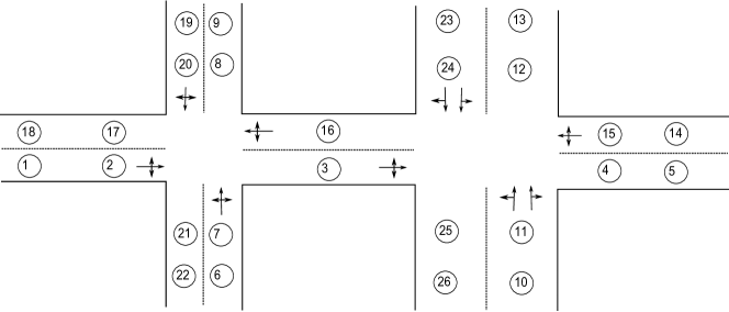
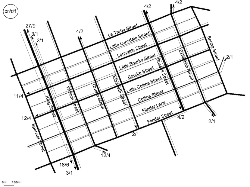
In this section we utilize an open source microscopic simulation package SUMO (Simulation of Urban MObility) [28] to study the above schemes in a small network of two intersections(Fig. 1) and in a large network(Fig. 2) that reassembles the Melbourne CBD (Australia) with about 70 intersections.

The small network has 2 junctions consisting of several in-roads (numbered from 1 to 26 on the figure Fig. 1). All the roads have bi-directional traffic with the North-South road going through the right intersection having double lanes. Direction of traffic movements on this network is indicated on each in-road leading to the junctions. The ingress queues, where vehicles enter the network, are assumed to be infinite and represented by a set of long links (i.e. links $\{1,18,9,19,13,23,5,14,10,26,6,22\}$ on Fig. 1). The cars immediately appear on the connecting in-roads inside the network, which are of finite capacity. Since the ingress queues are infinitely large, vehicles can enter the network even when there is a heavy congestion on the bottleneck link. All other links (i.e. links$\{2,3,4,7,8,11,12,20,21,24,25\}$ on Fig. 1) have the same length at $375$ meters which can accommodate maximum $50$ cars per lane.

The topology of the large CBD Melbourne network is shown in Fig. 2. It consists of $73$ intersections and $266$ links. Most of the roads are bi-directional except for Little Lonsdale Street, Little Bourke Street, Little Collins Street and Flinder Lane which only have a single lane mono-directional traffic. King Street and Russell Street are the biggest roads in this scenario, each is modeled as $3$ lanes each direction. Collins Street has one lane each direction. All other roads have two lanes each direction. The link lengths are varied between $106$ meters for the vertical links and $214$ meters and $447$ meters for the horizontal links except for the ingress links at the edges.

Results are given in terms of the total number of vehicles in the network and the congestion level which is the average number of congested links in large network after long simulation runs using the different control schemes. In all the studied scenarios, the exact queue lengths and turning fractions are observed directly from the simulation and used to make control decision in various policies. These variables are calculated using Matlab [19] based on the actual control algorithm and then are fed back into the SUMO simulation at every time step. We ignore switching times (i.e. transition between phases) in all control schemes in our study. This overhead can be incorporated into the simulation by extending the phase times. Nevertheless, the qualitative insights gained in this section would not change by that extension.

4.2 Performance Study

Below we evaluate the performance of our cyclic phase BackPressure scheme and compare it with other policies using fixed setting of routes in the studied networks using simulation. The cycle time of the cyclic phase BackPressure policy and the proportional policy were set to $30$ seconds, while the slot time of the BackPressure policy and the greedy policy were set to $10$ seconds in our simulation.

4.2.1 Small Network

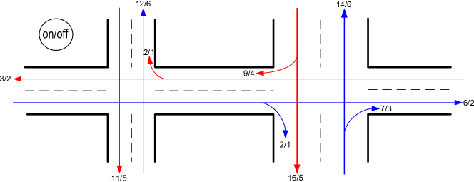
First, we study a small network scenario, for which the turning information and the arrival rates are indicated in Fig. 3. In particular, the arrows indicate 10 routes with direction and demands (cars/minutes) in the peak and off-peak (i.e. on/off) time periods as shown in Fig. 3. The $\eta$ value introduced in (7) was set to $2.5$. The main traffic flows are the ones with North-South direction of the second junction. The two BackPressure policies give the majority of service time to the North-South phase of that junction which leads to heavy congestion on links 1, 2, 3, 14 and 15. On the other hand, the proportional policy and greedy policy put more balance between the service times depending on the queue lengths which creates more congestion in the North-South direction at the cost of having less congestion in East-West direction.

Figure 3: Small network with demands.

Figure 4: Throughput for the small network using different policies. Cycle time for the cyclic phase BackPressure policy and the proportional policy is 30 seconds. Slot time for the BackPressure policy and the greedy policy is 10 seconds.

Figure 5: Congestion of bottleneck link for the small network using different policies. Cycle time for the cyclic phase BackPressure policy and the proportional policy is 30 seconds. Slot time for the BackPressure policy and the greedy policy is 10 seconds.

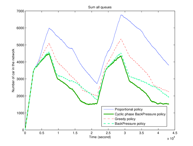
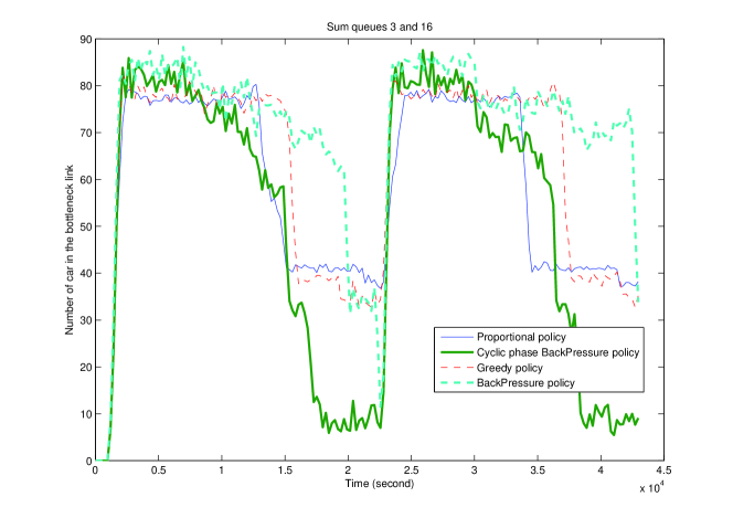
Results are shown in Fig. 4 and Fig. 5 where the total number of vehicles in the network and in the congested link between the two junctions are plotted over time. Note that there are two in-roads between the two intersections but only link 3 is congested due to large traffic flows in the North-South direction at the second intersection.

Note that Figs 4 and 5 were based on the number of cars present at the times when control decisions were made which is $30$ seconds for cyclic phase BackPressure and proportional policies. In contrast, the average travel time depends on the waiting time on individual link which is an integral of queue size over continuous time. For this reason, intermediate queue size was also measured at 10 s intervals in the simulation, and the results differed by less than 2% in compare with the coarse sampling at once per cycle assuming linear interpolation. The resulting travel time values are reported in the next sub-section 4.3.

Observe that the cyclic phase BackPressure control yields a lower number of total vehicles present in the network and thus results in higher number of vehicles reaching their destination (i.e. increased network throughput) during the whole simulation. This is due to the fact that in the two BackPressure control schemes when the bottleneck link (link 3) is congested, less green time will be allocated to the East-West direction at the first junction. As a result more traffic can move through the North-South direction and the impact of a spill back from the second junction on the overall network throughput decreases. Similarly, the BackPressure policy also outperforms the proportional policy and the greedy policy, since those two schemes allocate similar amount of green time to the East-West direction at the first junction despite the presence of a spilled back traffic and thus waste some of the green time.

4.2.2 Large Melbourne CBD network

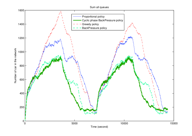
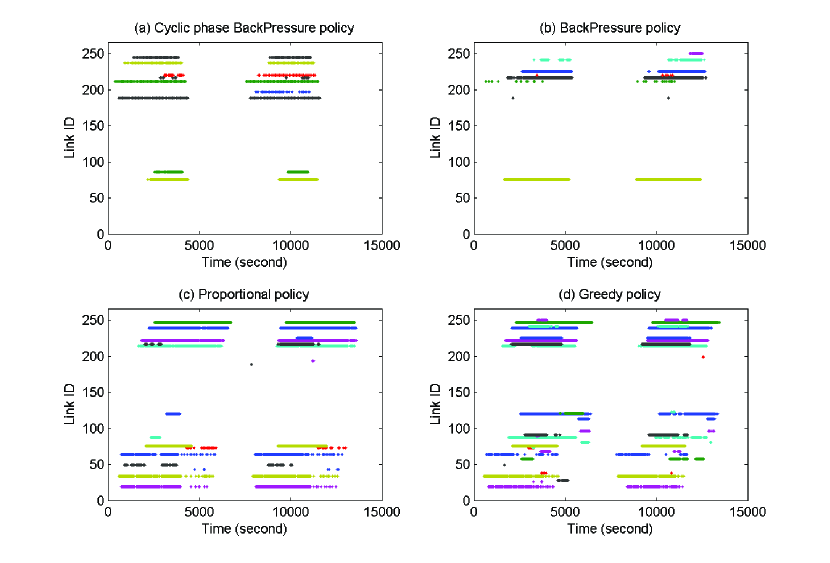
A similar study is performed with a large network with its turning information and arrival rates indicated in Fig. 2. The parameter $\eta$ is once again set to $2.5$. In this setting, the King Street has the largest flows, thus, any flow that shares an intersection with King Street tends to be under-served especially the intersection between King Street and Lonsdale Street and the intersection between King Street and Bourke Street. Generally in the peak period, congestion in any link will cause spill-back which leads to further congestion in the neighbouring junctions. This can only be recognized by the two BackPressure policies through comparing the in-road $i$ and out-road $i^{\prime}$, and more service will be allocated in this case to traffic flows on the less congested directions. In contrast, the proportional policy and the greedy policy only consider the queue lengths present at in-road $i$, and may waste some green time to the congested direction where traffic comes to a standstill due to the spill back.

Results for this scenario are shown in Fig. 6 and Fig. 7. As shown in Fig. 6 the cyclic phase BackPressure policy has the lowest total number of vehicles in the network, thus it provides the highest throughput, whereas the second highest throughput is provided by the BackPressure policy. Similarly to the previous scenario, the two BackPressure policies outperform the other two policies in case of heavy congestion because they take into account downstream queue lengths, and thus allocate resources (i.e. service phases) more efficiently.

Fig. 7 plots the congested link over time. Herein a link is said to be congested at a certain time if its queue length is more than $85\%$ of the link capacity. It is clear that the two BackPressure policies reduce the number of congested links significantly (i.e. less number of vehicles inside the network) resulting in higher network throughput.

Figure 6: Throughput for the large network using different policies. Cycle time for the cyclic phase BackPressure policy and the proportional policy is 30 seconds. Slot time for the BackPressure policy and the greedy policy is 10 seconds.

Figure 7: Congestion level for the large network using different policies. Cycle time for the cyclic phase BackPressure policy and the proportional policy is 30 seconds. Slot time for the BackPressure policy and the greedy policy is 10 seconds.

4.3 Experimental Parameter Design

The cycle length in the cyclic phase BackPressure policy and the proportional policy and the frequency of making decision in the BackPressure policy and the greedy policy play a crucial role in the performance of the control scheme. A long cycle length or the low frequency of making decision may be less efficient due to the fact that the queue might be depleted before the end of the service time. In the other hand, a short cycle length may reduce the overall capacity since the vehicles have to stop and accelerate more often. Note that the latter is in fact represents a switching cost between phases even though the amber traffic signal is not considered here. This subsection investigates the impact of the cycle time and decision making frequency on the throughput and congestion level of each scheme. We study both network topologies (the small network and the large CBD network) under the similar demand levels as in the previous subsection with different cycle times and decision frequencies. Particularly, for the cyclic phase BackPressure policy and the proportional policy, the cycle length is set to $\{30,60,90,120\}$ seconds, and for the BackPressure policy and the greedy policy, a decision is made every $\{10,30,60,90\}$ seconds, respectively.

4.3.1 Small Network

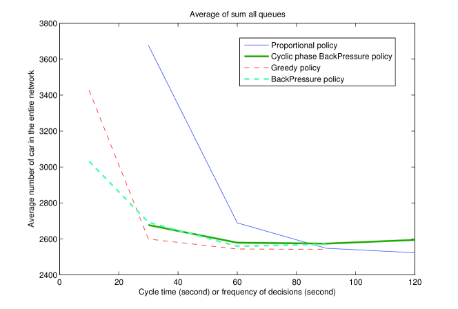
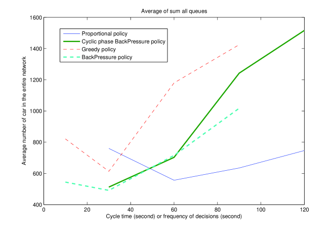
For small network, the results are presented in Fig. 8, Fig. 9, and Fig. 10. Fig. 8 shows the average number of vehicles in the network plotted against different cycle times. Because vehicle does not disappear and stays in the network until it exists, lower number of vehicles in the network equates to higher throughput of the same demand. In this scenario, all of the studied policies provide a similar throughput using their corresponding best setting. Furthermore, it can be observed that in congested network higher cycle times tend to have better throughput because the traffic flows are less interrupted by the switching between phases. Nevertheless, the proposed cyclic phase BackPressure is less sensitive to the changes of cycle time while producing a compatible throughput.

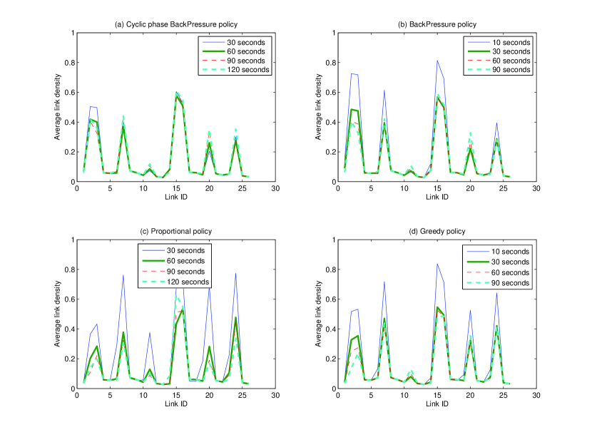
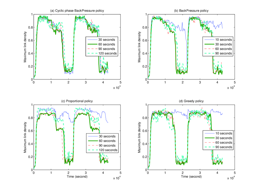
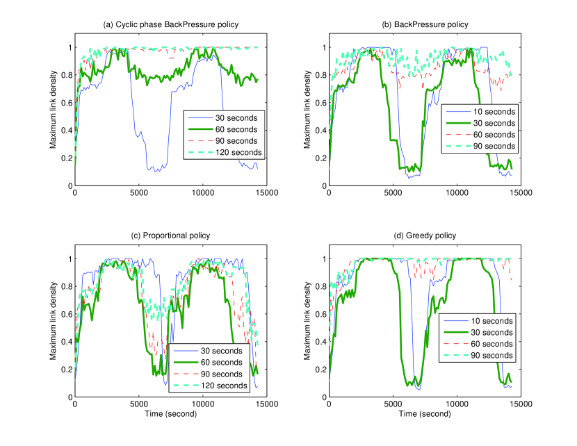
Fig. 9 plots the average link densities versus link ID. It shows that congestions occur in the same set of links throughout all of the studied policies. In overall, the cyclic phase BackPressure policy and the proportional policy have lower link density than the other two policies. Fig. 10 shows the maximum link density over time pointing to when the congestions occur in the network. In all cases, congestions appear during the peak period and some portion of time during the off-peak period before the build-up traffic can be substantially drained. However, when the cycle time or the decision frequency is set too small (e.g. 10 seconds for the BackPressure policy and the greedy policy and 30 seconds for the cyclic phase BackPressure policy and the proportional policy), the congestions are not able to cleared at all except for our cyclic phase BackPressure policy.

Figure 8: Throughput vs cycle time/frequency of decision for the small network.

Figure 9: Average link density for the small network.

Figure 10: Maximum link density for the small network.

4.3.2 Large Melbourne CBD Network

The impact of the cycle time and frequency of decision making on network throughput and congestion level using different policies for a large network are investigated and discussed in this subsection. The results are shown in Fig. 11, Fig. 12 and Fig. 13.

The average number of vehicles in the network for each setting is presented in Fig. 11. Unlike the results in the small network, there clearly exists an optimal value for the cycle length or decision making frequency of each policy. In particular the optimal cycle length for proportional policy is $60$ seconds, while the optimal cycle length/decision frequency for all other policies is $30$ seconds.

	Proportional	Cyclic phase BP	Greedy	BP
Avg. travel time	478.0	409.6	514.0	408.5

Table 1: Average travel time (in seconds) for the Melbourne CBD network using optimal setting for each policy (i.e. 60 seconds cycle length for the proportional policy, and 30 seconds cycle length for all other policies).

Observe that the optimal cycle length in the large network scenario is shorter than that of the small network, which can be explained by shorter link lengths and larger number of intersections on any route. Both increase the interdependency between intersections and their performance as arriving traffic into any internal intersection is an output traffic from the others.

Furthermore, the average travel time of each policy in their best setting of cycle length and decision making frequency is shown in Table 1. There is a strong correlation between the average number of vehicles in the network and average travel time through that network. In particular, the higher number of vehicles in the network results in the longer travel time and vice versa. It can be seen that the proposed cyclic phase BackPressure policy has a competitive average travel time between all the considered policies, and the results show that the BackPressure-based policies yield a significantly better average travel time than that of the greedy policy. Note that this better average travel time has been achieved with the control decisions using the queue size measurements at discrete time intervals (once in every cycle) only as explained earlier.

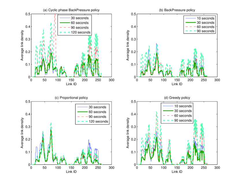
Fig. 12 plots the average link densities against the link ID. It shows that the congestion area is varied with different policy and with different parameter settings. Any cycle length/decision frequency setting other than the optimal setting obviously increases the congestion greatly.

Finally, Fig. 13 shows the maximum link density over time. The cycle length plays a vital role to prevent congestion in this scenario. In the cyclic phase BackPressure policy, the $30$ second cycle length is undoubtedly outstanding. In other policies, the small cycle lengths are seemed to be better due to the short link lengths.

Figure 11: Throughput vs cycle time/frequency of decision for the large network.

Figure 12: Average link density for the large network.

Figure 13: Maximum link density for the large network.

5 Conclusion

We proposed in this paper a novel decentralized signal control strategy based on the so-called BackPressure policy that does not require any $a~{}priori$ knowledge of the traffic demand and only needs information (i.e. queue size) that is local to the intersection. In contrast to other existing BackPressure-based policies in which phases can form an erratic and unpredictable order resulting in potential unsafe operation, our scheme allocates non-zero amount of time to each phases within the cycle, thus repeating them in a cyclic manner. Furthermore, unlike all the other existing Backpressure-based policies, no knowledge of the local turn ratios (turning fractions) is required in our control strategy. Instead any unbiased estimator of the turning fractions can be utilized in the proposed scheme. We have formally proved the stability results of the proposed signal control policy even though the controllers are reacting based only on local information and demand in an distributed manner. The stability results indicate that our policy is stable for the largest possible set of arrival rates (or demand) that will provide sufficient throughput even in congested network.

Using simulation, we compared our cyclic phase BackPressure performance against other well-known policies in terms of network throughput and congestion level using both small and large network topology with fixed routings. The results showed that our cyclic phase BackPressure policy tends to outperform other distributed polices both in terms of throughput and congestion. Although the performance of each policy varies widely depending on the parameter setting such as cycle length or decision frequency, under the optimal setting among the cases studied, the BackPressure with cyclic and non-cyclic operation have better throughput in compare with the other policies.

There are still many issues, such as non-constant switching times, finite link travel time and link capacity etc. that have not been considered here and will be a subject of future work.

Appendix A Estimation of Turning Fractions

An important aspect not addressed in the previous studies applying back pressure is the estimation of traffic turning fractions. Previous studies have either assumed the turning fractions are either explicitly known or have been calculated prior to the implementation of the policy.

Here we emphasize that the turning fractions can be estimated using recent locally calculated information about traffic flows. For instance, if we form an estimate on the turning fractions based on the last $k$ service cycles

$$\bar{q}_{ii^{\prime}}(t)=\frac{1}{k}\sum_{\kappa=1}^{k}\hat{p}_{ii^{\prime}}(t-{\kappa}),$$ (18)

where $\hat{p}_{ii^{\prime}}(t)$ denotes the measurement result for $p_{ii^{\prime}}(t)$. If $Q_{i}(t)=0$ then any estimate may be used to define $p_{ii^{\prime}{}}(t)$. Given that turning fractions are stationary and independent of queue sizes, these estimates form an unbiased estimate of the underlying turning probabilities as long as the measurement error in $\hat{p}_{ii^{\prime}}(t)$ has zero mean, since then

$$\bar{p}_{ii^{\prime}}={\mathbb{E}}[\bar{q}_{ii^{\prime}}(t)|Q_{i}(t)>0].$$ (19)

Other rules incorporating historical data or more recent data could also be considered here. What is necessary is that $\bar{q}_{ii^{\prime}}(t)$ provides an unbiased estimate of the underlying turning fractions of the vehicles for non-empty queues. It is even possible to use an inconsistent estimate of the turning fractions or for the proportions to change on a larger time scale, as long as the estimate is unbiased, independent of (the history of) $Q(t)$.

Appendix B Proof of the main stability result

In this section we prove Theorem 1. In order to that, we have to clarify some assumptions made about the stochastic elements of our model and provide some technical lemmas which are proven in a supplementary document together with Proposition 1.

B.1 Assumptions

1. The number of cars that can be served from any in-road within a traffic cycle is bounded,

   $$S_{\max}=\max_{t\in{\mathbb{Z}}_{+},i\in{\mathcal{I}}}S_{i}(t)<\infty.$$ (20)

2. $(p_{ii^{\prime}}(t):ii^{\prime}\in{\mathcal{L}})$ is stationary and independent of queue lengths $(Q_{i}(\tau):i\in{\mathcal{I}})$ and the number of cars served at each queue $(S_{i}(\tau):i\in{\mathcal{I}})$ for all $\tau\leq t$.

3. The matrix $I-\bar{p}$ is invertible. Thus we have, for $ii^{\prime}\in{\mathcal{L}}$

   $${\mathbb{E}}\left[S_{i}(t)p_{ii^{\prime}}(t)|Q(t)\right] =\sum_{\sigma\in{\mathcal{S}}_{j}}\sigma_{i}P^{j}_{\sigma}(t)\bar{p}_{ii^{\prime}}$$ (21)

   $${\mathbb{E}}\left[S_{i}(t)\wedge Q_{i}(t)p_{ii^{\prime}}(t)|Q(t)\right] ={\mathbb{E}}\left[S_{i}(t)\wedge Q_{i}(t)|Q(t)\right]\bar{p}_{ii^{\prime}}.$$ (22)

4. The number of arrival $(A_{i}(t):t\in{\mathbb{Z}}_{+}^{I})$ is independent of the state of the queues in the road traffic network. Thus the average arrival rate into each junction can be defined as

   $$\bar{a}_{i}(t)={\mathbb{E}}[A_{i}(t)].$$ (23)

5. The error term in the queue size measurement, $\delta(t)$ is bounded, i.e. $$|\delta_{i}(t)|\leq\delta_{\text{max}}\quad\forall i\in{\mathcal{I}}.$$ (24)

B.2 Lemmas

In this section, we will prove a number of additional lemmas that are required for the main proofs. The first lemma describes the difference of the weights caused by the error in measurement, whereas the second describes a general result on weights. The third lemma is a consquence of them, introducing a bound which is used multiple times in proving later statements.

Lemma 1.

$$w_{\sigma}(Q(t))=w_{\sigma}(\hat{Q}(t))-w_{\sigma}(\delta(t)),$$ (25) where $w_{\sigma}(Q(t))$ is defined according to (6).

Proof.

This statement is a straightforward consequence of the definition of the weights and the measurement error given in (1) and (6). Namely,

$$w_{\sigma}(Q(t)) =\sum_{i\in j}\sigma_{i}\left(Q_{i}(t)-\sum_{i^{\prime}:ii^{\prime}\in{\mathcal{L}}}\bar{q}_{ii^{\prime}}(t)Q_{i^{\prime}}(t)\right)$$ (26)

$$=\sum_{i\in j}\sigma_{i}\left(\left(\hat{Q}_{i}(t)-\epsilon_{i}(t)\right)-\sum_{i^{\prime}:ii^{\prime}\in{\mathcal{L}}}\bar{q}_{ii^{\prime}}(t)\left(\hat{Q}_{i^{\prime}}(t)-\delta_{i^{\prime}}(t)\right)\right)$$

$$=\sum_{i\in j}\sigma_{i}\left(\hat{Q}_{i}(t)-\sum_{i^{\prime}:ii^{\prime}\in{\mathcal{L}}}\bar{q}_{ii^{\prime}}(t)\hat{Q}_{i^{\prime}}(t)\right)$$

$$-\sum_{i\in j}\sigma_{i}\left(\delta_{i}(t)-\sum_{i^{\prime}:ii^{\prime}\in{\mathcal{L}}}\bar{q}_{ii^{\prime}}(t)\delta_{i^{\prime}}(t)\right)$$

$$=w_{\sigma}(\hat{Q}(t))-w_{\sigma}(\delta(t)).$$

∎

Lemma 2.

Given weights $(w_{y}:y\in{\mathcal{Y}})$ with elements indexed by finite set ${\mathcal{Y}}$, we consider $Y$ a random variable with the following probability of event $y$:

$$P_{y}=\frac{e^{\eta w_{y}}}{\sum_{y^{\prime}\in{\mathcal{Y}}}e^{\eta w_{y^{\prime}}}}$$ (27)

then, the expected value of the weights $w$ under this distribution obey the following inequality

$${\mathbb{E}}w_{Y}\geq\max_{y\in{\mathcal{Y}}}w_{y}-\frac{1}{\eta}\log|{\mathcal{Y}}|.$$ (28)

Proof.

In the following inequality, we note that the entropy of a distribution $H(P)=-{\mathbb{E}}\log P(Y)$ is maximized by a uniform distribution on ${\mathcal{Y}}$, $H(U)=\log|{\mathcal{Y}}|$.

$${\mathbb{E}}w_{Y}= \frac{1}{\eta}\log\left(\sum_{y\in{\mathcal{Y}}}e^{\eta w_{y}}\right)+\frac{1}{\eta}{\mathbb{E}}\log P(Y)\geq\frac{1}{\eta}\log\left(\sum_{y\in{\mathcal{Y}}}e^{\eta w_{y}}\right)-\frac{1}{\eta}\log{|{\mathcal{Y}}|}$$

$$\geq \frac{1}{\eta}\log\Big{(}e^{\eta\max_{y\in{\mathcal{Y}}}w_{y}}\Big{)}-\frac{1}{\eta}\log{|{\mathcal{Y}}|}=\max_{y\in{\mathcal{Y}}}w_{y}-\frac{1}{\eta}\log|{\mathcal{Y}}|,$$

as required. ∎

Lemma 3.

$$\sum_{\sigma\in{\mathcal{S}}_{j}}P^{j}_{\sigma}w_{\sigma}\left(\hat{Q}(t)\right)\geq\max_{\sigma\in{\mathcal{S}}_{j}}\Big{\{}w_{\sigma}\left(Q(t)\right)\Big{\}}-\delta_{\max}S_{\max}|{\mathcal{I}}|-\frac{1}{\eta}\log|{\mathcal{S}}_{j}|.$$ (29)

Proof.

We can prove this statement by applying Lemma 2 to $w_{\sigma}(\hat{Q}(t))$ , expanding the terms according to Lemma 1 and using the bound on $\delta(t)$ in (24).

$$\sum_{\sigma\in{\mathcal{S}}_{j}}P^{j}_{\sigma}w_{\sigma}(\hat{Q}(t)) ={\mathbb{E}}w_{\sigma}(\hat{Q}(t))\geq\max_{\sigma\in{\mathcal{S}}_{j}}\Big{\{}w_{\sigma}\left(\hat{Q}(t)\right)\Big{\}}-\frac{1}{\eta}\log|{\mathcal{S}}_{j}|$$ (30)

$$\geq\max_{\sigma\in{\mathcal{S}}_{j}}\Big{\{}w_{\sigma}\left(Q(t)\right)+w_{\sigma}\left(\delta(t)\right)\Big{\}}-\frac{1}{\eta}\log|{\mathcal{S}}_{j}|$$

$$\geq\max_{\sigma\in{\mathcal{S}}_{j}}\Big{\{}w_{\sigma}\left(Q(t)\right)\Big{\}}+\min_{\sigma\in{\mathcal{S}}_{j}}\Big{\{}w_{\sigma}\left(\delta(t)\right)\Big{\}}-\frac{1}{\eta}\log|{\mathcal{S}}_{j}|$$

$$\geq\max_{\sigma\in{\mathcal{S}}_{j}}\Big{\{}w_{\sigma}\left(Q(t)\right)\Big{\}}-\delta_{\max}S_{\max}|{\mathcal{I}}|-\frac{1}{\eta}\log|{\mathcal{S}}_{j}|$$

∎

Lemma 4 and Lemma 5 introduce bounds on the increments of the square of the queue sizes and their conditional expectations.

Lemma 4.

There exists a constant $K_{0}\geq 0$ such that our queue size process, (5), obeys the bound

$$\frac{1}{2}Q_{i}(t+1)^{2}-\frac{1}{2}Q_{i}(t)^{2}\leq Q_{i}(t)\left(A_{i}(t)-S_{i}(t)+\sum_{i^{\prime}:i^{\prime}i\in{\mathcal{L}}}S_{i^{\prime}}(t)p_{i^{\prime}i}(t)\right)+K_{0}.$$ (31)

Proof.

Firstly, the following bound holds for the queue size process, (5).

$$Q_{i}(t+1) =Q_{i}(t)-S_{i}(t)\wedge Q_{i}(t)+A_{i}(t)+\sum_{i^{\prime}:i^{\prime}i\in{\mathcal{L}}}[S_{i^{\prime}}(t)\wedge Q_{i^{\prime}{}}(t)]p_{i^{\prime}i}(t)$$

$$\leq Q_{i}(t)-S_{i}(t)\wedge Q_{i}(t)+A_{i}(t)+\sum_{i^{\prime}:i^{\prime}i\in{\mathcal{L}}}S_{i^{\prime}}(t)p_{i^{\prime}i}(t)$$

$$\leq\begin{cases}Q_{i}(t)-S_{i}(t)+A_{i}(t)+\sum_{i^{\prime}:i^{\prime}i\in{\mathcal{L}}}S_{i^{\prime}}(t)p_{i^{\prime}i}(t),&\text{if }Q_{i}(t)\geq S_{i}(t),\\ A_{i}(t)+\sum_{i^{\prime}:i^{\prime}i\in{\mathcal{L}}}S_{i^{\prime}}(t)p_{i^{\prime}i}(t),&\text{otherwise}.\end{cases}$$ (32)

Let’s consider the two cases above. Firstly, if $Q_{i}(t)<S_{i}(t)$ then, and according to the above bound, we have

$$\frac{1}{2}Q_{i}(t+1)^{2}-\frac{1}{2}Q_{i}(t)^{2}\leq \frac{1}{2}Q_{i}(t+1)^{2}\leq\frac{1}{2}\left(A_{i}(t)+\sum_{i^{\prime}:i^{\prime}i\in{\mathcal{L}}}S_{i^{\prime}}(t)p_{i^{\prime}i}(t)\right)^{2}$$

$$\leq \frac{1}{2}\left(a_{max}+S_{\max}(|{\mathcal{I}}|+1)\right)^{2}$$

$$\leq -Q_{i}(t)\left(S_{i}(t)-A_{i}(t)-\sum_{i^{\prime}:i^{\prime}i\in{\mathcal{L}}}S_{i^{\prime}}(t)p_{i^{\prime}i}(t)\right)$$ (33)

$$+S_{\max}\left(a_{max}+S_{\max}(|{\mathcal{I}}|+1)\right)$$ (34)

$$+\frac{1}{2}\left(a_{max}+S_{\max}(|{\mathcal{I}}|+1)\right)^{2}.$$

In the final inequality, we use the fact that the term, (33), is bounded by the term (34).

Secondly, if $Q_{i}(t)\geq S_{i}(t)$ then, according to (32),

$$\frac{1}{2}Q_{i}(t+1)^{2}-\frac{1}{2}Q_{i}(t)^{2}\leq -Q_{i}(t)\left(S_{i}(t)-A_{i}(t)-\sum_{i^{\prime}:i^{\prime}i\in{\mathcal{L}}}S_{i^{\prime}}(t)p_{i^{\prime}i}(t)\right)$$

$$+\frac{1}{2}\left(S_{i}(t)-A_{i}(t)-\sum_{i^{\prime}:i^{\prime}i\in{\mathcal{L}}}S_{i^{\prime}}(t)p_{i^{\prime}i}(t)\right)^{2}$$

$$\leq -Q_{i}(t)\left(S_{i}(t)-A_{i}(t)-\sum_{i^{\prime}:i^{\prime}i\in{\mathcal{L}}}S_{i^{\prime}}(t)p_{i^{\prime}i}(t)\right)$$

$$+\frac{1}{2}\left(a_{\max}+(|{\mathcal{I}}|+1)S_{\max}\right)^{2}.$$

Thus defining

$$K_{0}=\frac{1}{2}\left(a_{\max}+(|{\mathcal{I}}|+1)S_{\max}\right)^{2}+S_{\max}\left(a_{max}+S_{\max}(|{\mathcal{I}}|+1)\right),$$

we see that in both cases, above, we have the required bound

$$\frac{1}{2}Q_{i}(t+1)^{2}-\frac{1}{2}Q_{i}(t)^{2}\leq Q_{i}(t)\left(A_{i}(t)-S_{i}(t)+\sum_{i^{\prime}:i^{\prime}i\in{\mathcal{L}}}S_{i^{\prime}}(t)p_{i^{\prime}i}(t)\right)+K_{0}.$$

∎

Lemma 5.

There exists a constant $K_{1}>0$ such that the following equality holds

$${\mathbb{E}}\left[Q_{i}(t)S_{i^{\prime}}(t)p_{i^{\prime}i}(t)\Big{|}Q(t),\delta(t)\right]\leq{\mathbb{E}}\Big{[}Q_{i}(t)\sum_{\sigma\in{\mathcal{S}}_{j}(i^{\prime})}\sigma_{i^{\prime}{}}(t)P^{j(i^{\prime})}_{\sigma}\bar{q}_{i^{\prime}i}(t)\Big{|}Q(t),\delta(t)\Big{]}+K_{1}.$$ (35)

Proof.

First let us suppose that the queue has been empty over the last $k$ time steps. Then, since a bounded number of cars arrive at the queue per traffic cycle, the queue size $Q_{i}(t)$ must be less than $(a_{\max}+\sigma_{max}|{\mathcal{L}}|)$. Clearly the above bound holds for any, $Q_{i}(t)\leq K_{1}=S_{\max}(a_{\max}+\sigma_{max}|{\mathcal{L}}|)$. Now lets suppose $Q_{i}(t)\geq K_{1}$, we can take $Q_{i}(t)$ out the conditional expectation because it is known

$${\mathbb{E}}[Q_{i}(t)S_{i^{\prime}}(t)p_{i^{\prime}i}(t)|Q(t),\delta(t)]=Q_{i}(t){\mathbb{E}}[S_{i^{\prime}}(t)p_{i^{\prime}i}(t)|Q(t),\delta(t)].$$

The proportion of traffic $p(t)$ is independent of $S(t)$ and of $Q(t)$. So the expectation of $p_{i^{\prime}i}(t)$ given $Q(t)$ (and $S(t)$) is its mean $\bar{p}_{ii^{\prime}}$. So

$${\mathbb{E}}[S_{i^{\prime}}(t)p_{i^{\prime}i}(t)|Q(t),\delta(t)]={\mathbb{E}}[S_{i^{\prime}}(t)\bar{p}_{i^{\prime}i}|Q(t),\delta(t)]=\bar{p}_{i^{\prime}i}{\mathbb{E}}[S_{i^{\prime}}(t)|Q(t),\delta(t)].$$

Also (3) implies

$${\mathbb{E}}[S_{i^{\prime}}(t)|Q(t),\delta(t)]=\sum_{\sigma\in{\mathcal{S}}_{j(i^{\prime})}}\sigma_{i^{\prime}}P^{j(i^{\prime})}_{\sigma}.$$

Also since $q_{i^{\prime}i}(t)$ is an unbiased estimate of $p_{i^{\prime}i}$ at time $t$, and independent of $Q(t)$ by assumption,

$$\bar{p}_{i^{\prime}i}={\mathbb{E}}[q_{i^{\prime}i}(t)|Q(t)].$$

Substituting this all back in, we have

$${\mathbb{E}}[Q_{i}(t)S_{i^{\prime}}(t)p_{i^{\prime}i}(t)|Q(t),\delta(t)] =Q_{i}(t)\bar{p}_{i^{\prime}i}{\mathbb{E}}[S_{i^{\prime}}(t)|Q(t),\delta(t)]$$

$$=Q_{i}(t){\mathbb{E}}[q_{i^{\prime}i}(t)|Q(t),\delta(t)]\sum_{\sigma\in{\mathcal{S}}_{j(i^{\prime})}}\sigma_{i^{\prime}}P^{j(i^{\prime})}_{\sigma}$$

$$={\mathbb{E}}\Big{[}Q_{i}(t)\sum_{\sigma\in{\mathcal{S}}_{j}(i^{\prime})}{\sigma}_{i^{\prime}{}}P^{j(i^{\prime})}_{\sigma}\bar{q}_{i^{\prime}i}(t)\Big{|}Q(t),\delta(t)\Big{]},$$

thus the above inequality also holds in the case $Q_{i}(t)>K_{1}$ as required. ∎

Lemma 6 indicates an allowed reordering of terms.

Lemma 6.

The following equality holds for each measured queue size vector,

$$\sum_{i\in{\mathcal{I}}}\hat{Q}_{i}(t)\left(\sum_{\sigma\in{\mathcal{S}}_{j(i)}}\sigma_{i}P^{j(i)}_{\sigma}(t)-\sum_{i^{\prime}:(i^{\prime},i)\in{\mathcal{L}}}\sum_{\sigma\in{\mathcal{S}}_{j^{\prime}(i^{\prime})}}\sigma_{i^{\prime}}P^{j(i^{\prime})}_{\sigma}\bar{q}_{i^{\prime}i}(t)\right)$$

$$=\sum_{k\in{\mathcal{J}}}\sum_{\sigma\in{\mathcal{S}}_{k}}P^{k}_{\sigma}(t)\sum_{i\in k}\sigma_{i}\left(\hat{Q}_{i}(t)-\sum_{i^{\prime}:ii^{\prime}\in{\mathcal{L}}}\hat{Q}_{i^{\prime}}(t)\bar{q}_{ii^{\prime}}(t)\right).$$

Proof.

Although the following set of equalities is some what lengthy, the premise is fairly simple. We want to change to order of summation so that we first sum over junctions ${\mathcal{J}}$ instead of first summing over in-roads ${\mathcal{I}}$. These manipulations are as follows

$$\sum_{i\in{\mathcal{I}}}\hat{Q}_{i}(t)\left(\sum_{\sigma\in{\mathcal{S}}_{j(i)}}\sigma_{i}P^{j(i)}_{\sigma}(t)-\sum_{i^{\prime}:(i^{\prime},i)\in{\mathcal{L}}}\sum_{\sigma\in{\mathcal{S}}_{j^{\prime}(i^{\prime})}}\sigma_{i^{\prime}}P^{j(i^{\prime})}_{\sigma}\bar{q}_{i^{\prime}i}(t)\right)$$

$$= \sum_{i\in{\mathcal{I}}}\sum_{k\in{\mathcal{J}}}\sum_{\sigma\in{\mathcal{S}}_{k}}\hat{Q}_{i}(t)\sigma_{i}P^{k}_{\sigma}(t){\mathbb{I}}[i\in k]-\sum_{i\in{\mathcal{I}}}\sum_{i^{\prime}:i^{\prime}i\in{\mathcal{L}}}\sum_{k\in{\mathcal{J}}}\sum_{\sigma\in{\mathcal{S}}_{k}}\hat{Q}_{i}(t)\sigma_{i^{\prime}}P^{k}_{\sigma}\bar{q}_{i^{\prime}i}(t){\mathbb{I}}[i^{\prime}\in k]$$

$$= \sum_{k\in{\mathcal{J}}}\sum_{\sigma\in{\mathcal{S}}_{k}}P^{k}_{\sigma}(t)\sum_{i\in{\mathcal{I}}}\hat{Q}_{i}(t)\sigma_{i}{\mathbb{I}}[i\in k]-\sum_{k\in{\mathcal{J}}}\sum_{\sigma\in{\mathcal{S}}_{k}}P^{k}_{\sigma}\sum_{i\in{\mathcal{I}}}\sum_{i^{\prime}:i^{\prime}i\in{\mathcal{L}}}\hat{Q}_{i}(t)\sigma_{i^{\prime}}\bar{q}_{i^{\prime}i}(t){\mathbb{I}}[i^{\prime}\in k]$$

$$= \sum_{k\in{\mathcal{J}}}\sum_{\sigma\in{\mathcal{S}}_{k}}P^{k}_{\sigma}(t)\left(\sum_{i\in k}\hat{Q}_{i}(t)\sigma_{i}-\sum_{i^{\prime}\in{\mathcal{I}}}\sum_{i:i^{\prime}i\in{\mathcal{L}}}\hat{Q}_{i}(t)\sigma_{i^{\prime}}\bar{q}_{i^{\prime}i}(t){\mathbb{I}}[i^{\prime}\in k]\right)$$

$$= \sum_{k\in{\mathcal{J}}}\sum_{\sigma\in{\mathcal{S}}_{k}}P^{k}_{\sigma}(t)\sum_{i\in k}\sigma_{i}\left(\hat{Q}_{i}(t)-\sum_{i^{\prime}:ii^{\prime}\in{\mathcal{L}}}\hat{Q}_{i^{\prime}}(t)\bar{q}_{ii^{\prime}}(t)\right).$$

In the first equality above, we expand brackets. In the second equality, we reorder the summation so we first sum over junctions and then over schedules. In the third and fourth equality, we collect together terms for each in-road. ∎

Our last lemma gives a bound on an optimization problem to be used later.

Lemma 7.

If ${a}+\epsilon\mathbf{1}\in{\mathcal{A}}$ then

$$\epsilon<\left(1-\frac{L}{T}\right)\min_{u\geq 0:\sum_{i\in{\mathcal{I}}}u_{i}=1}\left(\sum_{j\in{\mathcal{J}}}\max_{\sigma\in{\mathcal{S}}_{j}}\left\{w_{\sigma}\left(u\right)\right\}-\sum_{i\in{\mathcal{I}}}u_{i}\bar{a}_{i}(t)\right).$$

Proof.

By definition ${a}+\epsilon\mathbf{1}\in{\mathcal{A}}$ when there exists a positive vector $\rho=(\rho^{j}_{\sigma}:\sigma\in{\mathcal{S}}_{j},j\in{\mathcal{J}})$ and a positive vector $s=(s_{i}:i\in{\mathcal{I}})$ satisfying the constraints

$$a_{i}+\epsilon+\sum_{i^{\prime}:i^{\prime}i\in{\mathcal{L}}}s_{i^{\prime}}\bar{p}_{i^{\prime}i}<s_{i},$$ (36)

$$\sum_{\sigma\in{\mathcal{S}}_{j}} \rho^{j}_{\sigma}\leq 1-\frac{L}{T},\qquad s_{i}\leq\sum_{\sigma\in{\mathcal{S}}_{j}}\rho^{j}_{\sigma}\sigma_{i}$$ (37)

for each $j\in{\mathcal{J}}$ and $i\in j$. We can express (36) more concisely in vector form as $a+\epsilon\mathbf{1}<s^{\textsf{T}}(I-\bar{p})$. Notice the inverse of $(I-\bar{p})$ is the positive matrix $(I-\bar{p})^{-1}=I+\bar{p}+\bar{p}^{2}+...$ Thus we can equivalently express condition (36) as

$$(a+\epsilon\mathbf{1})^{\textsf{T}}(I-\bar{p})<s^{\textsf{T}}.$$ (38)

We can now observe that if we replace $s$ as above with

$$\tilde{s}_{i}=\sum_{\sigma\in{\mathcal{S}}_{j}}\rho^{j}_{\sigma}\sigma_{i}$$ (39)

then equations (36-37) must hold. In other words there exists a $\rho=(\rho^{j}_{\sigma}:\sigma\in{\mathcal{S}}_{j},j\in{\mathcal{J}})$ such that

$$a_{i}+\epsilon+\sum_{i^{\prime}:i^{\prime}i\in{\mathcal{L}}}\sum_{\sigma\in{\mathcal{S}}_{j(i^{\prime})}}\rho^{j(i^{\prime})}_{\sigma}\sigma_{i^{\prime}}\bar{p}_{i^{\prime}i} <\sum_{\sigma\in{\mathcal{S}}_{j}}\rho^{j}_{\sigma}\sigma_{i}, \text{for }i\in j,\text{ with }j\in{\mathcal{J}},$$ (40)

$$\sum_{\sigma\in{\mathcal{S}}_{j}} \rho^{j}_{\sigma}\leq 1-\frac{L}{T}, \text{for }j\in{\mathcal{J}}.$$ (41)

We now focus on the inequality (40). Rearranging it, the above holds when there exists $\rho$ such that

$$\epsilon <\min_{j\in{\mathcal{J}},i\in j}\left\{\sum_{\sigma\in{\mathcal{S}}_{j}}\rho^{j}_{\sigma}\sigma_{i}-\sum_{i^{\prime}:i^{\prime}i\in{\mathcal{L}}}\sum_{\sigma\in{\mathcal{S}}_{j(i^{\prime})}}\rho^{j(i^{\prime})}_{\sigma}\sigma_{i^{\prime}}\bar{p}_{i^{\prime}i}-a_{i}\right\},$$ (42)

$$\qquad\qquad\qquad\sum_{\sigma\in{\mathcal{S}}_{j}}\rho^{j}_{\sigma}\leq 1-\frac{L}{T}, j\in{\mathcal{J}}.$$ (43)

The above statement can only hold if it also holds when we maximize over $\rho$ thus the following must hold

$$\epsilon<\max_{\rho:\forall j\in{\mathcal{J}},\sum_{\sigma\in{\mathcal{S}}_{j}}\rho^{j}_{\sigma}\leq 1-L/T}\min_{j\in{\mathcal{J}},i\in j}\left\{\sum_{\sigma\in{\mathcal{S}}_{j}}\rho^{j}_{\sigma}\sigma_{i}-\sum_{i^{\prime}:i^{\prime}i\in{\mathcal{L}}}\sum_{\sigma\in{\mathcal{S}}_{j(i^{\prime})}}\rho^{j(i^{\prime})}_{\sigma}\sigma_{i^{\prime}}\bar{p}_{i^{\prime}i}-a_{i}\right\}.$$ (44)

Since the minimum of a finite set in ${\mathbb{R}}$ is equal to the minimum of the convex combinations of elements in that set,

$$\min_{i\in{\mathcal{I}}}\left\{\sum_{\sigma\in{\mathcal{S}}_{j(i)}}\rho^{j(i)}_{\sigma}\sigma_{i}-\sum_{i^{\prime}:i^{\prime}i\in{\mathcal{L}}}\sum_{\sigma\in{\mathcal{S}}_{j(i^{\prime})}}\rho^{j(i^{\prime})}_{\sigma}\sigma_{i^{\prime}}\bar{p}_{i^{\prime}i}-a_{i}\right\}$$

$$= \min_{u\geq 0:\sum_{i\in{\mathcal{I}}}u_{i}=1}\left\{\sum_{i\in{\mathcal{I}}}\sum_{\sigma\in{\mathcal{S}}_{j(i)}}\rho^{j(i)}_{\sigma}\sigma_{i}u_{i}-\sum_{i\in{\mathcal{I}}}\sum_{i^{\prime}:i^{\prime}i\in{\mathcal{L}}}\sum_{\sigma\in{\mathcal{S}}_{j(i^{\prime})}}\rho^{j(i^{\prime})}_{\sigma}\sigma_{i^{\prime}}\bar{p}_{i^{\prime}i}u_{i}-\sum_{i\in\in{\mathcal{I}}}a_{i}u_{i}\right\}.$$ (45)

Next by exactly the same argument used to prove Lemma 6, we have that

$$\sum_{i\in{\mathcal{I}}}\sum_{\sigma\in{\mathcal{S}}_{j(i)}}\rho^{j(i)}_{\sigma}\sigma_{i}u_{i}-\sum_{i\in{\mathcal{I}}}\sum_{i^{\prime}:i^{\prime}i\in{\mathcal{L}}}\sum_{\sigma\in{\mathcal{S}}_{j(i^{\prime})}}\rho^{j(i^{\prime})}_{\sigma}\sigma_{i^{\prime}}\bar{p}_{i^{\prime}i}u_{i}-\sum_{i\in{\mathcal{I}}}a_{i}u_{i}$$

$$= \sum_{k\in{\mathcal{J}}}\sum_{\sigma\in{\mathcal{S}}_{k}}\rho^{k}_{\sigma}\sum_{i\in k}\sigma_{i}\left(u_{i}-\sum_{i^{\prime}:ii^{\prime}\in{\mathcal{L}}}u_{i^{\prime}}\bar{p}_{ii^{\prime}}\right)-\sum_{i\in{\mathcal{I}}}a_{i}u_{i}.$$

Substituting this equality into (45), we have that (44) reads as

$$\epsilon<\max_{\rho:\forall j\in{\mathcal{J}},\sum_{\sigma\in{\mathcal{S}}_{j}}\rho^{j}_{\sigma}\leq 1-L/T}\min_{u\geq 0:\sum_{i\in{\mathcal{I}}}u_{i}=1}\left\{\sum_{k\in{\mathcal{J}}}\sum_{\sigma\in{\mathcal{S}}_{k}}\rho^{k}_{\sigma}\sum_{i\in k}\sigma_{i}\left(u_{i}-\sum_{i^{\prime}:ii^{\prime}\in{\mathcal{L}}}u_{i^{\prime}}\bar{p}_{ii^{\prime}}\right)-\sum_{i\in{\mathcal{I}}}a_{i}u_{i}\right\}.$$ (46)

Finally for any function $f(u,\rho)$, it holds that $\min_{u}\max_{\rho}f(u,\rho)\geq\max_{\rho}\min_{u}f(u,\rho)$. Thus if $\bar{a}+\epsilon\mathbf{1}\in{\mathcal{A}}$ then it must be true that

$$\epsilon<\min_{u\geq 0:\sum_{i\in{\mathcal{I}}}u_{i}=1}\max_{\rho:\forall j\in{\mathcal{J}},\sum_{\sigma\in{\mathcal{S}}_{j}}\rho^{j}_{\sigma}\leq 1-L/T}\left\{\sum_{k\in{\mathcal{J}}}\sum_{\sigma\in{\mathcal{S}}_{k}}\rho^{k}_{\sigma}\sum_{i\in k}\sigma_{i}\left(u_{i}-\sum_{i^{\prime}:ii^{\prime}\in{\mathcal{L}}}u_{i^{\prime}}\bar{p}_{ii^{\prime}}\right)-\sum_{i\in{\mathcal{I}}}a_{i}u_{i}\right\}.$$

Finally, we note that the above maximization over $\rho$ must be achieved at a value where, for each $j\in{\mathcal{J}}$, $\rho^{j}_{\sigma}=1-\frac{L}{T}$ for some $\sigma$, so

$$\epsilon<\left(1-\frac{L}{T}\right)\min_{u\geq 0:\sum_{i\in{\mathcal{I}}}u_{i}=1}\left\{\sum_{j\in{\mathcal{J}}}\max_{\sigma\in{\mathcal{S}}_{j}}\sum_{i\in j}\sigma_{i}\left(u_{i}-\sum_{i^{\prime}:ii^{\prime}\in{\mathcal{L}}}u_{i^{\prime}}\bar{p}_{ii^{\prime}}\right)-\sum_{i\in{\mathcal{I}}}a_{i}u_{i}\right\}.$$

∎

B.3 Proofs

We now provide a proof that the road traffic network is unstable whenever the arrival rates are outside the set $\bar{{\mathcal{A}}}$.

Proof of Proposition 1.

If $\bar{a}\notin\bar{{\mathcal{A}}}$ then there exists an $\epsilon>0$ where, for any vector $\rho=(\rho_{\sigma}^{j}:\sigma\in{\mathcal{S}}_{j},j\in{\mathcal{J}})$ and $s=(s_{i}:i\in{\mathcal{I}})$, satisfying

$$\sum_{\sigma\in{\mathcal{S}}_{j}} \rho^{j}_{\sigma}\leq 1-\frac{L}{T},\qquad\text{and}\qquad s_{i^{\prime}}\leq\sum_{\sigma\in{\mathcal{S}}_{j}}\rho^{j}_{\sigma}\sigma_{i^{\prime}}$$ (47)

for $j\in{\mathcal{J}}$ and ${i^{\prime}}\in{\mathcal{I}}$, and there exists an in-road $i$ such that

$$a_{i}-s_{i}+\sum_{i^{\prime}:i^{\prime}i\in{\mathcal{L}}}s_{i^{\prime}}\bar{p}_{i^{\prime}i} >\epsilon.$$ (48)

Consider any policy $P_{\sigma}$, and consider the average service devoted to each queue and the number of departures from each queue

$$\rho_{\sigma}^{j}(\tau)=\frac{1}{\tau}\sum_{t=1}^{\tau}P_{\sigma}^{j}(t)\quad\text{and}\quad s_{i}(\tau)=\frac{1}{\tau}\sum_{t=1}^{\tau}S_{i}(t).$$

Taking a suitable subsequence if necessary, the sequences $\rho_{\sigma}^{j}(t)$ and $s_{i}(t)$ must converge to some value $\rho_{\sigma}^{j}$ and $s_{i}$ satisfying condition (47). The long run queue size must converge to the average arrival minus the average departures. Thus we have that

$$\lim_{t\rightarrow\infty}\frac{Q^{\Sigma}(t)}{t}=\sum_{i\in{\mathcal{I}}}\left(\bar{a}_{i}+\sum_{i^{\prime}:i^{\prime}i\in{\mathcal{L}}}s_{i^{\prime}}\bar{p}_{i^{\prime}i}-s_{i}\right)>\epsilon.$$

In the above inequality, we note that each term in the above summation is positive since it is the limit of positive queue sizes and one of those terms in greater than $\epsilon$ by (48). Thus we see that for any policy there always exists a queue that is unstable: there exists a $t_{0}$ such that for all $t>t_{0}$

$$Q^{\Sigma}(t)>t\epsilon,$$

thus,

$$\lim_{\tau\rightarrow\infty}\frac{1}{\tau}\sum_{t=1}^{\tau}Q^{\Sigma}(t)\geq\lim_{\tau\rightarrow\infty}\frac{1}{\tau}\sum_{t=t_{0}}^{\tau}\epsilon t=\infty.$$

So, taking expectations, we see that the network must be unstable:

$$\limsup_{\tau\rightarrow\infty}{\mathbb{E}}\left[\frac{1}{\tau}\sum_{t=1}^{\tau}Q^{\Sigma}(t)\right]\geq{\mathbb{E}}\left[\liminf_{\tau\rightarrow\infty}\frac{1}{\tau}\sum_{t=1}^{\tau}Q^{\Sigma}(t)\right]=\infty.$$

In the last inequality we apply Fatou’s Lemma. ∎

B.4 Formal proof of Theorem 1

We now begin to develop the proof of Theorem 1. First, we require a bound on the change in the (euclidean) distance of our queue sizes from zero. This is proven in the following proposition.

Proposition 2.

There exists a constant $K^{*}$ such that

$$\sum_{i\in{\mathcal{I}}}{\mathbb{E}}\left[\frac{1}{2}Q_{i}(t+1)^{2}-\frac{1}{2}Q_{i}(t)^{2}\bigg{|}Q(t),\delta(t)\right]$$

$$\leq {\mathbb{E}}\left[\sum_{i\in{\mathcal{I}}}Q_{i}(t)\bar{a}_{i}(t)-\sum_{j\in{\mathcal{J}}}\sum_{\sigma\in{\mathcal{S}}_{j}}P^{j}_{\sigma}w_{\sigma}(Q(t))\Bigg{|}Q(t),\delta(t)\right]+K^{*}$$

where $w_{\sigma}(Q(t))$ is defined by (6).

Proof.

We can expand the left side through the following inequalities to reach the desired bound

$$\sum_{i\in{\mathcal{I}}}{\mathbb{E}}\left[\frac{1}{2}Q_{i}(t+1)^{2}-\frac{1}{2}Q_{i}(t)^{2}\bigg{|}Q(t),\delta(t)\right]$$

$$\leq \sum_{i\in{\mathcal{I}}}{\mathbb{E}}\left[Q_{i}(t)\left(A_{i}(t)-S_{i}(t)+\sum_{i^{\prime}:i^{\prime}i\in{\mathcal{L}}}S_{i^{\prime}}(t)p_{i^{\prime}i}(t)\right)\bigg{|}Q(t),\delta(t)\right]+K_{0}$$

$$\leq \sum_{i\in{\mathcal{I}}}{\mathbb{E}}\left[Q_{i}(t)\left(\bar{a}_{i}(t)-\sum_{\sigma\in{\mathcal{S}}_{j(i)}}{\sigma}_{i}P^{j(i)}_{\sigma}(t)+\sum_{i^{\prime}:i^{\prime}i\in{\mathcal{L}}}\sum_{\sigma\in{\mathcal{S}}_{j(i^{\prime})}}{\sigma}_{i^{\prime}}P^{j(i^{\prime})}_{\sigma}\bar{q}_{i^{\prime}i}(t)\right)\Bigg{|}Q(t),\delta(t)\right]+\tilde{K}$$

$$= {\mathbb{E}}\left[\sum_{i\in{\mathcal{I}}}Q_{i}(t)\bar{a}_{i}(t)\Bigg{|}Q(t),\delta(t)\right]+\tilde{K}$$

$$- {\mathbb{E}}\left[\sum_{i\in{\mathcal{I}}}\left(\hat{Q}_{i}(t)-\delta_{i}(t)\right)\left(\sum_{\sigma\in{\mathcal{S}}_{j(i)}}{\sigma}_{i}P^{j(i)}_{\sigma}(t)-\sum_{i^{\prime}:i^{\prime}i\in{\mathcal{L}}}\sum_{\sigma\in{\mathcal{S}}_{j(i^{\prime})}}{\sigma}_{i^{\prime}}P^{j(i^{\prime})}_{\sigma}\bar{q}_{i^{\prime}i}(t)\right)\Bigg{|}Q(t),\delta(t)\right]$$

$$\leq {\mathbb{E}}\left[\sum_{i\in{\mathcal{I}}}Q_{i}(t)\bar{a}_{i}(t)-\sum_{j\in{\mathcal{J}}}\sum_{\sigma\in{\mathcal{S}}_{j}}P^{j}_{\sigma}w_{\sigma}(\hat{Q}(t))\Bigg{|}Q(t),\delta(t)\right]+K^{*}.$$

The first inequality can be reached by using Lemma 4 to expand the recursion (5) for some constant $K_{0}>0$. Then by using the inequalities

$${\mathbb{E}}\left[Q_{i}(t)S_{i^{\prime}}(t)p_{i^{\prime}i}(t)\Big{|}Q(t),\delta(t)\right]\leq{\mathbb{E}}\Big{[}Q_{i}(t)\sum_{\sigma\in{\mathcal{S}}_{j(i^{\prime})}}{\sigma}_{i^{\prime}}P^{j(i^{\prime})}_{\sigma}\bar{q}_{i^{\prime}i}(t)\Big{|}Q(t),\delta(t)\Big{]}+K_{1}$$ (49)

and

$${\mathbb{E}}\left[Q_{i}(t)A_{i}(t)\Big{|}Q(t)\right]=Q_{i}(t)\bar{a}_{i}(t)$$ (50)

with rearranging we can further expand by taking constant $\tilde{K}=K_{0}+|{\mathcal{L}}|K_{1}$ for instance. (49) is proven in Lemma 5, whereas (50) holds by definition (23). The last inequality is given by swapping the order of summation inside the expectation from a summation over queues on in-roads ${\mathcal{I}}$ and then as a summation over schedules ${\mathcal{S}}_{j}$ to the other way around, and using the bound on the error terms in (24). By Lemma 6 and by the definition of the weights $w_{\sigma}(\hat{Q}(t))$ in (6), we have that

$$\sum_{i\in{\mathcal{I}}}\hat{Q}_{i}(t)\left(\sum_{\sigma\in{\mathcal{S}}_{j(i)}}{\sigma}_{i}P^{j(i)}_{\sigma}(t)-\sum_{i^{\prime}:i^{\prime}i\in{\mathcal{L}}}\sum_{\sigma\in{\mathcal{S}}_{j(i^{\prime})}}{\sigma}_{i^{\prime}}P^{j(i^{\prime})}_{\sigma}\bar{q}_{i^{\prime}i}(t)\right)$$

$$= \sum_{k\in{\mathcal{J}}}\sum_{\sigma\in{\mathcal{S}}_{k}}P^{k}_{\sigma}(t)\sum_{i\in k}{\sigma}_{i}\left(\hat{Q}_{i}(t)-\sum_{i^{\prime}:ii^{\prime}\in{\mathcal{L}}}\hat{Q}_{i^{\prime}}(t)\bar{q}_{ii^{\prime}}(t)\right)$$

$$= \sum_{k\in{\mathcal{J}}}\sum_{\sigma\in{\mathcal{S}}_{k}}P^{k}_{\sigma}w_{\sigma}(\hat{Q}(t)).$$

Furthermore we can bound the extra term arising from the measurement error as $\displaystyle{\mathbb{E}}\left[\sum_{i\in{\mathcal{I}}}\delta_{i}(t)\left(\sum_{\sigma\in{\mathcal{S}}_{j(i)}}{\sigma}_{i}P^{j(i)}_{\sigma}(t)-\sum_{i^{\prime}:i^{\prime}i\in{\mathcal{L}}}\sum_{\sigma\in{\mathcal{S}}_{j(i^{\prime})}}{\sigma}_{i^{\prime}}P^{j(i^{\prime})}_{\sigma}\bar{q}_{i^{\prime}i}(t)\right)\Bigg{|}Q(t),\delta(t)\right]$ $\displaystyle=$ $\displaystyle\sum_{i\in{\mathcal{I}}}\delta_{i}(t){\mathbb{E}}\left[\left(\sum_{\sigma\in{\mathcal{S}}_{j(i)}}{\sigma}_{i}P^{j(i)}_{\sigma}(t)-\sum_{i^{\prime}:i^{\prime}i\in{\mathcal{L}}}\sum_{\sigma\in{\mathcal{S}}_{j(i^{\prime})}}{\sigma}_{i^{\prime}}P^{j(i^{\prime})}_{\sigma}\bar{q}_{i^{\prime}i}(t)\right)\Bigg{|}Q(t),\delta(t)\right]$ $\displaystyle\leq$ $\displaystyle\delta_{\max}\cdot|{\mathcal{I}}|\cdot S_{\max}(1+|{\mathcal{L}}|),$ which by introducing $K^{*}=\tilde{K}+\delta_{\max}\cdot|{\mathcal{I}}|\cdot S_{\max}(1+|{\mathcal{L}}|)$ completes our proof. ∎

Now that we have proven the previous proposition, we are able to prove the main mathematical result of this paper, Theorem 1.

Proof of Theorem 1.

By Proposition 2, we have that

$$\sum_{i\in{\mathcal{I}}}{\mathbb{E}}\bigg{[}\frac{1}{2}Q_{i}(t+1)^{2}-\frac{1}{2}Q_{i}(t)^{2}\bigg{|}Q(t),\delta(t)\bigg{]}$$

$$\leq {\mathbb{E}}\bigg{[}\sum_{i\in{\mathcal{I}}}Q_{i}(t)\bar{a}_{i}(t)-\sum_{j\in{\mathcal{J}}}\sum_{\sigma\in{\mathcal{S}}_{j}}P^{j}_{\sigma}w_{\sigma}(\hat{Q}(t))\bigg{|}Q(t),\delta(t)\bigg{]}+K^{*}.$$ (51)

Further, by Lemma 3, we know that

$$\sum_{\sigma\in{\mathcal{S}}_{j}}P^{j}_{\sigma}w_{\sigma}(\hat{Q}(t))\geq\max_{\sigma\in{\mathcal{S}}_{j}}\Big{\{}w_{\sigma}(Q(t))\Big{\}}-\delta_{\max}S_{\max}|{\mathcal{I}}|-\frac{1}{\eta}\log|{\mathcal{S}}_{j}|.$$ (52)

Applying this bound to (B.4) and taking expectations, we have that

$$\sum_{i\in{\mathcal{I}}}{\mathbb{E}}\left[\frac{1}{2}Q_{i}(t+1)^{2}-\frac{1}{2}Q_{i}(t)^{2}\right]\leq{\mathbb{E}}\left[\sum_{i\in{\mathcal{I}}}Q_{i}(t)\bar{a}_{i}(t)-\sum_{j\in{\mathcal{J}}}\max_{\sigma\in{\mathcal{S}}_{j}}\left\{w_{\sigma}(Q(t))\right\}\right]+K$$ (53)

where $$K=K^{*}+\delta_{\max}S_{\max}|{\mathcal{I}}|+\sum_{j\in{\mathcal{J}}}\frac{1}{\eta}\log|{\mathcal{S}}_{j}|.$$ We focus on bounding the term (53) above. Recalling the definition of $Q^{\Sigma}(t)$, (11), observe that

$${\mathbb{E}}\left[\sum_{j\in{\mathcal{J}}}\max_{\sigma\in{\mathcal{S}}_{j}}\left\{w_{\sigma}(Q(t))\right\}-\sum_{i\in{\mathcal{I}}}Q_{i}(t)\bar{a}_{i}(t)\right]$$

$$= {\mathbb{E}}\left[Q^{\Sigma}(t)\times\left(\sum_{j\in{\mathcal{J}}}\max_{\sigma\in{\mathcal{S}}_{j}}\left\{w_{\sigma}\left(\frac{Q(t)}{Q^{\Sigma}(t)}\right)\right\}-\sum_{i\in{\mathcal{I}}}\frac{Q_{i}(t)}{Q^{\Sigma}(t)}\bar{a}_{i}(t)\right)\right]$$

$$\geq {\mathbb{E}}\left[Q^{\Sigma}(t)\times\min_{u\geq 0:\sum_{i\in{\mathcal{I}}}u_{i}=1}\left(\sum_{j\in{\mathcal{J}}}\max_{\sigma\in{\mathcal{S}}_{j}}\left\{w_{\sigma}\left(u\right)\right\}-\sum_{i\in{\mathcal{I}}}u_{i}\bar{a}_{i}(t)\right)\right]$$

$$\geq {\mathbb{E}}\left[Q^{\Sigma}(t)\times\epsilon\right].$$ (54)

In the first inequality above, we substitute $u_{i}$ for $\frac{Q_{i}(t)}{Q^{\Sigma}(t)}$ and minimize over $u_{i}$. In the second inequality, we apply our bound from Lemma 7: $$\epsilon<\left(1+\frac{L}{T}\right)\min_{u\geq 0:\sum_{i\in{\mathcal{I}}}u_{i}=1}\left(\sum_{j\in{\mathcal{J}}}\max_{\sigma\in{\mathcal{S}}_{j}}\left\{w_{\sigma}\left(u\right)\right\}-\sum_{i\in{\mathcal{I}}}u_{i}\bar{a}_{i}(t)\right).$$ Applying (54) to (53), we gain a far simpler bound

$$\sum_{i\in{\mathcal{I}}}{\mathbb{E}}\left[\frac{1}{2}Q_{i}(t+1)^{2}-\frac{1}{2}Q_{i}(t)^{2}\right]\leq-\epsilon{\mathbb{E}}\left[Q^{\Sigma}(t)\right]+K.$$ (55)

Summing over $t=0,...,\tau-1$, we have

$$\sum_{i\in{\mathcal{I}}}{\mathbb{E}}\left[\frac{1}{2}Q_{i}(\tau)^{2}-\frac{1}{2}Q_{i}(0)^{2}\right]\leq-\epsilon{\mathbb{E}}\left[\sum_{t=0}^{\tau-1}Q^{\Sigma}(t)\right]+\tau K.$$ (56)

Finally, rearranging and dividing by $\tau$ gains the required bound,

$$\lim_{\tau\rightarrow\infty}{\mathbb{E}}\left[\frac{1}{\tau}\sum_{t=0}^{\tau-1}Q^{\Sigma}(t)\right] \leq\frac{K}{\epsilon}+\lim_{\tau\rightarrow\infty}\frac{1}{\tau\epsilon}{\mathbb{E}}\left[\frac{1}{2}\sum_{i\in{\mathcal{I}}}\ Q_{i}(0)^{2}\right]=\frac{K}{\epsilon}<\infty.$$

∎

References

- Aboudolas et al. [2010] Aboudolas, K., Papageorgiou, M., Kouvelas, A., Kosmatopoulos, E., 2010. A rolling-horizon quadratic-programming approach to the signal control problem in large-scale congested urban road networks. Transportation Research Part C: Emerging Technologies 18, 680 – 694.
- Bramson [2008] Bramson, M., 2008. Stability of queueing networks. Probab. Surv. 5, 169–345.
- Cai et al. [2009] Cai, C., Wong, C.K., Heydecker, B.G., 2009. Adaptive traffic signal control using approximate dynamic programming. Transportation Research Part C: Emerging Technologies 17, 456–474.
- Clegg et al. [2000] Clegg, R.G., Clune, A., Smith, M., 2000. Traffic signal settings for diverse policy goals. Proc. of PTRC P445, 93–104.
- De Schutter and De Moor [1998] De Schutter, B., De Moor, B., 1998. Optimal traffic light control for a single intersection. European Journal of Control 4, 260–276.
- Dujardin et al. [2011] Dujardin, Y., Boillot, F., Vanderpooten, D., Vinant, P., 2011. Multiobjective and multimodal adaptive traffic light control on single junctions, in: IEEE Conference on Intelligent Transportation Systems (ITSC), IEEE. pp. 1361–1368.
- Gartner [1983] Gartner, N.H., 1983. Opac: A demand-responsive strategy for traffic signal control. Transportation Research Record 906, 75–81.
- Gartner et al. [1975a] Gartner, N.H., Little, J.D., Gabbay, H., 1975a. Optimization of traffic signal settings by mixed-integer linear programming: Part I: The network coordination problem. Transportation Science 9, 321–343.
- Gartner et al. [1975b] Gartner, N.H., Little, J.D.C., Gabbay, H., 1975b. Optimization of traffic signal settings by mixed-integer linear programming part II: The network synchronization problem. Transportation Science 9, 343–363.
- Hamilton et al. [2013] Hamilton, A., Waterson, B., Cherrett, T., Robinson, A., Snell, I., 2013. The evolution of urban traffic control: changing policy and technology. Transportation Planning and Technology 36, 24–43.
- Henry et al. [1983] Henry, J.J., Farges, J.L., Tuffal, J., 1983. The PRODYN real time traffic algorithm, in: IFAC/IFIP/IFORS Conference on Control in Transportation Systems, pp. 307–312.
- Hunt et al. [1981] Hunt, P.B., Robertson, D.I., Bretherton, R.D., Winton, R.I., 1981. SCOOT-a traffic responsive method of coordinating signals. Technical Report.
- K. et al. [2009] K., A., Papageorgiou, M., Kosmatopoulos, E., 2009. Store-and-forward based methods for the signal control problem in large-scale congested urban road networks. Transportation Research Part C: Emerging Technologies 17, 163 – 174.
- Kraft [6th Edition, 2009] Kraft, W.H., 6th Edition, 2009. Traffic Engineering Handbook. Institute of Transportation Engineers.
- Lämmer and Helbing [2008] Lämmer, S., Helbing, D., 2008. Self-control of traffic lights and vehicle flows in urban road networks. Journal of Statistical Mechanics: Theory and Experiment 2008, P04019.
- Lämmer and Helbing [2010] Lämmer, S., Helbing, D., 2010. Self-stabilizing decentralized signal control of realistic, saturated network traffic, Santa Fe Institute.
- Le et al. [2013] Le, T., Vu, H.L., Nazarathy, Y., Vo, B., Hoogendoorn, S., 2013. Linear-quadratic model predictive control for urban traffic networks. Procedia - Social and Behavioral Sciences 80, 512 – 530. 20th International Symposium on Transportation and Traffic Theory (ISTTT 2013).
- Lowrie [1982] Lowrie, P.R., 1982. The sydney coordinated adaptive traffic system-principles, methodology, algorithms. International Conference on Road Traffic Signalling .
- MATLAB [2013] MATLAB, 2013. Matlab home page. URL: http://www.mathworks.com.au/products/matlab/.
- Mauro and Taranto [1990] Mauro, V., Taranto, C.D., 1990. Utopia. Control, computers, communications in transportation , 245–252.
- McKeown et al. [1999] McKeown, N., Mekkittikul, A., Anantharam, V., Walrand, J., 1999. Achieving 100% throughput in an input-queued switch. IEEE Transactions on Communications 47, 1260–1267.
- Meyn and Tweedie [2009] Meyn, S.P., Tweedie, R.L., 2009. Markov chains and stochastic stability. Cambridge University Press.
- Mirchandani and Head [2001] Mirchandani, P., Head, L., 2001. Rhodes: A real-time traffic signal control system: architecture, algorithms, and analysis. Transportation Research Part C: Emerging Technologies 9, 415–432.
- Shu et al. [2011] Shu, L., Schutter, B.D., Xi, Y., Hellendoorn, H., 2011. Fast model predictive control for urban road networks via MILP. IEEE Transactions on Intelligent Transportation Systems 12, 846 –856. doi:10.1109/TITS.2011.2114652.
- Sipahi et al. [2009] Sipahi, R., Lämmer, S., Helbing, D., Niculescu, S.I., 2009. On stability problems of supply networks constrained with transport delay. Journal of Dynamic Systems, Measurement, and Control 131, 021005.
- Smith [1980] Smith, M., 1980. A local traffic control policy which automatically maximises the overall travel capacity of an urban road network. Traffic Engineering & Control 21, 298–302.
- Smith [2011] Smith, M., 2011. Dynamics of route choice and signal control in capacitated networks. Journal of Choice Modelling 4, 30–51.
- SUMO [2013] SUMO, 2013. Sumo home page. URL: http://sumo-sim.org/.
- Tassiulas and Ephremides [1992] Tassiulas, L., Ephremides, A., 1992. Stability properties of constrained queueing systems and scheduling policies for maximum throughput in multihop radio networks. IEEE Transactions on Automatic Control 37, 1936–1948.
- Tettamanti and Varga [2010] Tettamanti, T., Varga, I., 2010. Distributed traffic control system based on model predictive control. Periodica Polytechnica ser. Civil. Eng. 54, 3–9.
- Tettamanti et al. [2008] Tettamanti, T., Varga, I., Kulcsar, B., Bokor, J., 2008. Model predictive control in urban traffic network management, in: 16th Mediterranean Conference on Control and Automation, pp. 1538–1543. doi:10.1109/MED.2008.4602084.
- Tettamanti et al. [2010] Tettamanti, T., Varga, I., Péni, T., 2010. Mpc in urban traffic management. Model Predictive Control. SciYo .
- Varaiya [2013] Varaiya, P., 2013. The max-pressure controller for arbitrary networks of signalized intersections, in: Advances in Dynamic Network Modeling in Complex Transportation Systems. Springer, pp. 27–66.
- Webster [1958] Webster, F., 1958. Traffic signal settings. Road Research Technical Paper , 1–44.
- Wongpiromsarn et al. [2012] Wongpiromsarn, T., Uthaicharoenpong, T., Wang, Y., Frazzoli, E., Wang, D., 2012. Distributed traffic signal control for maximum network throughput, in: IEEE Conference on Intelligent Transportation Systems (ITSC), IEEE. pp. 588–595.
- Zhang et al. [2012] Zhang, R., Li, Z., Feng, C., Jiang, S., 2012. Traffic routing guidance algorithm based on backpressure with a trade-off between user satisfaction and traffic load, in: Vehicular Technology Conference (VTC Fall), 2012 IEEE, IEEE. pp. 1–5.