A trivial non-chaotic map lattice asymptotically indistiguishable from a Lévy walk

Abstract

In search for mathematically tractable models of anomalous diffusion, we introduce a simple dynamical system consisting of a chain of coupled maps of the interval whose Lyapunov exponents vanish everywhere. The volume preserving property and the vanishing Lyapunov exponents are intended to mimic the dynamics of polygonal billiards, which are known to give rise to anomalous diffusion, but which are too complicated to be analyzed as thoroughly as desired. Depending on the value taken by a single parameter $\alpha$, our map experiences sub-diffusion, super-diffusion or normal diffusion. Therefore its transport properties can be compared with those of given Lévy walks describing transport in quenched disordered media. Fixing $\alpha$ so that the mean square displacement generated by our map and that generated by the corresponding Lévy walk asymptotically coincide, we prove that all moments of the corresponding asymptotic distributions coincide as well, hence all observables which are expressed in terms of the moments coincide.

Short title: Non-chaotic maps and Lévy walks

1 Introduction

The problem of anomalous or nonlinear diffusion is fundamental in many applications, e.g. its recent applications to osmotic-like phenomena [1]. When the size of solute molecules becomes smaller but still comparable with pore size, their flow tipically becomes anomalous [2, 3, 4, 5, 6, 7] and may lead to a sequence of quasi-stationary states in which the amount of solute on both sides of the membrane remains practically constant for very long periods of time. As such applications are presently object of intense theoretical investigation and technological development, it is important to find minimalistic models in which the essential ingredients of such complicated processes can be examined in detail.

Among the models of transport in pores of size comparable to that of the transported molecules, we find the polygonal billiards [8, 2, 3], whose dynamics are not chaotic, in the sense that their Lyapunov exponents vanish. These billiards enjoy a wide range of transport properties, but are very hard to understand as in detail as desired. Therefore, analogously to idealizations of convex billiards consisting of chaotic maps yielding standard diffusion [9, 10, 11], we introduce simple volume preserving non-chaotic maps, in search for the minimal ingredients leading to the anomalous transport common to polygonal billiards.

Let us recall that standard transport generated by chemical potential gradients is described by Fick’s first law [12]:

$$J(x)=-D\frac{\partial c}{\partial x}$$ (1)

where $J$ is the mass flow, $D$ the diffusion coefficient, $c$ the concentration and $x$ the position in space. This law, which can be justified in kinetic theory [13], leads to Fick’s second law:

$$\frac{\partial c}{\partial t}=D\frac{\partial^{2}c}{\partial x^{2}}$$ (2)

where $t$ is the time variable, whose solution for an initial $\delta$-function distribution is given by:

$$c(x,t)=(4\pi Dt)^{-1/2}e^{-x^{2}/4Dt}$$ (3)

so that

$$\langle x^{2}(t)\rangle=\int_{-\infty}^{\infty}x^{2}c(x,t)dx=2Dt$$ (4)

Therefore, it is customary to call diffusive any phenomenon enjoying a linear relation such as (4), even if only asymptotically in time. In general, one refers to the following:

Definition 1.1.

Let $\langle\Delta x^{2}(t)\rangle$ be the mean square displacement, and introduce

$$D_{\gamma}:=\lim_{t\to\infty}\frac{\langle\Delta x^{2}(t)\rangle}{t^{\gamma}}~{}.$$ (5)

If $D_{\gamma}\in(0,\infty)$ for a value $\gamma\in[0,2]$, $\gamma$ is called transport exponent, $D_{\gamma}$ is called generalized diffusion coefficient, and the transport is called:

1. sub-diffusive if $\gamma\in[0,1)$

2. diffusive if $\gamma=1$

3. super-diffusive if $\gamma\in(1,2]$. It is also called ballistic for $\gamma=2$ 

In the following we introduce a trivial coupled map lattice which enjoys all the above kinds of diffusion in one dimension, depending on a parameter that must be fixed. This dynamical system turns out to be indistinguishable from certain Lévy walks, as far as the asymptotic behaviour of its moments is concerned. We call Slicer this dynamical system.

The paper is organized as follows. In Section 2, we define the Slicer model and describe its transport properties, some example of which are reported in Section 3. In Section 4, we compare the Slicer dynamical system with the Lévy walks in a quenched disordered media studied in [16]. Section 5 is devoted to concluding remarks.

2 The Slicer Dynamics

Consider the unit interval $M:=[0,1]$, the chain of such intervals $\widehat{M}:=M\times\mathbb{Z}$, and the product measure $\hat{\mu}:=\lambda\times\delta_{\mathbb{Z}}$ on $\widehat{M}$, where $\lambda$ is the Lebesgue measure on $M$ and $\delta_{\mathbb{Z}}$ is the Dirac measure on the integers. Denote $\pi_{M}$ and $\pi_{\mathbb{Z}}$ the projections of $\widehat{M}$ on its first and second factors. Let $x$ be a point in $M$, $\widehat{X}=(x,m)$ a point in $\widehat{M}$, and $\widehat{M}_{m}:=M\times\left\{m\right\}$ the $m$-th cell of $\widehat{M}$. Subdivide each $\widehat{M}_{m}$ in four sub-intervals, separated by three points “slicers”:

$$\left\{1/2\right\}\times\left\{m\right\}~{},\quad\{\ell_{m}\}\times\left\{m\right\}~{},\quad\{1-\ell_{m}\}\times\left\{m\right\}~{},$$

where $0<\ell_{m}<1/2$, for every $m\in\mathbb{Z}$.

Slicer is a dynamical system $(\widehat{M},\hat{\mu},S)$ which, at each time step $n\in\mathbb{N}$, moves all sub-intervals from their cells to neighbouring cells, implementing the rule $S:\widehat{M}\to\widehat{M}$ defined by:

$$S(x,m)=\left\{\begin{array}[]{rl}(x,m-1)&\mbox{ if }0\leq x<\ell_{m}\mbox{ or }\frac{1}{2}<x\leq 1-\ell_{m},\\ (x,m+1)&\mbox{ if }\ell_{m}<x\leq\frac{1}{2}\mbox{ or }1-\ell_{m}\leq x\leq 1,\end{array}\right.$$ (6)

This map is invertible, with inverse given by

$$S^{-1}(x,m)=\left\{\begin{array}[]{rl}(x,m+1)&\mbox{ if }0\leq x<\ell_{m}\mbox{ or }\frac{1}{2}<x\leq 1-\ell_{m},\\ (x,m-1)&\mbox{ if }\ell_{m}<x\leq\frac{1}{2}\mbox{ or }1-\ell_{m}\leq x\leq 1~{}.\end{array}\right.$$ (7)

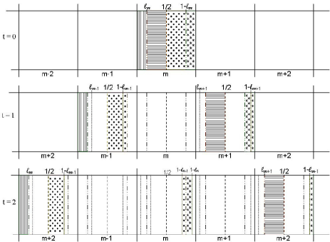
It is also time reversal invariant (TRI), i.e. there exists an involution $i$ such that $iS=S^{-1}i$, e.g. the one defined by $i(x,m)=(1-x,m)$ will do. The action of $S$ is illustrated by Fig.1, for an initial condition concentrated and uniform in $\widehat{M}_{m}$.

Figure 1: Two time steps of the slicer map, for initial conditions in cell $\widehat{M}_{m}$. For the sake of the figure a vertical coordinate has been added.

For every $\alpha>0$, let us introduce the family of slicers:

$$L_{\alpha}=\left\{\Big{(}\ell_{j}(\alpha),1-\ell_{j}(\alpha)\Big{)}:\ell_{j}(\alpha)=\frac{1}{\left(\left|j\right|+2^{1/\alpha}\right)^{\alpha}},\,j\in\mathbb{Z}\right\}$$ (8)

Then, the slicer map is denoted by $S_{\alpha}$ if all slicers of Eq.(6) belong to $L_{\alpha}$: $\ell_{m}=\ell_{m}(\alpha)$. Obviously, for every $\alpha>0$, $S_{\alpha}$ preserves $\hat{\mu}$ and is not chaotic (its Lyaponuv exponents vanish). Indeed, different points in $\widehat{M}$ neither converge nor diverge from each other in time, except when separated by a slicer, in which case their distance jumps. But like for two particles in a polygonal billiard, one of which hits a corner of the polygon while the other continues its free flight [2], the separation points constitute a set of zero $\hat{\mu}$ measure, hence they do not suffice to produce positive Lyapunov exponents.

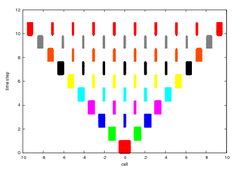
The transport properties of the Slicer Dynamics will be examined by taking an ensemble of points $\widehat{E}_{0}$ in the central cell $\widehat{M}_{0}=M\times\left\{0\right\}$ and studying the way $S_{\alpha}$ spreads them in $\widehat{M}$. One finds that in $n$ time steps the points of $\widehat{E}_{0}$ reach $\widehat{M}_{n}$ and $\widehat{M}_{-n}$, and that the cells occupied at time $n$ have odd index if $n$ is odd, and have even index if $n$ is even, as illustrated in Fig. 2 for a given $\alpha$.

Figure 2: Ten time steps of $S_{\alpha}$, with $\alpha=1/3$, for $N=10^{4}$ points initially uniformly distributed in $\widehat{M}_{0}$. The direction of time is the vertical axis. For the sake of the figure, an extra inactive vertical coordinate has been added.

More precisely, taking

$$P_{n}=\{j\in\mathbb{Z}:j\ \mbox{is even and\ }|j|\leq n\},\quad D_{n}=\{j\in\mathbb{Z}:j\ \mbox{is odd and\ }|j|\leq n\},$$ (9)

we have

$$S_{\alpha}^{n}~{}\widehat{M}_{0}=\bigcup_{j\in P_{n}}\big{(}R_{j}\times\{j\}\big{)}\quad\mbox{if~{}}n\mbox{~{}is even}~{},\qquad S_{\alpha}^{n}~{}\widehat{M}_{0}=\bigcup_{j\in D_{n}}\big{(}R_{j}\times\{j\}\big{)},\quad\mbox{if~{}}n\mbox{~{} is odd}$$ (10)

where $R_{j}\times\{j\}\subset\widehat{M}_{j}$, and $R_{j}\subset M$ is an interval or a union of intervals if $\widehat{E}_{0}=\widehat{M}_{0}$.

Let $d\nu_{0}:=\hat{\rho}_{0}(\widehat{X})d\hat{\mu}$ be a probability measure on $\widehat{M}$ with density

$$\hat{\rho}_{0}\left(\widehat{X}\right)=\left\{\begin{array}[]{rl}1,&\mbox{if }\widehat{X}\in M_{0}\\ 0,&\mbox{otherwise}\end{array}\right.$$ (11)

This measure evolves under the action of $S_{\alpha}$ describing the transport of an ensemble of points initially uniformly distributed in $\widehat{M}_{0}$. For simplicity, in the following we will always adopt this initial condition, which mimics the $\delta$-function initial condition common in standard diffusion theory; if the initial condition were confined within $\widehat{M}_{m}$ with $m\neq 0$, nothing would change in practice.

Requiring the conservation of probability, the evolution $\nu_{n}$ of $\nu_{0}$ at time $n$ is given by $\nu_{n}(\widehat{R})=\nu_{0}(S^{-n}_{\alpha}\widehat{R})$, for every measurable $\widehat{R}\subset\widehat{M}$. Its density is given by:

$$\hat{\rho}_{n}(\widehat{X})=\left\{\begin{array}[]{rl}1,&\mbox{if }\widehat{X}\in S_{\alpha}^{n}\widehat{M}_{0}~{}~{}~{}\left(\mbox{or, equivalently, if ~{}}S_{\alpha}^{-n}\widehat{X}\in\widehat{M}_{0}\right)\\ 0,&\mbox{otherwise}.\end{array}\right.$$ (12)

Consider the sets

$$\widehat{R}_{j}:=S^{n}_{\alpha}(\widehat{M_{0}})\cap{\widehat{M}_{j}},\quad j=-n,\ldots,n,$$ (13)

which constitute the total phase space volume occupied at time $n$ in cell ${\widehat{M}_{j}}$. Their measure

$$A_{j}:=\hat{\mu}(\widehat{R_{j}})=\lambda(\pi_{M}(\widehat{R_{j}}))\delta_{\mathbb{Z}}(j)=\lambda(\pi_{M}(\widehat{R_{j}})),$$ (14)

equals the probability $\nu_{n}(\widehat{M}_{j})$ of cell $j$ at time $n$: as $\hat{\mu}$ is invariant and $S_{\alpha}$ invertible, we have

$$A_{j}=\hat{\mu}(\widehat{R}_{j})=\hat{\mu}(S^{-n}_{\alpha}(\widehat{R}_{j}))=\hat{\mu}(\widehat{M_{0}}\cap S^{-n}_{\alpha}(\widehat{M_{j}}))=\nu_{0}(S^{-n}_{\alpha}(\widehat{M_{j}}))=\nu_{n}({\widehat{M}_{j}})~{},$$

and $\sum_{j=-n}^{n}A_{j}=\hat{\mu}(\cup_{j=-n}^{n}S^{n}_{\alpha}(\widehat{M}_{0})\cap{\widehat{M}_{j}})=\widehat{\mu}(S^{n}_{\alpha}(\widehat{M_{0}}))=\hat{\mu}(\widehat{M_{0}})=1$. Indeed, $S^{n}_{\alpha}(\widehat{M_{0}})\cap{\widehat{M}_{j}}=\emptyset$ for $|j|>n$ and $\cup_{j=-\infty}^{\infty}{\widehat{M}_{j}}=\widehat{M}$. In other words, the $A_{j}$’s define a probability distribution which coincides with $\nu_{n}(\pi_{\mathbb{Z}}^{-1})$ and, thus, is a marginal probability distribution of $\nu_{n}$. Starting from the “microscopic” distribution $\nu_{n}$ on $\widehat{M}$, we can now introduce its coarse grained version $\rho_{n}^{G}$, as the following measure on the integer numbers $\mathbb{Z}$:

Definition 2.1.

For every time $n\in\mathbb{N}$, the Coarse Grained Distribution is defined by

$$\rho^{G}_{n}(j)=\left\{\begin{array}[]{rl}A_{j}&\mbox{if }j\in\{-n,\ldots,n\},\\ 0&\mbox{\rm otherwise.}\end{array}\right.$$ (15)

$A_{-n}$ and $A_{n}$ are called traveling areas; $A_{j}$ is called sub-traveling area if $|j|<n$.

Remark 1.

From the definition of $S_{\alpha}$ and the initial condition (11), we have $A_{j}=A_{-j}$ for all $j\in\mathbb{Z}$. Thus, $\rho^{G}_{n}(j)$ is even, $\rho^{G}_{n}(j)=\rho^{G}_{n}(-j)$, and all its odd moments vanish.

The Coarse Grained Distribution will be used to describe the transport properties of the coarse grained trajectories $\{\pi_{\mathbb{Z}}(S^{n}_{\alpha}(\widehat{X}_{0}))\}_{n\in\mathbb{N}}\subset\mathbb{Z}$, with $\widehat{X}_{0}\in\widehat{M}_{0}$. This way, $\rho_{n}^{G}$ becomes the discrete analogous of the mass concentration $c(x,t)$ of Eqs.(1) and (2), and we can introduce the discrete versions of Eqs.(4) and (5) as follows:

Definition 2.2.

The mean square displacement induced at time $n$ by $S_{\alpha}$ is the second moment

$$\langle\Delta\hat{X}^{2}_{n}\rangle:=\sum_{j=-n}^{n}A_{j}j^{2}$$ (16)

of $\rho_{n}^{G}$, where $j$ is the distance travelled by a point in $\widehat{M}_{j}$ at time $n$. Then, for $\gamma\in[0,2]$ let

$$T_{\alpha}(\gamma):=\lim_{n\rightarrow\infty}\frac{\langle\Delta\hat{X}^{2}_{n}\rangle}{n^{\gamma}}~{}.$$ (17)

If $T_{\alpha}(\gamma^{t})\in(0,\infty)$ for $\gamma^{t}\in[0,2]$, $\gamma^{t}$ is called the transport exponent of the Slicer Dynamics, and $T_{\alpha}(\gamma^{t})$ the generalized diffusion coefficient.

Remark 2.

The mean displacement $\langle\Delta\hat{X}_{n}\rangle:=\sum_{j=-n}^{n}A_{j}j$ vanishes at all $n$, hence there is no drift in the Slicer Dynamics.

Note that $A_{j}$ equals the width of the interval $R_{j}$, which is determined by the position of the slicers in the $j$-th cell, once $\alpha$ is given. Therefore, $A_{j}$ can be computed directly from Eq.(8). For the traveling areas we have

$$A_{n}=\ell_{n-1}=\left(\frac{1}{|n|-1+2^{1/\alpha}}\right)^{\alpha}=A_{-n}$$ (18)

while for the non vanishing sub-traveling areas we have:

$$A_{j}=\ell_{\left|j\right|-1}-\ell_{\left|j\right|+1}=\frac{1}{\left(\left|j\right|-1+2^{1/\alpha}\right)^{\alpha}}-\frac{1}{\left(\left|j\right|+1+2^{1/\alpha}\right)^{\alpha}}~{},$$ (19)

For even $n>2$, this implies

$${\rho}^{G}_{n}(j)=\left\{\begin{array}[]{rl}2(\ell_{0}-\ell_{1})~{},&\ \ \mbox{for }j=0\\ \ell_{\left|2k-1\right|}-\ell_{\left|2k+1\right|}~{},&\ \ \mbox{for }|j|=2k,\,\ k=1,\ldots,\frac{n-2}{2}\\ \ell_{\left|n-1\right|}~{},&\ \ \mbox{for }|j|=n\\ 0~{},&\ \ \mbox{elsewhere}\end{array}\right.$$ (20)

while for odd $n>3$, it implies:

$${\rho}^{G}_{n}(j)=\left\{\begin{array}[]{rl}\ell_{\left|2k\right|}-\ell_{\left|2k+2\right|}~{},&\ \ \mbox{for }|j|=2k+1,\ k=0,\ldots,\frac{n-3}{2}\\ \ell_{\left|n-1\right|}~{},&\ \ \mbox{for }|j|=n\\ \ 0~{},&\ \ \mbox{elsewhere}\end{array}\right.$$ (21)

Remark 3.

Using Eq.(8) in Eqs.(21) and (20) for large $n$, one obtains that the tail of the distribution (large $j$) goes (independently of the parity of $n$) like: ${\rho}^{G}_{n}(j)\sim{\displaystyle 2\alpha}/{\displaystyle|j|^{\alpha+1}}{\mathbb{I}}_{\{|j|<n\}}$, i.e. ${\rho}^{G}_{n}$ has heavy tails. In particular, for $\alpha=1/2$, ${\rho}^{G}_{n}$ has tails falling like those of the Lévy distribution, $|j|^{-3/2}$. For $j=\pm n$ the probability is much larger: ${\rho}^{G}_{n}(n)\sim{\displaystyle 1}/{\displaystyle|n|^{\alpha}}$.

Now we may state the following:

Proposition 2.1.

Given $\alpha\in\left(0,2\right)$ and the uniform initial distribution in $\widehat{M}_{0}$, we have:

$$T_{\alpha}(\gamma)=\left\{\begin{array}[]{rl}+\infty&\mbox{if }0\leq\gamma<2-\alpha\\ \frac{4}{2-\alpha}&\mbox{if }\gamma=2-\alpha\\ 0&\mbox{if }2-\alpha<\gamma\leq 2\end{array}\right.$$ (22)

hence the transport exponent $\gamma^{t}$ takes the value $2-\alpha$.

Proof.

For the symmetry of $\rho^{G}_{n}$, it suffices to consider the cells $\widehat{M}_{j}$ with $j\in\mathbb{N}$:

$$T_{\alpha}(\gamma)=2\lim_{n\to\infty}\frac{1}{n^{\gamma}}\sum_{j=0}^{n}A_{j}j^{2}=2\lim_{n\to\infty}\frac{1}{n^{\gamma}}\left(\sum_{j=0}^{n-1}A_{j}j^{2}+A_{n}n^{2}\right).$$ (23)

Let us focus on the sub-travelling areas first. Lemma 2.2 proved below states that:

$$\lim_{n\to\infty}\frac{1}{n^{\gamma}}\sum_{j=0}^{n-1}A_{j}j^{2}=\left\{\begin{array}[]{rl}\infty&\ \ \mbox{if }0\leq\gamma<2-\alpha\\ \dfrac{\alpha}{2-\alpha}&\ \ \mbox{if }\gamma=2-\alpha\\ 0&\ \ \mbox{if }2-\alpha<\gamma\leq 2\end{array}\right.$$ (24)

Because of Eq.(18), the travelling area yields:

$$\lim_{n\to\infty}\frac{n^{2}}{(n+2^{1/\alpha}-1)^{\alpha}}\cdot\frac{1}{n^{\gamma}}=\left\{\begin{array}[]{rl}\infty&\mbox{if }0\leq\gamma<2-\alpha\\ 1&\mbox{if }\gamma=2-\alpha\\ 0&\mbox{if }2-\alpha<\gamma\leq 2\end{array}\right.$$ (25)

Thus, $T_{\alpha}(\gamma)$ is given by:

$$T_{\alpha}(\gamma)=\left\{\begin{array}[]{rl}\infty&\mbox{if }0\leq\gamma<2-\alpha\\ \frac{4}{2-\alpha}&\mbox{if }\gamma=2-\alpha\\ 0&\mbox{if }2-\alpha<\gamma\leq 2\end{array}\right.$$ (26)

As $\gamma^{t}$ is the value $\gamma$ for which $T_{\alpha}(\gamma)$ is finite, we have $\gamma^{t}=2-\alpha$. ∎

The proof of Proposition (2.1) depends on the next lemma.

Lemma 2.2.

Given $\alpha\in(0,2)$, let $Q_{n}:=\sum_{j=0}^{n-1}A_{j}j^{2}$ be the contribution to the mean square displacement of the sub-travelling areas. Then:

$$\lim_{n\to\infty}\frac{Q_{n}}{n^{\gamma}}=\left\{\begin{array}[]{rl}\infty&\ \ \mbox{if }0\leq\gamma<2-\alpha\\ \frac{\alpha}{2-\alpha}&\ \ \mbox{if }\gamma=2-\alpha\\ 0&\ \ \mbox{if }2-\alpha<\gamma\leq 2\end{array}\right.$$ (27)

Proof.

The series $Q_{n}$ assumes a different form depending on wheter $n$ is even or odd. If it is even and larger than $2$,

$$Q_{n}=\sum_{j=0,j\in P_{n}}^{n-1}A_{j}j^{2}=4\sum_{j=1}^{\frac{n}{2}-1}\left[\frac{1}{\left(2j+2^{1/\alpha}-1\right)^{\alpha}}-\frac{1}{\left(2j+2^{1/\alpha}+1\right)^{\alpha}}\right]\;j^{2}$$ (28)

This sum has a telescopic structure that allows us to rewrite it as follows:

$$Q_{n}=4~{}\sum_{j=1}^{\frac{n}{2}-1}\frac{2j-1}{\left(2j-1+2^{1/\alpha}\right)^{\alpha}}-\frac{\left(n-2\right)^{2}}{\left(n-1+2^{1/\alpha}\right)^{\alpha}}.$$ (29)

Let $R_{n}$ be the first term of $Q_{n}$. Introducing $f(j):=\frac{2j-1}{\left(2j-1+2^{1/\alpha}\right)^{\alpha}}$ we can write:

$$R_{n}=4~{}\sum_{j=1}^{\frac{n}{2}-1}\frac{2j-1}{\left(2j-1+2^{1/\alpha}\right)^{\alpha}}=4~{}\sum_{j=1}^{\frac{n}{2}-1}f(j).$$ (30)

The derivative

$$f^{\prime}(j)=\frac{2\left[2(1-\alpha)j+2^{1/\alpha}+\alpha-1\right]}{(2j+2^{1/\alpha}-1)^{\alpha+1}}$$ (31)

shows that $f$ is increasing for $0<\alpha\leq 1$, while for $1<\alpha<2$, $f$ grows for $j<j(\alpha)$ and decreases for $j>j(\alpha)$, with $j(\alpha)=(1-\alpha-2^{1/\alpha})/2(1-\alpha)$. For $0<\alpha\leq 1$, $f$ is strictly increasing, hence:

$$\int_{0}^{\frac{n}{2}-1}f(x)dx\leq\sum_{j=1}^{\frac{n}{2}-1}f(j)\leq\int_{1}^{\frac{n}{2}}f(x)dx.$$ (32)

We have to distinguish two cases: $\alpha<1$ and $\alpha=1$. In the first case we have:

$$\int_{0}^{\frac{n}{2}-1}f(x)dx = \frac{1}{2}\left[\frac{(n-3+2^{1/\alpha})^{2-\alpha}}{2-\alpha}-2^{1/\alpha}\cdot\frac{(n-3+2^{1/\alpha})^{1-\alpha}}{1-\alpha}\right.+$$ (33)

$$+ \left.\left(2^{1/\alpha}-1\right)^{1-\alpha}\cdot\frac{2^{1/\alpha}-\alpha+1}{(2-\alpha)(1-\alpha)}\right]$$

and

$$\int_{1}^{\frac{n}{2}}f(x)dx = \frac{1}{2}\left[\frac{(n-1+2^{1/\alpha})^{2-\alpha}}{2-\alpha}-2^{1/\alpha}\cdot\frac{(n-1+2^{1/\alpha})^{1-\alpha}}{1-\alpha}\right.+$$ (34)

$$+ \left.(2^{1/\alpha}+1)^{1-\alpha}\cdot\frac{(2^{1/\alpha}+\alpha-1)}{(2-\alpha)(1-\alpha)}\right]$$

therefore taking the $n\rightarrow\infty$ limit we have:

$$\lim_{n\to\infty}\frac{1}{n^{\gamma}}\int_{0}^{\frac{n}{2}-1}f(x)dx=\left\{\begin{array}[]{rl}\infty&\mbox{if }0\leq\gamma<2-\alpha\\ \frac{1}{2(2-\alpha)}&\mbox{if }\gamma=2-\alpha\\ 0&\mbox{if }2-\alpha<\gamma\leq 2\end{array}\right.$$ (35)

and

$$\lim_{n\to\infty}\frac{1}{n^{\gamma}}\int_{1}^{\frac{n}{2}}f(x)dx=\left\{\begin{array}[]{rl}\infty&\mbox{if }0\leq\gamma<2-\alpha\\ \frac{1}{2(2-\alpha)}&\mbox{if }\gamma=2-\alpha\\ 0&\mbox{if }2-\alpha<\gamma\leq 2\end{array}\right.$$ (36)

For $\alpha=1$ the two integrals differ, but the bounding limits coincide, therefore, one obtains:

$$\lim_{n\to\infty}\frac{R_{n}}{n^{\gamma}}=\lim_{n\to\infty}\frac{4}{n^{\gamma}}\sum_{j=1}^{\frac{n}{2}-1}f(j)=\left\{\begin{array}[]{rl}\infty&\mbox{if }0\leq\gamma<2-\alpha\\ \dfrac{2}{2-\alpha}&\mbox{if }\gamma=2-\alpha\\ 0&\mbox{if }2-\alpha<\gamma\leq 2\end{array}\right.$$ (37)

If $1<\alpha<2$, $f$ deacreses for $j>j(\alpha)$ hence, introducing $\bar{j}_{\alpha}=\left\lfloor j(\alpha)\right\rfloor$, where $\left\lfloor x\right\rfloor$ is the integer part of $x$, $R_{n}$ can be expressed as:

$$R_{n}=4\left(\sum_{j=1}^{\bar{j}_{\alpha}}f(j)+\sum_{j=\bar{j}_{\alpha}+1}^{\frac{n}{2}-1}f(j)\right)$$ (38)

Dividing by $n^{\gamma}$ and taking the $n\to\infty$ limit, the first term vanishes for all $\gamma>0$, while the second term can be treated as above, to obtain the same as Eq.(37). Recalling Eq.(29), this eventually implies (27). For odd $n$, one proceeds similarly. ∎

Remark 4.

For $\alpha\in(0,2)$, Proposition (2.1) states that the mean square displacement goes like $\langle\Delta\hat{X}^{2}_{n}\rangle\sim n^{2-\alpha}$. Thus, the trivial map $S_{\alpha}$ enjoys all possible regimes of standard and anomalous diffusion, as $\alpha$ varies in $(0,2)$.

The next proposition concerns the transport behavior for $\alpha=2$.

Proposition 2.3.

Given $\alpha=2$ and the uniform initial distribution in $\widehat{M}_{0}$, we have:

$$T_{2}(\gamma)=\left\{\begin{array}[]{rl}+\infty&\mbox{if }\ \ \gamma=0\\ 0&\mbox{if }\ \ 0<\gamma\leq 2\end{array}\right.$$ (39)

More precisely, the dynamics is “logarithmically diffusive”, i.e.

$$\langle\Delta\hat{X}^{2}_{n}\rangle\sim\log n~{},~{}~{}\mbox{asymptotically in $n$.}$$

Proof.

Repeat the previous reasoning with $\alpha=2$ and correspondingly different integrals. ∎

We can now state the following theorem which gives the asymptotic behavior of the moments of the displacement $\Delta\hat{X}^{p}_{n}$, i.e. of the moments of $\rho^{G}_{n}$:

$$\langle\Delta\hat{X}^{p}_{n}\rangle=\sum_{j=-n}^{n}A_{j}j^{p}$$ (40)

Theorem 2.4.

For $\alpha\in\left(0,2\right]$ the moments $\langle\Delta\hat{X}^{p}_{n}\rangle$ with $p>2$ even and initial condition uniform in $\widehat{M}_{0}$ have the following asymptotic beahvior:

$$\langle\Delta\hat{X}^{p}_{n}\rangle\sim n^{p-\alpha}~{},$$

while the odd moments ($p=1,3,...$) vanish.

Proof.

We want to compute the following limit:

$$L(\alpha,p):=\lim_{n\to\infty}\frac{1}{n^{\gamma}}{\langle\Delta\hat{X}^{p}_{n}\rangle}=\lim_{n\to\infty}\ \frac{1}{n^{\gamma}}\sum_{j=-n}^{n}A_{j}j^{p}.$$ (41)

As observed in Remark 2, the symmetry of $\rho^{G}_{n}$ leads the sums with odd $p$ to vanish. For the even moments it suffices to consider the positive $j$’s:

$$L(\alpha,p)=\lim_{n\to\infty}\frac{2}{n^{\gamma}}\left(\sum_{j=0}^{n-1}A_{j}j^{p}+A_{n}n^{p}\right).$$ (42)

In next Lemma 2.5 it is shown that:

$$\lim_{n\to\infty}\frac{1}{n^{\gamma}}\sum_{j=0}^{n-1}A_{j}j^{p}=\left\{\begin{array}[]{rl}\infty&\ \ \mbox{if }0\leq\gamma<p-\alpha\\ \dfrac{\alpha}{p-\alpha}>0&\ \ \mbox{if }\gamma=p-\alpha\\ 0&\ \ \mbox{if }\gamma>p-\alpha\end{array}\right.$$ (43)

while for the travelling area (18) we have:

$$\lim_{n\to\infty}A_{n}n^{p}=\lim_{n\to\infty}\frac{n^{p}}{(n+2^{1/\alpha}-1)^{\alpha}}\cdot\frac{1}{n^{\gamma}}=\left\{\begin{array}[]{rl}\infty&\mbox{if }0\leq\gamma<p-\alpha\\ 1&\mbox{if }\gamma=p-\alpha\\ 0&\mbox{if }\gamma>p-\alpha.\end{array}\right.$$ (44)

Therefore, we conclude that

$$L(\alpha,p)=\left\{\begin{array}[]{rl}\infty&\mbox{if }0\leq\gamma<p-\alpha\\ \dfrac{p}{p-\alpha}&\mbox{if }\gamma=p-\alpha\\ 0&\mbox{if }\gamma>p-\alpha\end{array}\right.$$ (45)

so that the large $n$ behavior of the even moments is given by $\langle\Delta\hat{X}^{p}_{n}\rangle\sim n^{p-\alpha}$. ∎

Lemma 2.5.

For the sub-travelling areas and any $\alpha\in(0,2]$, the following holds:

$$\lim_{n\to\infty}\frac{1}{n^{\gamma}}\sum_{j=0}^{n-1}A_{j}j^{p}=\left\{\begin{array}[]{rl}\infty&\ \ \mbox{if }0\leq\gamma<p-\alpha\\ \dfrac{\alpha}{p-\alpha}&\ \ \mbox{if }\gamma=p-\alpha\\ 0&\ \ \mbox{if }\gamma>p-\alpha.\end{array}\right.$$ (46)

Proof.

Let us begin with even $n$. Defining $\mathcal{P}_{n}$ as

$$\mathcal{P}_{n}:=\sum_{j=0,j\in P_{n}}^{n-1}A_{j}j^{p}=2^{p}\sum_{j=1}^{\frac{n}{2}-1}\left[\frac{1}{\left(2j+2^{1/\alpha}-1\right)^{\alpha}}-\frac{1}{\left(2j+2^{1/\alpha}+1\right)^{\alpha}}\right]\;j^{p}$$ (47)

induction leads to:

$$\mathcal{P}_{n}=2^{p}\cdot\sum_{j=0}^{\frac{n}{2}-2}\frac{(j+1)^{p}-j^{p}}{\left(2j+1+2^{1/\alpha}\right)^{\alpha}}-\frac{\left(n-2\right)^{p}}{\left(n-1+2^{1/\alpha}\right)^{\alpha}}=R_{n}-\frac{\left(n-2\right)^{p}}{\left(n-1+2^{1/\alpha}\right)^{\alpha}}~{},$$ (48)

which defines $R_{n}$ in terms of addends of the form:

$$f(j)=\frac{(j+1)^{p}-j^{p}}{(2j+1+2^{1/\alpha})^{\alpha}}=\sum_{k=1}^{p}\binom{p}{k}\frac{j^{p-k}}{(2j+1+2^{1/\alpha})^{\alpha}}$$ (49)

with derivative given by:

$$f^{\prime}(j)=\sum_{k=1}^{p}\binom{p}{k}\frac{\left[2(p-k-\alpha)j+(p-k)(1+2^{1/\alpha})\right]}{(2j+1+2^{1/\alpha})^{\alpha+1}}j^{p-k-1}=\sum_{k=1}^{p}f_{k}(j)~{}.$$ (50)

where

$$f_{k}(j)=\binom{p}{k}\frac{\left[2(p-k-\alpha)j+(p-k)(1+2^{1/\alpha})\right]}{(2j+1+2^{1/\alpha})^{\alpha+1}}j^{p-k-1}$$ (51)

For $0<\alpha\leq 1$ and all $j>0$, we have $f_{k}(j)>0$ for $k=1,\ldots,p-1$, while $f_{p}(j)<0$. Because $|f_{p}(j)|<f_{1}(j)$, $f^{\prime}$ is positive and $f$ increases for all $j>0$. For $1<\alpha\leq 2$ and $p=3$, one has $f(j)=(3j^{2}+3j+1)/(2j+1+2^{1/\alpha})^{\alpha}$, which is increasing for $j>0$, while for $p\geq 4$ one obtains $f_{k}(j)>0$ for $k=1,\ldots,p-2$, and $f_{p-1}(j),f_{p}(j)<0$. Because $|f_{p-1}(j)+f_{p}(j)|<f_{1}(j)+f_{2}(j)$, $f(j)$ is increasing for $j>0$, even for $1<\alpha\leq 2$.

Therefore, we can bound our sum from above and below as follows:

$$\int_{0}^{\frac{n}{2}-2}f(x)dx<\sum_{j=0}^{\frac{n}{2}-2}f(j)<\int_{1}^{\frac{n}{2}-1}f(x)dx.$$ (52)

for all $\alpha\in(0,2]$. Passing to the limit as previously done, we eventually obtain:

$$\lim_{n\to\infty}\frac{R_{n}}{n^{\gamma}}=\left\{\begin{array}[]{rl}\infty&\mbox{if }0\leq\gamma<p-\alpha\\ \dfrac{p}{2^{p}(p-\alpha)}&\mbox{if }\gamma=p-\alpha\\ 0&\mbox{if }\gamma>p-\alpha\end{array}\right.\quad\lim_{n\to\infty}\frac{\mathcal{P}_{n}}{n^{\gamma}}=\left\{\begin{array}[]{rl}\infty&\mbox{if }0\leq\gamma<p-\alpha\\ \dfrac{\alpha}{p-\alpha}&\mbox{if }\gamma=p-\alpha\\ 0&\mbox{if }\gamma>p-\alpha\end{array}\right.$$ (53)

for all $\alpha\in(0,2]$. If $n$ is odd, one proceeds similarly to obtain the same result.

∎

3 Examples

In this section, we illustrate numerically the transport produced by the Slicer Map $S_{\alpha}$ for two different values of $\alpha$. The initial condition uniform in $\widehat{M}_{0}$ is approximated by $N$ points uniformly distributed at random on $\widehat{M}_{0}$, so that the mean square displacement is approximated by:

$$\langle\Delta\widehat{X}_{n}^{2}\rangle\approx\frac{1}{N}\sum_{i=1}^{N}\ d_{\widehat{M}}\left(S_{\alpha}^{n}\widehat{X}_{0}(i),\widehat{X}_{0}(i)\right)^{2}$$ (54)

where $\widehat{X}_{0}(i)$ is the $i$-th point initial position and $d_{\widehat{M}}(\widehat{X},\widehat{Y})=k$ if $\widehat{X}\in\widehat{M}_{m}$ and $\widehat{Y}\in\widehat{M}_{m\pm k}$.

Example 1.

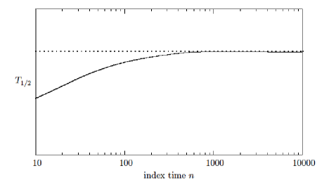
$\alpha=1/2$: in this case $\ell_{j}(1/2)={1}/\big{(}\left|j\right|+4\big{)}^{1/2}$, and the asymptotic behavior is $\left\langle\Delta\widehat{X}^{2}_{n}\right\rangle\sim n^{{3}/{2}}$, cf. Remark (4), which means that $S_{1/2}$ is super-diffusive with $\gamma^{t}=3/2$, and generalized diffusion coefficient $T_{1/2}={8}/{3}$, as illustrated by Fig.3. Moreover, for $p>2$ Theorem 2.4 implies that:

$$\langle\Delta\widehat{X}^{p}_{n}\rangle\sim n^{p-{1}/{2}}$$ (55)

For the coarse grained distribution, cf. (20) and (21), even $n$ yields:

$$\rho^{G}_{n}\left(m\right)=\left\{\begin{array}[]{rl}\frac{1}{2}-\frac{1}{\sqrt{5}},&\ \ \mbox{for }m=0\\ \frac{1}{\sqrt{2k+3}}-\frac{1}{\sqrt{2k+5}},&\ \ \mbox{for }m=2k,\ k=2,\ldots,\frac{n-2}{2}\\ \frac{1}{\sqrt{n+3}}&\ \ \mbox{for }m=n\\ 0,&\ \ \mbox{otherwise}\end{array}\right.$$ (56)

while odd $n$ yields:

$$\rho^{G}_{n}\left(m\right)=\left\{\begin{array}[]{rl}\frac{1}{\sqrt{2k+4}}-\frac{1}{\sqrt{2k+6}},&\ \ \mbox{for }m=2k+1,\ k=2,\ldots,\frac{n-3}{2}\\ \frac{1}{\sqrt{n+3}}&\ \ \mbox{for }m=n\\ 0,&\ \ \mbox{otherwise}\end{array}\right.$$ (57)

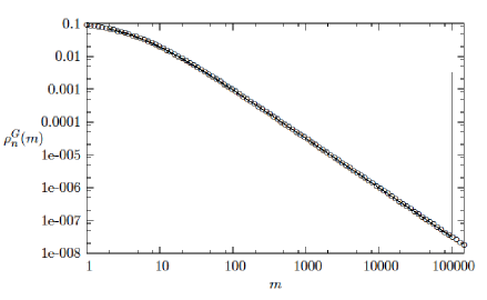
Figure 4 shows the numerically computed marginal probability distribution function $\rho^{G}_{n}(m)$ at a fixed even $n$, for $m>0$, including the last value $\rho^{G}_{n}(n)$, which is much larger than the values for $m$ close to $n$ (the negative branch of the distribution can be recovered by symmetriy). Because asymptotically $\rho^{G}_{n}$ goes like:

$$\rho^{\alpha}_{n}(m)=\left\{\begin{array}[]{rr}\frac{\displaystyle C_{\alpha}}{\displaystyle(m+2^{1/\alpha})^{\alpha+1}}~{},&m<n,\\ 0~{},&m>n,\end{array}\right.$$ (58)

where $C_{\alpha}$ is a normalization constant, Figure 4 compares the numerical values of $\rho^{G}_{n}$ with $\rho^{1/2}_{n}(m)$, with $C_{1/2}=1$. Apart from $\rho^{G}_{n}(n)$, $\rho^{1/2}_{n}$ perfectly fits the real distribution.

Figure 3: Behavior of the numerically estimated coefficient $T_{1/2}$ (continuous line) for $n=10^{4}$ and for a choice of $N=10^{3}$ points compared with its theoretical value $\frac{8}{3}$ (dotted line) obtained from (22).

Figure 4: Log-log plot of the marginal probability distribution function $\rho_{n}^{G}(m)$ (continuous line) for map $S_{1/2}$ compared with $\rho^{1/2}(x)=C_{1/2}/(x+4)^{3/2}$ (circles) at fixed $n=10^{5}$. The peak at $m=n$ is produced by the traveling area.

Example 2.

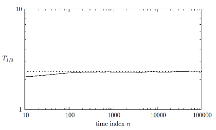
$\alpha=1/3$: this is the case illustrated by Fig.(2), for which we have $\ell_{j}(1/3)={1}/{\left(\left|j\right|+8\right)^{1/3}}$, and asymptotic behavior given by $\langle\Delta\widehat{X}^{2}_{n}\rangle\sim n^{{5}/{3}}$. This means that $S_{1/3}$ is super-diffusive with $\gamma^{t}=5/3$, and generalized diffusion coefficient $T_{1/3}={12}/{5}$ (cf. Fig. 5). From Theorem 2.4, the moments of $S_{1/3}$ higher than the second have the following behavior:

$$\langle\Delta\widehat{X}^{p}_{n}\rangle\sim n^{p-{1}/{3}}$$ (59)

The coarse grained distribution, see (20) and (21), for even $n$ reads:

$$\rho^{G}_{n}\left(m\right)=\left\{\begin{array}[]{rl}\frac{1}{2}-\frac{1}{\sqrt[3]{9}},&\ \ \mbox{for }m=0\\ \frac{1}{\sqrt[3]{2k+7}}-\frac{1}{\sqrt[3]{2k+9}},&\ \ \mbox{for }m=2k,\ k=2,\ldots,\frac{n-2}{2}\\ \frac{1}{\sqrt[3]{n+7}}&\ \ \mbox{for }m=n\\ 0,&\ \ \mbox{otherwise}\end{array}\right.$$ (60)

while for odd $n$ we have:

$$\rho^{G}_{n}\left(m\right)=\left\{\begin{array}[]{rl}\frac{1}{\sqrt[3]{2k+8}}-\frac{1}{\sqrt[3]{2k+10}},&\ \ \mbox{for }m=2k+1,\ k=2,\ldots,\frac{n-3}{2},\\ \frac{1}{\sqrt[3]{n+7}}&\ \ \mbox{for }m=n\\ 0,&\ \ \mbox{otherwise}\end{array}\right.$$ (61)

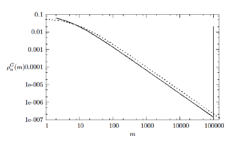
Figure 6 compares the marginal probability distribution function $\rho^{G}_{n}(m)$ with $\rho^{1/3}_{n}$ given by (58). Apart from the value $\rho^{G}_{n}(n)$, the asymptotic behaviours coincide once $C_{1/3}$ is fixed.

Figure 5: Numerical estimate of $T_{1/3}$ (continuous line) for $n=10^{5}$ time steps and $N=10^{5}$ points, compared with its theoretical value ${12}/{5}$ (dotted line) obtained from (22).

Figure 6: Log-log pot of the marginal probability distribution function $\rho_{n}^{G}(m)$ for map $S_{1/3}$ and even $m$ (continuous line), compared with $\rho^{1/3}_{n}$ (dotted line) at fixed time $n=10^{5}$. A part from the values at $m=n$, where $\rho_{n}^{G}$ has a spike due to the travelling area, the asymptotic behaviours coincide once the normalization constant of $\rho^{1/3}_{t}$ is adjusted.

4 Slicer Map and Lévy Walks

4.1 Lévy Walks in quenched disordered media

In this section we compare the Slicer transport properties with those of the Lévy walks in quenched disordered media of Ref.[16], in which a one-dimensional sequence of scatterers obeys a Lévy type distribution, with probability density for two consecutive scatterers to be at distance $r$ given by:

$$\lambda(r)\equiv\beta r_{0}^{\beta}\frac{1}{r^{\beta+1}},\ \ r\in\left[r_{0},+\infty\right)$$ (62)

where $\beta>0$ and $r_{0}$ is a cutoff fixing the characteristic length scale of the system. Then, a walker moves ballistically (at constant velocity $v$) until it reaches one of the scatterers, from which it is either transmitted or reflected with probability $1/2$. The authors of [16] derive an analytic expression for the asymptotic behavior of the mean square displacement $\langle r^{2}(t)\rangle$ when averaged over the scattering points. At first they introduce the most general scaling hypothesis for the probability distribution $P(r,t)$ for the walker to be in position $r$ at time $t$:

$$P(r,t)=l^{-1}(t)f\left(\frac{r}{l(t)}\right)+g(r,t)$$ (63)

where $l(t)$ is the characteristic length of $P$ and the following is assumed:

$$\lim_{t\to+\infty}\int_{0}^{vt}\left|P(r,t)-l^{-1}(t)f\left({r}/{l(t)}\right)\right|dr=0~{};\quad\lim_{t\to+\infty}\int\left|g(r,t)\right|dr=0~{}.$$ (64)

The first integral stops at $vt$ because the random walker covers at most a distance $vt$ in a time $t$. For the same reason, the expression of the mean square displacement reads:

$$\langle r^{2}(t)\rangle=\int_{0}^{vt}l^{-1}(t)f\left({r}/{l(t)}\right)r^{2}dr+\int_{0}^{vt}g(r,t)r^{2}dr~{}.$$ (65)

Exploiting the equivalence with an electric problem [20], the calculation of the number $N(t)$ of scattering sites visited by the walker in a time $t$ takes the form [16]:

$$N(t)\sim\left\{\begin{array}[]{rl}t^{\frac{\beta}{1+\beta}}~{},&\ \mbox{if }0<\beta<1\\ t^{1/2}~{},&\ \mbox{if }\beta\geq 1\end{array}\right.$$ (66)

Then the authors make a “single long jump” hypothesis, neglecting the possibility of multiple consecutive jumps of length larger then a given size. For $r\gg l(t)$ this yields:

$$P(r,t)\sim{N(t)}/{r^{1+\beta}}$$ (67)

hence, the asymptotic (in $t$ and $r$) probability density is given by:

$$P(r,t)\sim t^{\frac{\beta}{1+\beta}}\frac{1}{r^{1+\beta}}~{},~{}\mbox{for }\beta<1;\quad P(r,t)\sim t^{\frac{1}{2}}\frac{1}{r^{1+\beta}}~{},~{}\mbox{for }\beta\geq 1$$ (68)

and the mean square displacement takes the form:

$$\langle r^{2}(t)\rangle\sim\left\{\begin{array}[]{rl}t^{\frac{2+2\beta-\beta^{2}}{1+\beta}}~{},&\ \mbox{if }0<\beta<1\\ t^{\frac{5}{2}-\beta}~{},&\ \mbox{if }1\leq\beta\leq\dfrac{3}{2}\\ t~{},&\ \mbox{if }\dfrac{3}{2}<\beta\end{array}\right.$$ (69)

More generally, the asymptotic behavior of the moments $\langle r^{p}(t)\rangle$ for all $p>0$ is given by:

$$\langle r^{p}(t)\rangle\sim\left\{\begin{array}[]{rl}t^{\frac{p}{1+\beta}}~{},&\ \mbox{if }\beta<1,\ p<\beta\\ t^{\frac{p(1+\beta)-\beta^{2}}{1+\beta}}~{},&\ \mbox{if }\beta<1,\ p>\beta\\ t^{\frac{p}{2}}~{},&\ \mbox{if }\beta>1,\ p<2\beta-1\\ t^{\frac{1}{2}+p-\beta}~{},&\ \mbox{if }\beta>1,\ p>2\beta-1\end{array}\right.$$ (70)

4.2 Comparison

For the asymptotic behavior for the Slicer map, Theorem 2.4, we switch to a continuous time notation in order to compare with the continuous time process of [16], and we write $\langle\Delta\widehat{X}^{p}(t)\rangle\sim t^{p-\alpha}$, for $0<\alpha\leq 2$. Then, for given Lévy walk parameter $\beta$, the second moments of the Lévy walk and of the slicer map $S_{\alpha}$ asymptotically coincide if

$$\alpha=\left\{\begin{array}[]{rl}{\beta^{2}}/{(1+\beta)}&\ \ \mbox{if }0<\beta\leq 1\\ \beta-{1}/{2}&\ \ \mbox{if }1<\beta\leq\frac{3}{2}\\ 1&\ \ \mbox{if }\beta>\frac{3}{2}\end{array}\right.$$ (71)

The interesting fact for $\beta\in(0,3/2]$ is that the asymptotic forms of all even moments of $S_{\alpha}$ with $p>2$ coincide with those of [16], if $\alpha$ is taken from Eq.(71). In other words, fixing $\alpha$ and $\beta$ so that the second moments of the slicer dynamics and of the Lévy walks of Ref.[16] are asymptotically equal, all asymptotic moments of order $p>2$ coincide as well, if $\beta\in(0,3/2]$. Indeed, similar calcualtions to those performed above show that restricting to the positive part of the chain, in order to compare with Ref.[16], the odd moments of the slicer map and those of the corresponding Lévy walk are equivalent too. We have thus proved the following:

Theorem 4.1.

For any $\beta\in(0,3/2]$, the moments $\langle\Delta\widehat{X}^{p}(t)\rangle$ of order $p\geq 2$ of $S_{\alpha}$ and of the corresponding Lévy walk asymptotically coincide if $\alpha$ is given by Eq.(71).

Therefore, provided $\beta$ and $\alpha$ are properly tuned, $S_{\alpha}$ is asymptotically indistiguishable from the Lévy walks of Ref.[16], in the sense that the observables which can be expressed in terms of the moments asymptotically coincide. This is illustrated also by the asymptotic probability densities, since those concerning $S_{\alpha}$ are of a Lévy type, except for the spike at the extreme part of their tails. On the other hand, even the distributions reported in Ref.[16] show a peak at the largest distances.

This equivalence is guaranteed once the second moments are made asymptotically equal, but it is not trivial itself, because, for instance, the behaviour of the Lévy processes changes for $\beta>3/2$, remaining always diffusive for increasing $\beta$. Also, it is to be noted that the equality of the moments concerns fixed times $t$ and not the time behaviour. Therefore, we do not claim full equivalence of the deterministic and stochastic processes but, as usual in statistical mechanics, we have obtained equivalence up to a certain (rather accurate) level of observation.

5 Concluding remarks

In search for mathematically tractable models of anomalous diffusion, we have introduced $S_{\alpha}$, a map which reproduces all regimes of anomalous diffusion. For instance, $\alpha={1}/{3}$ yields:

$$\langle\Delta\widehat{X}^{2}(t)\rangle\ \sim t^{\frac{5}{3}}~{},\qquad\langle\Delta\widehat{X}^{p}(t)\rangle\sim t^{\frac{3p-1}{3}}$$ (72)

where the $t^{5/3}$ behavior coincides with the numerically estimated asymptotic mean square displacement of the periodic polygonal channel made of parallel walls which form angles of $90$ degrees [2, 3].

The analogy between polygonal billiards and simple maps has been pursued introducing area-preserving non-chaotic dynamics, which have later been found to compare to those of the stochastic models frequently used in the study of anomalous transport. In particular, we have obtained the equivalence of the asymptotic moments with those of Lévy walks. The infinitely many scales that characterize our slicer map through the family of slicers $L_{\alpha}$ seem to be indispensable to obtain the anomalous behavior.

Such a trivial deterministic area preserving and non-chaotic map as $S_{\alpha}$ seems to capture the essential features of Lévy walks. How it compares with billiard dynamics, apart from the second moment of the travelled distance, will be investigated in the future, since the higher moments have not been computed in billiard dynamics, except in several special cases.

Acknowledgements: The authors are grateful to Raffaella Burioni and Rainer Klages for illuminating remarks. LR acknowledges funding from the European Research Council, 7th Framework Programme (FP7), ERC Grant Agreement no. 202680. The EC is not responsible for any use that might be made of the data appearing herein.
CG acknowledges financial support from the MIUR through FIRB project “Stochastic processes in interacting particle systems: duality, metastability and their applications”, grant n. RBFR10N90W and the Fondazione Cassa di Risparmio Modena through the International Research 2010 project.

Bibliography

• [1] A. Igarashi, L. Rondoni, A. Botrugno, M. Pizzi, Commun. Theor. Phys. 56 (2011) 352
• [2] O.G. Jepps, L. Rondoni, J. Phys. A 39 (2006) 1311
• [3] O.G. Jepps, C. Bianca, L. Rondoni, Chaos, 18 (2008) 013127
• [4] U. Marini Bettolo Marconi, A. Puglisi, L. Rondoni, A. Vulpiani, Phys. Rep. 461 (2008) 111
• [5] O.G. Jepps, L. Rondoni, Journal of Physics A 43 (2010) P05015-1
• [6] O.G. Jepps, S.K. Bathia, D.J. Searles, Phys. Rev. Lett. 91 (2003) 126102
• [7] S.K. Bathia, D. Nicholson, Chem. Eng. Sci. 66 (2011) 284
• [8] E. Gutkin, Billiard dynamics: a survey with the emphasis on open problems, Reg. Chaotic Dyn. 8, 1 (2003)
• [9] P. Gaspard, Chaos, Scattering and Statistical Mechanics Cambridege University Press, Cambridge, 1998
• [10] R. Dorfmann An Introduction to Chaos in Nonequilibrium Statistical Mechanics Cambridege University Press, Cambridge, 1999
• [11] J. Vollmer, Phys. Rep. 372 (2002) 131
• [12] S.R. de Groot, P. Mazur, Nonequilibrium Thermodynamics,I, Courier Dover, New York, 1984
• [13] S. Chapman, T.G.Cowling, The Mathematical Theory of Non-Uniform Gases, Cambridge University Press, Cambridge, 1970
• [14] R. Metzler, J. Klafter, Phys. Rep. 339 (2000) 1
• [15] R. Klages, G. Radons, I.M. Sokolov Anomalous Transport Wiley-VHC, Berlin, 2008
• [16] R. Burioni, L. Caniparoli, A. Vezzani, Phys. Rev. E 81 (2010) R060101
• [17] J. Klafter, A. Blumen, G. Zumofen, M.F. Shlesinger, Physica A, 168 (1990) 637
• [18] J. Klafter, A. Blumen, M.F. Shlesinger, Phys. Rev. A 35 (1987) 3081
• [19] G.H. Weiss, R.J. Rubin, Adv. Chem. Phys. 52 (1983) 363
• [20] P.G. Doyle, J.L. Snell Random Walks and Electric Networks The Mathematical Association of America, Washington D.C., 1999