Macroclumping as solution of the discrepancy between H$\alpha$ and P v mass loss diagnostics for O-type stars

Abstract

Context. Recent studies of O-type stars demonstrated that discrepant mass-loss rates are obtained when different diagnostic methods are employed – fitting the unsaturated UV resonance lines (e.g. P v) gives drastically lower values than obtained from the H$\alpha$ emission. Wind inhomogeneity (so-called “clumping”) may be the main cause for this discrepancy.

Aims. In a previous paper, we have presented 3-D Monte-Carlo calculations for the formation of scattering lines in a clumped stellar wind. In the present paper we select five O-type supergiants (from O4 to O7) and test whether the reported discrepancies can be resolved this way.

Methods. In the first step, the analyses start with simulating the observed spectra with Potsdam Wolf-Rayet (PoWR) non-LTE model atmospheres. The mass-loss rates are adjusted to fit best to the observed H$\alpha$ emission lines. For the unsaturated UV resonance lines (i.e. P v) we then apply our 3-D Monte-Carlo code, which can account for wind clumps of any optical depths (“macroclumping”), a non-void inter-clump medium, and a velocity dispersion inside the clumps. The ionization stratifications and underlying photospheric spectra are adopted from the PoWR models. From fitting the observed resonance line profiles, the properties of the wind clumps are constrained.

Results. Our results show that with the mass-loss rates that fit H$\alpha$ (and other Balmer and He ii lines), the UV resonance lines (especially the unsaturated doublet of P v) can also be reproduced without problem when macroclumping is taken into account. There is no need to artificially reduce the mass-loss rates, nor to assume a sub-solar phosphorus abundance or an extremely high clumping factor, contrary to what was claimed by other authors. These consistent mass-loss rates are lower by a factor of 1.3 to 2.6, compared to the mass-loss rate recipe from Vink et al.

Conclusions. Macroclumping resolves the previously reported discrepancy between H$\alpha$ and P v mass-loss diagnostics.

1 Introduction

The most important property of massive, hot stars is their mass loss expelled via stellar winds. These winds can be extremely strong, which imposes a significant effect on their evolution, and affects their surface abundances (for a review see, e.g., Meynet & Maeder, 2007, and references therein).

The line-driven wind theory, first proposed by Lucy & Solomon (1970) and later elaborated by Castor, Abbott, & Klein (1975), can explain the physical mechanism by which massive stars lose mass. However, the accurate values of the wind parameters are still under debate. One of the most challenging problems is the determination of reliable mass-loss rates. The latter are derived from observations with the aid of some physical models. However, discordances between different mass-loss rate diagnostics were found (for a review see Puls et al., 2008).

A major complication of mass-loss estimates comes from the fact that stellar winds are inhomogeneous, as indicated by several observational evidences (see, e.g., Eversberg et al., 1998; Lépine & Moffat, 2008; Prinja & Massa, 2010), but also predicted by numerical simulations (e.g., Feldmeier et al., 1997; Runacres & Owocki, 2002; Dessart & Owocki, 2005). These simulations show that the instability of wind line driving leads to the formation of shocks and spatial structures in both density and velocity, i.e. clumps.

Analyses of massive star spectra rely on their comparison with sophisticated model simulations. State-of-the-art model atmosphere codes account for non-LTE radiative transfer in a spherically symmetric wind, and incorporate detailed model atoms plus an approximate treatment of the line-blanketing effect from iron-group elements. A few such codes have been developed, e.g. CMFGEN (Hillier & Miller, 1998), PoWR (Hamann & Gräfener, 2004), and FASTWIND (Puls et al., 2005). In all these codes, clumping is included only in the approximation that the clumps are assumed to be optically thin at all frequencies (the so called “microclumping” approximation). The clumps have a density that is enhanced by a “clumping factor” $D$ compared to a smooth wind with the same mass-loss rate. The clumps move according to the adopted velocity law of the wind. In most simulations, the inter-clump space is assumed to be void.

The main effect of microclumping is that empirical mass-loss rates which are derived from recombination lines, i.e. from a process that depends quadratically on density, are overestimated by a factor of $\sqrt{D}$ when microclumping is neglected, and have to be reduced accordingly by a mild factor of about 2 or 3. However, Massa et al. (2003) and Fullerton et al. (2006) studied O-star spectra in the far-ultraviolet (FUV) obtained with the Far Ultraviolet Spectroscopic Explorer (FUSE) satellite, which show the unsaturated resonance line doublet of P v at $\lambda\lambda\leavevmode\nobreak\ 1118,1128\leavevmode\nobreak\$Å. The formation of resonance lines depends only linearly on density, and is therefore not sensitive to microclumping. They found mass-loss rates that are lower by factors 10 to 100, compared with those obtained from recombination lines under the assumption of no clumping. Consequently, these authors conclude that the mass-loss rates have been greatly over-estimated when derived from recombination lines, obviously because the clumping contrast $D$ is in fact extremely high (and the volume filling factor of the clumps correspondingly tiny). Such low mass-loss rates would have far-reaching consequences, e.g. for the evolution of massive stars.

The same strategy to resolve the mass-loss rate discrepancy was employed in papers by Bouret et al. (2003, 2005). They also reduced the mass-loss rates in order to weaken the UV resonance lines, while the H$\alpha$ emission is kept at the observed strength by adopting extremely large clumping factors up to $D=100$.

As an additional means to achieve a consistent fit, Bouret et al. (2012) reduced the phosphorus abundances to values that are lower by a factor 1.4 to 5.1 than the solar abundance according to Asplund (2005). However, sub-solar abundances for O stars are not expected and have no justification.

Alternatively, Oskinova et al. (2007) suggested that the mass-loss rate discrepancy can be explained by the effect of optically thick clumps, which was hitherto neglected within the microclumping approximation. They promoted the “macroclumping” (porosity) approach, taking into account that clumps may become optically thick at certain frequencies. These authors showed that, while the optically thin H$\alpha$ line is not affected by wind porosity, the P v resonance doublet becomes significantly weaker when macroclumping is included. This leads to the conclusion that clumping must be included in the modeling to get different diagnostics to agree on the mass-loss rate and that the microclumping approximation is not adequate for modeling optically thick transitions.

To derive more reliable mass-loss rates from observation, and to resolve discrepancy between different diagnostics, a more detailed treatment of wind clumping is needed. Unfortunately, a general treatment of 3-D clumps in full non-LTE radiative transfer simulations is not possible. However, the formation of resonance lines can be treated in the much simpler pure-scattering approximation. This allows the use of Monte-Carlo techniques, which can be adapted to complicate geometrical situations.

Sundqvist et al. (2010, 2011) used a 2-D and pseudo-3-D stochastic wind model, and achieved a reasonable line fit for HD 210839 which is also in our sample (see below).

Šurlan et al. (2012a, b) developed a full 3-D description of clumping, and investigated how the properties of clumping (e.g., the velocity dispersion inside the clumps, the radius where clumping sets on, and the density of the inter-clump medium) affect the resonance line profiles and, consequently, the derived mass-loss rates.

The intention of the present paper is to check for a small sample of stars whether our detailed treatment of clumping, together with solar phosphorus abundance and moderate $D$, may resolve the discordance between the mass-loss rates derived from H$\alpha$ and P v diagnostics, and also to establish some global properties of wind clumping. We selected 5 O-type supergiants and analyzed their spectra first by means of the Potsdam Wolf-Rayet (PoWR) model atmosphere code, and then applied our 3-D Monte-Carlo radiative transfer code for simulating the UV resonance lines.

In the following section we present our stellar sample, observations, and data reduction. The PoWR models and the 3-D Monte-Carlo code for the resonance line formation in a clumped wind are introduced in Sect. 3 and Sect. 4, respectively. Our spectral fitting procedure is explained in Sect. 5. The results of the consistent analysis of the optical and UV spectra are presented in Sect. 6 and discussed in Sect. 7. Finally, a summary is given in Sect. 8. The complete spectral fits are available in the Online Material.

2 Stellar sample and observation

2.1 Stellar sample

Table 1: Input stellar and wind parameters and element abundances by mass fraction.

​​​ Star	Spec.	$T_{\mathrm{eff}}$	$\log{g}$	$R_{*}$	$\log{\frac{L}{L_{\odot}}}$	$\beta_{1}$	$\varv_{\infty}$	Ref.	H	He	C	N	O
	type	[kK]		[$R_{\odot}$]			[$\mathrm{km}/\mathrm{s}$]
​​​ HD 66811	O4I(n)f	39.0	3.55	19.6	5.90	0.70	2250	1	0.61	0.37	2.86E-03	1.05E-02	1.30E-03
HD 15570	O4If	38.0	3.28	21.6	5.94	1.10	2200	2	0.71	0.28	3.27E-03	4.79E-03	2.63E-03
HD 14947	O4.5If	37.5	3.45	26.6	6.09	0.95	2350	3	0.68	0.31	1.66E-03	5.00E-03	1.44E-03
HD 210839	O6.5I(n)fp	36.0	3.55	23.3	5.91	1.00	2250	3	0.68	0.31	1.32E-03	4.67E-03	3.23E-03
HD 192639	O7.5Iabf	35.0	3.45	18.5	5.66	0.90	2150	3	0.62	0.37	1.09E-03	5.01E-03	4.01E-03

We selected 5 O-type Galactic supergiants covering spectral types O4If to O7If (see Table 1). All these stars are very luminous and show evidence of a strong wind. Due to intrinsic instability of the line driving mechanism it is expected that these winds should exhibit pronounced clumping.

These stars have been analyzed already in the optical, UV, infrared and radio spectral regions (e.g., Markova et al., 2004; Repolust et al., 2005; Puls et al., 2006; Bouret et al., 2012). Stellar parameters of the sample were reliably determined, and also mass-loss rates from different diagnostics are available for comparison. All stars from our sample are presumably single, showing no indications of binarity (Bouret et al., 2012; Mason et al., 1998; De Becker et al., 2009; Turner et al., 2008). For all stars of the sample, FUV spectra that include the P v resonance doublet are available, which is prerequisite to study the so-called “P v problem”.

2.2 Optical spectra

Table 2: Optical, FUV, and NUV observation logs.

Star	Optical				FUV		NUV
HD	UT date	UT start	$t_{\text{exp}}$ [s]	wavelength [Å]	Data set	UT date	Date ID	UT data
66811	2012-11-29	08:53:46	40	3850–7100	C044-001	1973-02-22	LWP13207HL	1988-11-05
15570	2012-12-30	20:27:54	2700	6254–6764	E0820101	2005-11-08	LWR04941LL	1979-07-04
	2013-08-06	00:37:59	3600	4656–4907			SWP04112LL	1979-02-01
14947	2012-12-29	22:58:10	3600	6254–6764	E0820201	2004-09-30	LWR07220LL	1980-03-17
	2013-08-05	23:33:22	3600	4656–4907			SWP02876LL	1978-10-07
210839	2013-01-12	20:29:47	1800	6254–6764	P1163101	2000-07-22	LWR15139LL	1983-01-28
	2013-01-12	18:10:58	3600	4656–4907			SPW04015HL	1979-01-24
192639	2012-12-03	18:05:26	3600	6254–6764	P1162401	2000-06-12	LWP03192LL	1984-04-21
	2012-12-30	17:13:13	3600	4656–4907			SWP22808LL	1984-04-21

For the four northern stars of our sample, H$\alpha$ and blue spectra were observed with a CCD SITe ST-005 800$\times$2000 pix camera attached to the Coudé spectrograph of the 2-m telescope at the Ondřejov Observatory (Czech Republic), with the slit width set to $0.6{\arcsec}$. Two grating angles were chosen, one centered at H$\alpha$ line and the second one covering He ii 4686 Å and H$\beta$ lines. The achieved spectral resolution is 13 600 and 19 400, respectively.

All spectra were wavelength calibrated with a ThAr comparison arc spectra obtained shortly after each exposure. The telluric features in the spectra were removed using spectra of the fast-rotating stars 27 Vul and 116 Tau. The data reduction (including telluric and heliocentric velocity corrections) was performed with standard IRAF tasks. The program Cosmic Ray Removal (dcr, Pych, 2004) was used to clean the spectra.

The optical spectrum of HD 66811 was taken at the Complejo Astronómico El Leoncito (CASLEO) in Argentina. The observation was carried out with the 2.15-m Jorge Sahade telescope using a REOSC echelle spectrograph in cross-dispersion mode with a Tek 1024 x 1024 pixel CCD as detector. The adopted instrumental configuration was a 316 l/mm grating at a tilt angle of 5$\,{}^{\circ}$40$\,{}^{\prime}$ and a 350 $\mu$m slit width, resulting in a resolving power of 12 500. A ThAr lamp was used as a comparison source, with a reference exposure taken immediately after the stellar target at the same telescope position. The data reduction was performed with standard IRAF tasks. The spectroscopic observation logs are documented in Table 2.

2.3 Ultraviolet spectra

The spectral region of P v resonance doublet was covered by high-resolution observations with FUSE, which we retrieved from the MAST archive (see Table 2). To increase the S/N ratio, the P v spectra of HD 15570 and HD 14947 were smoothed using the splot task in IRAF. Low-resolution near-ultraviolet (NUV) spectra (1200 to 2000 Å), taken with the International Ultraviolet Explorer (IUE), were downloaded from the INES Archive Data Server (see Table 2). The FUV spectrum of HD 66811 had been observed with the Copernicus satellite.

All observed spectra were corrected for the radial velocity of the individual star before the comparison with model simulations.

3 1-D spherically symmetric wind models

To analyze the observed spectra we calculated wind models using the PoWR unified model atmospheres code (see Hamann & Gräfener, 2004, and references therein). The PoWR code is able to solve non-LTE radiative transfer in a spherically expanding atmosphere simultaneously with the statistical equilibrium equations, and accounts for energy conservation. Detailed model atoms of the most relevant elements (H, He, C, N, O, Si, and P) are taken into account in the present paper. Line blanketing is taken into account, with the iron-group elements being treated in the super-level approach. Mass-loss rate and wind velocity are among the free parameters of the models.

3.1 Stellar parameters and chemical composition

Stellar and wind parameters of the stars as obtained by Puls et al. (2006), Oskinova et al. (2007), and Bouret et al. (2012) serve as input parameters for our PoWR models (see Table 1). The chemical abundances of H, He, C, N, and O are adopted from Bouret et al. (2012) (see Table 1). For the mass fractions of Si, P, and Fe-group elements we take the solar values ($6.649\times 10^{-4}$, $5.825\times 10^{-3}$, and $1.292\times 10^{-3}$, respectively) as determined by Asplund et al. (2009).

3.2 Velocity field

Figure 1: Dependence of wind velocity on radius. Comparison of the standard (single) $\beta$-law (dotted-red line) and double-$\beta$-law (solid-black line).

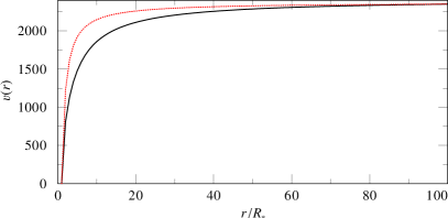
The adopted velocity field in the model consists of two parts. In the inner part, the hydrostatic equation is integrated with the stratification of temperature and mean particle mass, yielding the density stratification. The velocity in this part of the wind is then defined via the continuity equation. This hydrostatic part of the atmosphere is connected smoothly to the wind, with the so called double-$\beta$-law (Hillier & Miller, 1999). The double-$\beta$-law consists of the sum of two beta-law terms with different exponents $\beta_{1}$ and $\beta_{2}$, each of them contributing a pre-specified fraction to the total wind velocity. Compared to the standard “one-beta” law, this allows for a smaller velocity gradient in the lower part of the wind, while the second term, for which we adopt always $\beta_{2}=6$ and a contribution of 35% to the final velocity, causes some noticeable acceleration even at relatively large distances from the star (Fig. 1). The values for $\varv_{\infty}$ and $\beta_{1}$, as included in Table 1, were also adopted from the references.

In the PoWR models the lines are broadened by thermal and microturbulent motion with $\varv_{\rm D}=20\,\mathrm{km}/\mathrm{s}$. In addition, radiation damping and pressure broadening are accounted for in the formal integral.

3.3 Clumping in the 1-D wind model

In our PoWR models, the wind inhomogeneities are treated in the microclumping approximation (for more details see Hamann & Koesterke, 1998). The matter density in the clumps is enhanced by a factor $D=1/f_{V}$, where $f_{V}$ is the fraction of volume filled by clumps. In the present study, we allow the clumping factor to depend on radius, starting to deviate from the homogeneous wind ($D=1$) at about the sonic point ($5\leavevmode\nobreak\ \mathrm{km}/\mathrm{s}$) and quickly reaching $D=10$ at $\varv(r)=40\leavevmode\nobreak\ \mathrm{km}/\mathrm{s}$.

4 3-D clumped wind model

Figure 2: Snapshot from a 3-D Monte-Carlo simulation, showing in two-dimensional projection an example of a clumps realization (red full circles) in respect to star (yellow dashed circle) and the path of a line-scattered photon (blue dotted line).

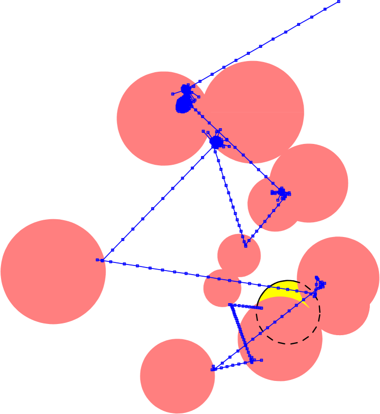
To model the P v resonance line profiles, we use our Monte-Carlo code for the radiative transfer in a three-dimensional clumped wind. In the spirit of a core-halo approximation, the lower boundary of the wind is placed just above the photosphere. Here we employ the photospheric line spectrum as obtained from the PoWR model as inner boundary.

In the wind, we create a random distribution of spherical clumps. These clumps move with the wind velocity law, but have also an additional internal velocity gradient (see below). The number density of clumps obeys the continuity equation. The density in the clumps and in the inter-clump medium is specified from the mass-loss rate and the clumping parameters.

Table 3: Finally adjusted stellar and wind parameters. $\dot{M}_{\text{vink}}/\dot{M}$ is the ratio of theoretical ($\dot{M}_{\text{vink}}$, Vink et al. 2000) to measured ($\dot{M}$) mass-loss rates.

​​​ Star	distance	$R_{V}$	$\dot{M}$	$\dot{M}_{\text{vink}}/\dot{M}$
	[$\mathrm{kpc}$]		[$10^{-6}\leavevmode\nobreak\ \mathrm{M}_{\odot}/\mathrm{yr}$]
​​​ HD 66811	2.34	3.10	2.51	1.86
HD 15570	2.34	3.10	2.75	2.58
HD 14947	3.00	2.80	2.82	2.32
HD 210839	0.95	3.15	1.62	1.78
HD 192639	2.00	3.10	1.26	1.34

The photons which are now released at the lower boundary travel through the wind, where they can be repeatedly scattered in the considered line doublet (continuum opacities are neglected). The line scattering is assumed to be isotropic in the co-moving frame of reference, while the frequencies are completely redistributed over the Doppler-broadened opacity profile. The opacity is computed according to the mass-loss rate, element abundance, and ionization fraction. The latter is retrieved from the PoWR model. Traveling photons experience Doppler shifts due to the wind expansion. Once a photon crosses the outer boundary of the wind it is counted for the emergent profile. The principle of this formalism is illustrated in Fig. 2, while more details of the code are given in Šurlan et al. (2012b).

Table 4: Fixed model parameters used in the 3-D Monte-Carlo code.

​​​ Model parameters	Value
​​​ Inner boundary of the wind	$r_{\text{min}}$	=	$1\,R_{*}$
Outer boundary of the wind	$r_{\text{max}}$	=	$100\,R_{*}$
Clump separation parameter	$L_{0}$	=	0.5
Clumping factor	$D$	=	$10$
Onset of clumping	$r_{\text{cl}}$	=	$1\,R_{*}$
Velocity at the photosphere	$\varv_{\text{min}}$	=	10 [$\mathrm{km}/\mathrm{s}$]
Doppler velocity	$\varv_{\text{D}}$	=	20 [$\mathrm{km}/\mathrm{s}$]

Figure 3: The upper and the middle panels show the synthetic spectra (dotted-black lines) of HD 66811 (left panels) and HD 15570 (right panels) obtained from the PoWR models, i.e. without macroclumping. Thin solid-blue lines are observed spectra. The dashed-green lines in the middle panels are from the same model, but only accounting for the photospheric lines while wind lines from P v and Si iv are suppressed. These photospheric spectra are used as input for the 3-D Monte-Carlo calculations with macroclumping (lower panels). The parameters of these models are given in Tables 1-5.

A set of parameters describes the inhomogeneous wind. The clumping factor $D$ specifies the density inside clumps in respect to the smooth wind density. We used the same value as in the PoWR code for the microclumping. Other clumping properties are the clump separation parameter $L_{0}$, the density of the inter-clump medium $d$ (for the case of a two component medium), and the radius $r_{\text{cl}}$ where clumping sets on. The velocity range inside each clump is described by the velocity deviation parameter $m=\varv_{\text{dis}}(r)/\varv(r)$. For a more detailed description of these parameters we refer to Šurlan et al. (2012b).

5 Model fitting

For each star from the sample, we perform the following procedure:

1. 1-D models are calculated with the PoWR code in order to establish the mass-loss rate from fitting the H$\alpha$ line;

2. then, the obtained mass-loss rate together with the P v ionization fraction and the photospheric spectrum are used as input for the 3-D Monte Carlo simulations of the clumped wind. From optimizing the fit of the P v resonance doublet, the clumping parameters are determined.

These steps are described in more detail in the next two subsections.

Figure 4: Same as Fig. 3 but for HD 14947 (left panels) and HD 210839 (right panels).

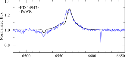
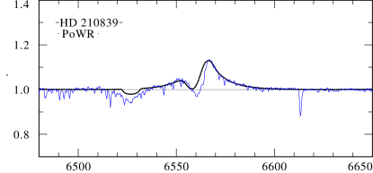
5.1 1-D PoWR model fitting

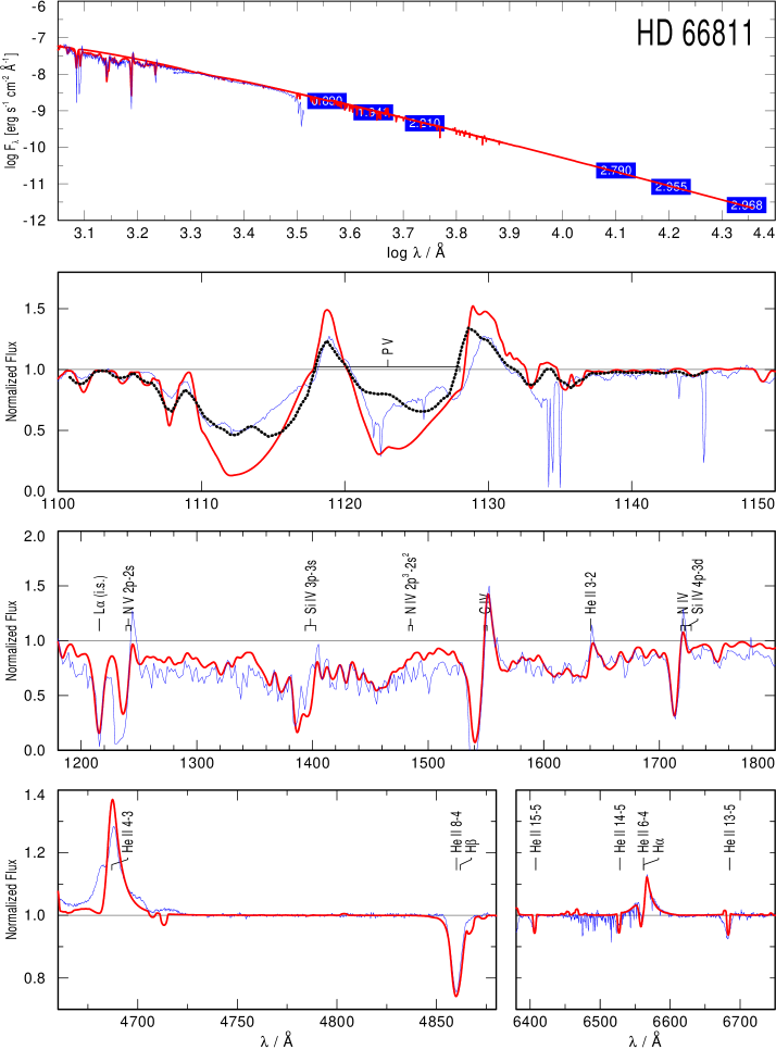
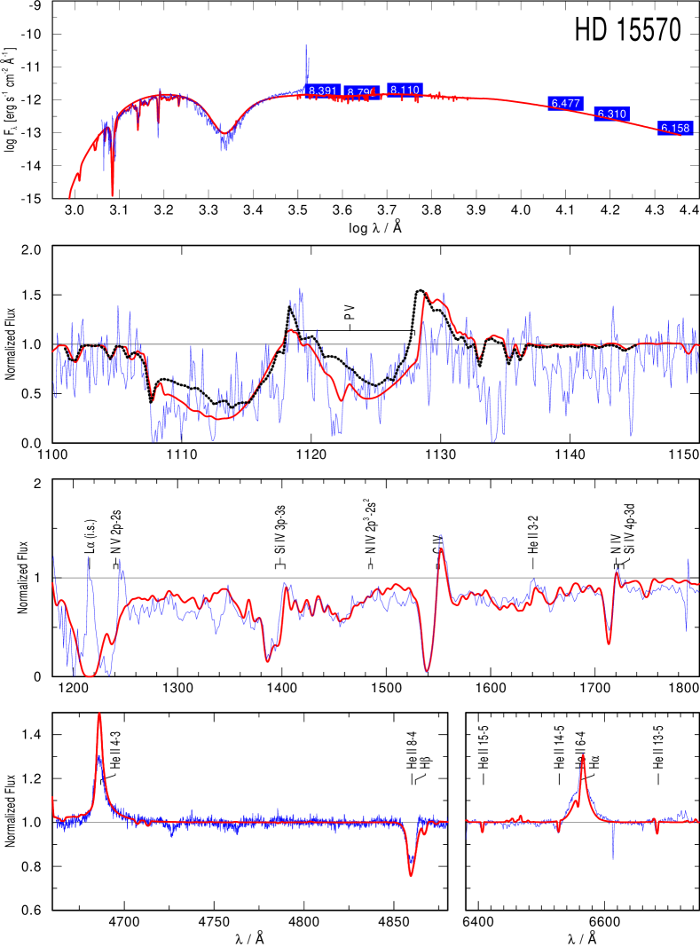
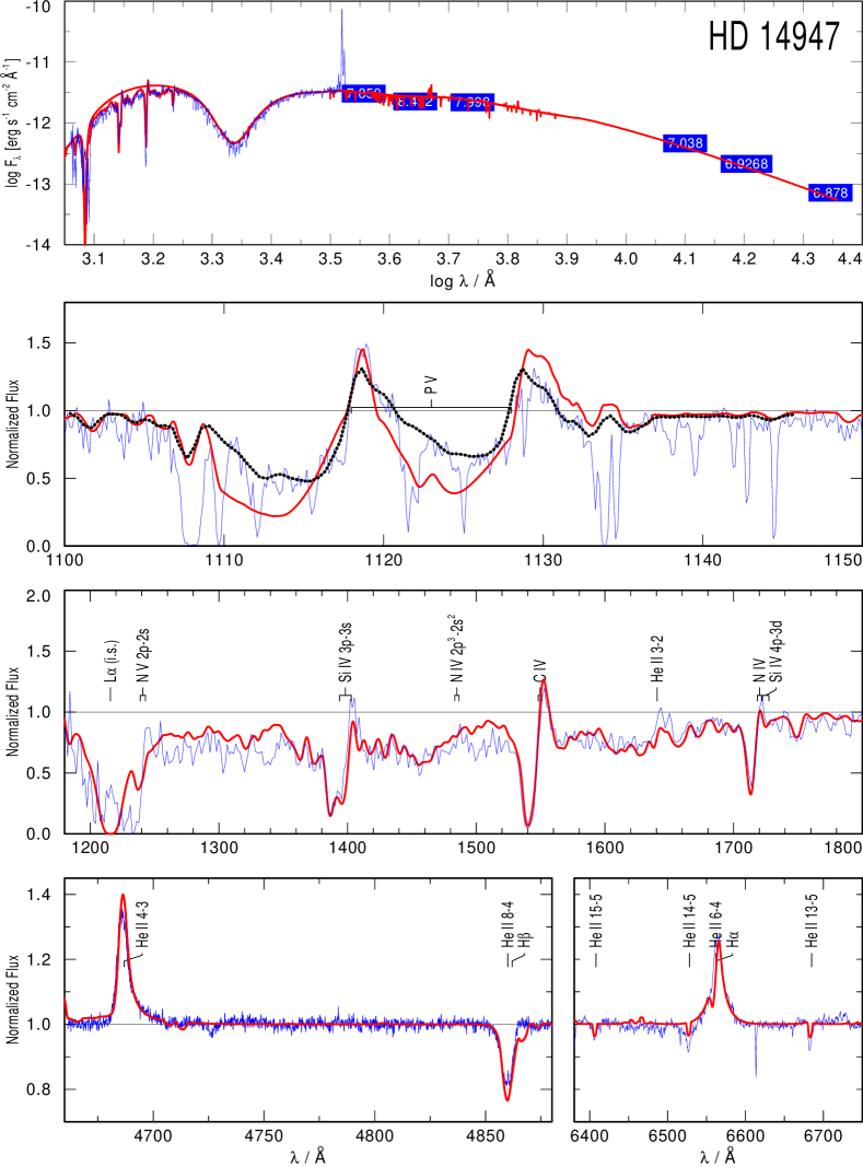
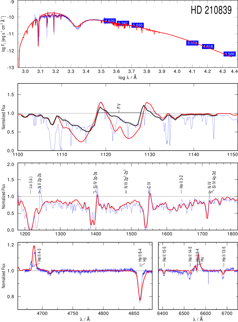
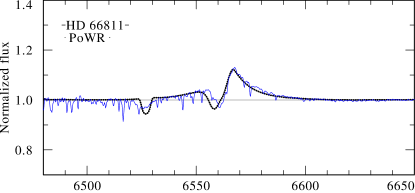
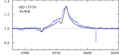
As input to the 1-D PoWR model calculations we used the stellar and wind parameters and element abundances as compiled in Table 1. The mass-loss rates were slightly adjusted in order to optimize the fit with the optical observations (H$\alpha$, H$\beta$, H$\gamma$, and He ii lines). The finally adopted $\dot{M}$ are listed in Table 3.

All spectral fits are documented in the Online Material. Note that the synthetic spectra were flux-convolved to simulate instrumental and rotational broadening, taking $\varv\sin i$ from Bouret et al. (2012).

The UBVJHK photometry of all stars is taken from the GOS catalog (Maíz-Apellániz et al., 2004). The color excess $E_{\rm B-V}$ is adopted from Bouret et al. (2012). We applied the reddening law from Cardelli et al. (1989) and adjusted the $R_{V}$ parameter to optimize the fit between the Spectral Energy Distributions (SED) of the model and the flux-calibrated observations. Moreover, since we kept the luminosity at the literature value, we adjusted the stellar distances to achieve the SED fits. Our final values for $R_{V}$ and the stellar distance are listed in Table 3. The SED fits are documented in the upper panels of Figs. A.1-5 in the Online Material.

5.2 3-D Monte-Carlo model fitting

Table 5: Clumping parameters which give the best fit to the observed P v line profiles. All other model parameters are given in Table 4.

​​​ Star	$d$	$m$
​​​ HD 66811	0.15	0.25
HD 15570	0.40	0.20
HD 14947	0.20	0.10
HD 210839	0.15	0.01
HD 192639	0.10	0.01

Figure 5: Same as Fig. 3 but for HD 192639.

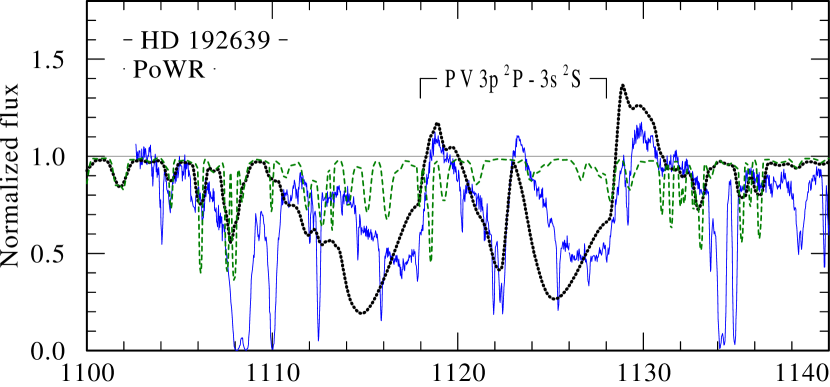
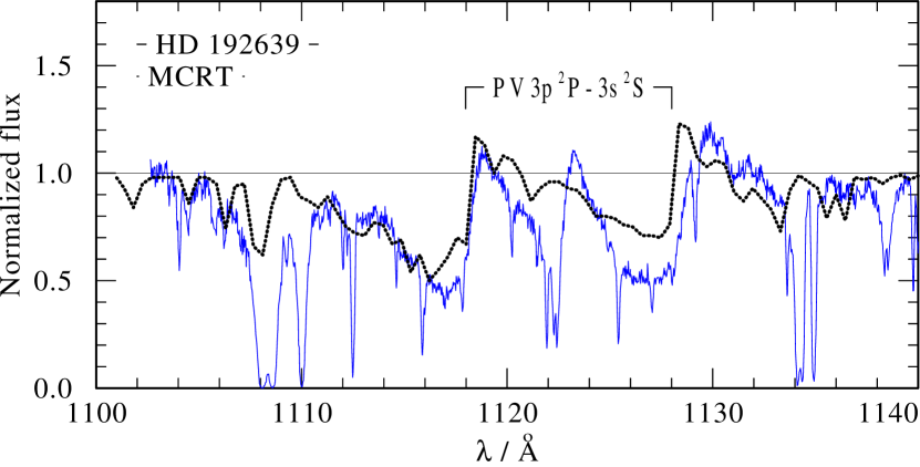
Once the mass-loss rate is established from the $H\alpha$ fitting, the stratification of the P v ionization fraction and photospheric spectra is extracted from the final PoWR model, and used as input for calculating the 3-D Monte-Carlo radiative transfer in the clumped wind as described in Section 4.

To be consistent to the PoWR models, the velocity of the wind is described by a double-$\beta$-law with the same parameters. The clumping factor $D$ and the Doppler-broadening velocity is taken consistent to the PoWR models.

While some of the clumping parameters are fixed (see Table 4), the inter-clump medium density factor $d$ and the velocity deviation parameter $m$ are varied in order to find the best fit to the observed P v doublet. Their final values are given in Table 5.

6 Results

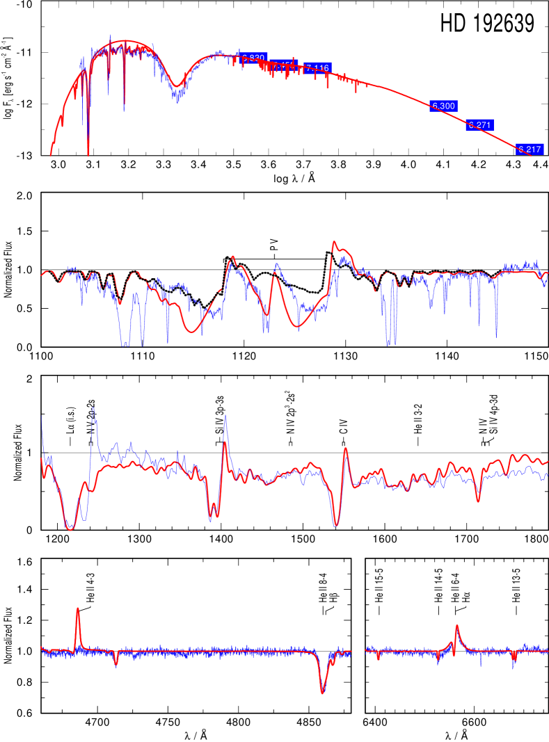
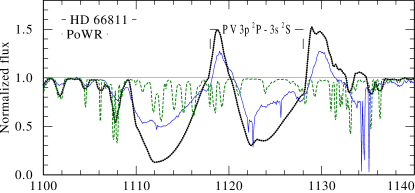
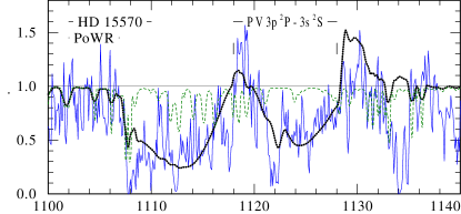
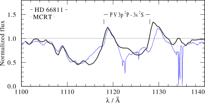
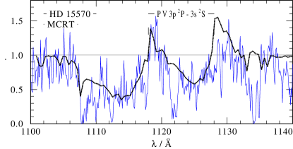
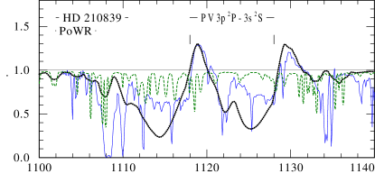
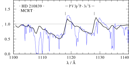
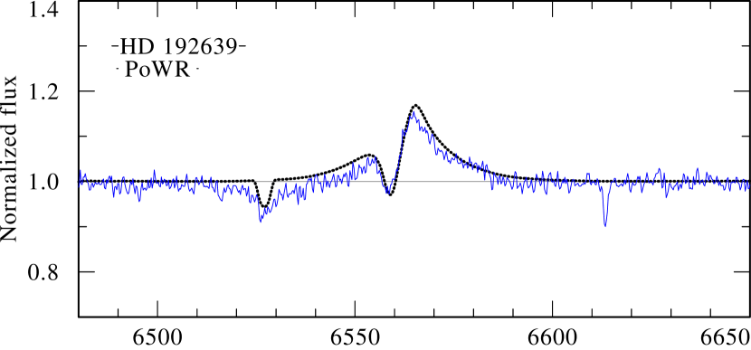
Let us first review the global results of the modeling. As it can be seen from the upper panels of Figs. 3-5, the H$\alpha$ line fits reasonably well, although not perfectly (see also H$\beta$ and He ii profiles in Online material). Comparing our fits with the fits obtained in other investigations, e.g. by Bouret et al. (2012) for the star HD 210839, our fits are not worse. Both our PoWR models and the models of Bouret et al. assumed microclumping throughout the wind. The overall shape of the H$\alpha$, H$\beta$, and He ii 4686 Å lines is fitted well.

For an additional check of the fit, we compare the synthetic UV spectrum with low-resolution IUE spectra (third panels in Figs.10 – 14). All lines fit well except of the N v resonance doublet. This line is partly formed in the tenuous inter-clump medium (Zsargó et al., 2008) which is not included in the PoWR model calculations.

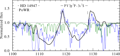
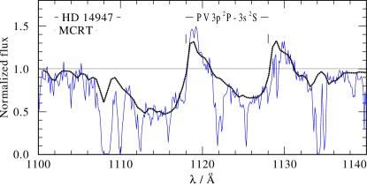
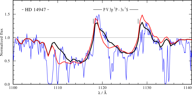
The P v resonance doublet, however, is predicted far too strong by the PoWR models in all cases (see Figs. 3-5, middle panels). In contrast, excellent agreement with observation is achieved with the 3-D Monte-Carlo simulations (see Figs. 3-5, lower panels). The disagreement in the red component of the P v $\lambda\lambda\leavevmode\nobreak\ 1118,1128\leavevmode\nobreak\$Å line for the star HD 192639 (Fig. 5) is caused by blending with the Si iv 1128 Å line, which is not included in our 3-D Monte-Carlo simulations.

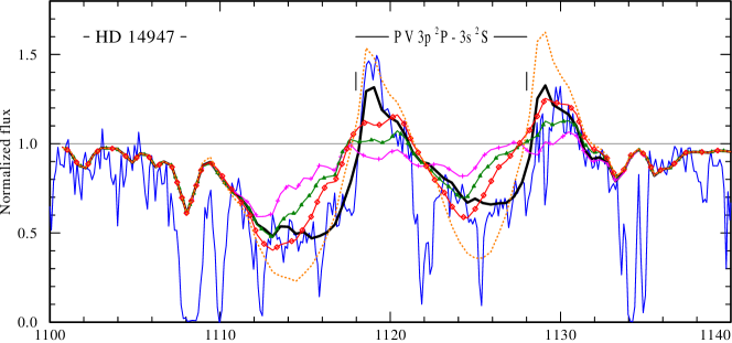
In the following subsections we describe how we chose the clumping parameters for achieving the best agreement between calculated and observed P v profiles. We demonstrate the effect of these parameters by taking HD 14947 as example.

Figure 6: Comparison between calculated P v and observed (thin solid-blue lines) line profiles of HD 14947. Upper panel: Effect of the number of clumps. The purple line with crosses is calculated with $d=0$, $r_{\text{cl}}=1$, $m=0.1$, and $L_{0}=0.5$. The green line with triangles and the red line with squares differ only by $L_{0}=0.2$ and $L_{0}=0.1$, respectively. The thick solid-black line is calculated with $r_{\text{cl}}=1$, $m=0.1$, $L_{0}=0.5$, and $d=0.2$. The dotted orange line is from the PoWR model and corresponds to a smooth wind. Lower panel: Effect of the onset of clumping and the inter-clump medium density. The green line with triangles is calculated with $d=0$, $r_{\text{cl}}=1.1$, $m=0.1$, and $L_{0}=0.5$. The red line with asterisks differs only by $d=0.1$, while the thick solid-black line is for $d=0.2$ and hence differs against the thick solid-black line in the upper panel only by the different $r_{cl}=1.1$. The remaining clump parameters are fixed as given in Table 4.

Figure 7: Dependence of the P v profile on the clumping factor $D$. All four calculations are for $r_{\text{cl}}=1$, $L_{0}=0.5$, $d=0.2$, and $m=0.1$. The thick solid-black line is for our standard value $D=10$. The red line with asterisks shows the profile for $D=5$, the green line with triangles for $D=50$, and the dashed-orange line for $D=400$. The thin solid-blue line is the observed spectrum.

Figure 8: Upper panel: The effects of the “vorosity” on the P v profile. All three calculations are for $L_{0}=0.5$ and $d=0.2$. The green line with triangles shows the profile for $m=0.01$, the red line with asterisk for $m=0.3$, and the thick solid-black line for $m=0.1$. Lower panel: P v line profiles calculated with standard $\beta$-law and constant ionization fraction $q_{{P\textsc{v}}}=1$ (dotted-red line), compared to the simulation with double-$\beta$-law and the ionization stratification from the corresponding PoWR model (thick solid-black line). Both profiles are calculated for $L_{0}=0.5$, $d=0.2$, $r_{\text{cl}}=1$, and $m=0.1$. The thin solid-blue lines in the panels are the observed spectrum. $\lambda_{1\infty}$ and $\lambda_{2\infty}$ represent the wavelength associated with the assumed $\varv_{\infty}$.

6.1 Number of clumps

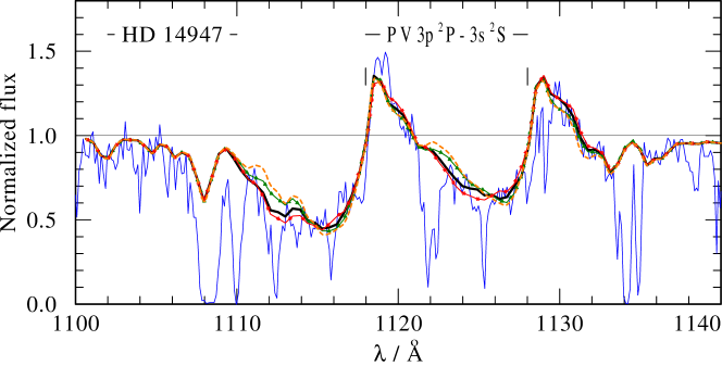
The clump separation parameter $L_{0}$ controls the number of clumps, $N_{\text{cl}}$, in the wind. Decreasing this parameter causes more clumps. For very small $L_{0}$ ($L_{0}\rightarrow 0$), the smooth wind is approached (dotted orange line in the upper panel of Fig. 6). It can be seen that with the smooth wind approximation the absorption is deeper and the emission peaks are higher. For a better fit with observation, we adopt the clumped-wind model and set $L_{0}=0.5$. This implies $1.13\times 10^{4}$ clumps within $100\,R_{*}$ (cf. equation 24 in Šurlan et al. 2012b). The calculated line profile (purple line with crosses in the upper panel of Fig. 6) is drastically reduced.

Now we increase the number of clumps, setting $L_{0}=0.2$ which implies $1.75\times 10^{5}$ clumps within $100\,R_{*}$. Again, neither the strength of the emissions nor the depth of absorptions can be reproduced (green line with triangles in the upper panel of Fig. 6). Even when we create as many as $1.4\times 10^{6}$ clumps in the wind by setting $L_{0}=0.1$ (the red line with squares in the upper panel of Fig. 6), the observed P v line profile is not reproduced.

One may compare these numbers with independent estimates for the number of clumps. E.g., Nazé et al. (2013) recently found that more than $10^{5}$ clumps are required in the wind of HD 66811 in order to explain its very low level of stochastic X-ray variability.

6.2 Inter-clump medium density

For a satisfactory fit of the observed P v profile, additional matter must be located between the clumps. The inter-clump medium density parameter $d$ (see Sect. 2.1.2. in Šurlan et al., 2012b) defines its density. We find that a reasonable fit to the observation can be achieved this way, even with a lower number of clumps. We set $L_{0}=0.5$ and then increase $d$ until satisfactory agreement is reached with about $d=0.2$ (solid-black line in the upper panel of Fig. 6).

If we decrease $L_{0}$ (i.e. larger number of clumps), this can be compensated by smaller values of $d$ to reproduce observation. Hence different combinations of $L_{0}$ and $d$ may give equally good agreement with observation. From our clumped wind model it is not possible to tell with certainty which combination of $L_{0}$ and $d$ corresponds to reality. We can only say that for winds which consist of less than about $10^{6}$ clumps, inter-clump medium density is a necessary ingredient of the wind in order to satisfactorily reproduce the P v resonance doublet. But in any case, the inter-clump space cannot be void.

6.3 Onset of clumping

The parameter $r_{\text{cl}}$ controls the radius where clumping sets on. Since Sundqvist & Owocki (2013) showed that structures in the wind may develop already very close to the wind base at $r_{\text{cl}}\lesssim 1.1\,R_{*}$, we check which effect the onset of clumping may have on the calculated line profile.

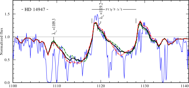
First, we assume a one-component wind ($D=10$, $d=0$) and adopt the $r_{\text{cl}}=1.1\,R_{*}$. As a result, absorption dips appear close to the laboratory wavelength of both P v doublet components (green line with triangles in the lower panel of Fig. 6). To get rid of these sharp absorptions, we set the inter-clump density to $d=0.1$. The result (red line with asterisks in the lower panel of Fig. 6) shows that the absorption dips almost disappear, but still the level of absorption is not fitted well. However, after increasing the inter-clump density to $d=0.2$, the absorption totally disappears, and the level of absorption is reproduced (solid-black line in the lower panel of Fig. 6).

The reason for this effect is that the inter-clump medium above $r_{\text{cl}}$ shields the lower, smooth part of the wind. If the former is dense enough (like for $d=0.2$), both absorption and emission are strong there to hide the layers below.

If we compare the solid-black lines in the upper and lower panels of Fig. 6, which differ only by $r_{\text{cl}}$, we cannot say which line fits the observations better, as both give good agreement with observation. Even if we set $r_{\text{cl}}=1.3\,R_{*}$ and a bit different value of $d$, the agreement with the observed line remains similar. Hence, with appropriate values of $d$, the P v line profile can be fitted equally well regardless if clumping starts from the surface of the star or a bit above. The inter-clump medium hides the spectral signature of the onset of clumping. Non-void inter-clump medium has to be assumed always to fit the overall shape of the P v profile.

For our final models presented in this paper we assume that clumping starts at the base of the wind, for both the PoWR and the Monte-Carlo simulations.

6.4 Dependence on the clumping factor $D$

The parameter $D$ defines the density inside clumps with respect to the smooth wind density. To check how different values of $D$ influence formation of the P v resonance line profile, we varied this parameter for one selected model (HD 14947). The value $D=10$ gives a good fit to the observation (see left panel of Fig. 4). In Fig. 7 we now compare the profiles resulting for different values of $D$ between $5$ to $400$. While a slight preference exists for the fit with our standard value $D=10$, the results depend only little on that parameter. In our previous paper we demonstrated that enhancing the clump density parameter $D$ leads to a more pronounced porosity effect (cf. figure 6 in Šurlan et al., 2012b). Since in this work we include the inter-clump medium, this dependence is apparently reduced.

6.5 Velocity dispersion inside clumps

The porosity effect in the line radiation transfer depends on the gaps in frequency between the line absorption of the individual clumps. This kind of porosity in the velocity coordinate is sometimes called “vorosity” (Owocki, 2008). To investigate this effect, we study the impact of the velocity deviation parameter $m$ (see equation. 20 and figure 3 in Šurlan et al. 2012b), which allows the velocity inside the clumps to deviate from the monotonic dependence on radius. As indicated by hydrodynamic simulations, the velocity gradient is assumed to be negative there, while the ambient inter-clump medium is moving monotonically according to the wind velocity law.

The effects of $m$ on the P v line profile are shown in Fig. 8. From our modeling follows that “vorosity” mainly affects the outer part of the wind, extending the absorption beyond $\varv_{\infty}$ and leading to a softening of the blue edge. In all stars of the sample, this improves the fit. However, we do not find any significant reductions of the overall line strength. On the other hand, Sundqvist et al. (2010) found vorosity of similar importance as porosity. We can not confirm their conclusion.

Figure 9: Influence of velocity law and ionization fraction of P v on profiles of the P v resonance doublet. Profiles are calculated with $d=0.2$, $r_{\text{cl}}=1$, $m=0.1$, and $L_{0}=0.5$ for the case of HD 14947. Upper panel: Comparison of profiles of the P v doublet for standard $\beta$-law (the dotted-red line) and double-$\beta$-law (solid-black line). Lower panel: Comparison of profiles of the P v doublet for constant ionization fraction $q_{{P\textsc{v}}}=1$ (the dotted red line) and ionization fraction following from the double-$\beta$-law (the thick solid black line). The thin solid blue line is the observed spectrum.

6.6 Clumping parameter degeneracies

In our models, we are using several free parameters describing the properties of clumping ($L_{0}$, $D$, $d$, $r_{\text{cl}}$, $m$). However, it happens that for some different combinations of clumping parameters we obtain similar or exactly the same P v line profiles. There is a question, if it is possible to break such degeneracies of parameters. This is quite a complicated problem. Using a single line it is probably impossible. However, adding more lines to the analysis with different line opacities and different depths of formation may put some additional constraints on the adopted set of parameters. For example, Zsargó et al. (2008) showed that the O vi $\lambda\lambda\leavevmode\nobreak\ 1032,1038$ resonance doublet (created by Auger ionization by X-rays from O iv) could be used to characterize the inter-clump medium and break the degeneracy in the interpretation of fits to the P v doublet. However, their conclusion is based on 1-D wind model assuming microclumping (consequently with less free parameters) and requires verification for the more general case of a 3-D geometry. It is an interesting problem, which goes beyond the scope of the present paper, but we intend to study it in future by simultaneous fitting of P v and O vi doublets using their ionization structure obtained from PoWR model, provided we find appropriate observational data. Despite the fact that it is difficult to disentangle parameters of our model, our key conclusion is the accordance different mass-loss rate diagnostic when macroclumping is included in the models.

6.7 Velocity law and P v ionization stratification

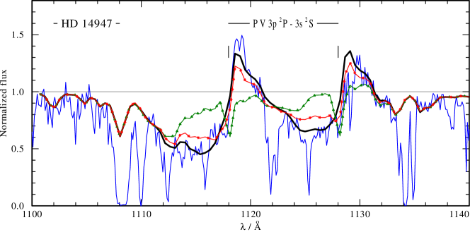
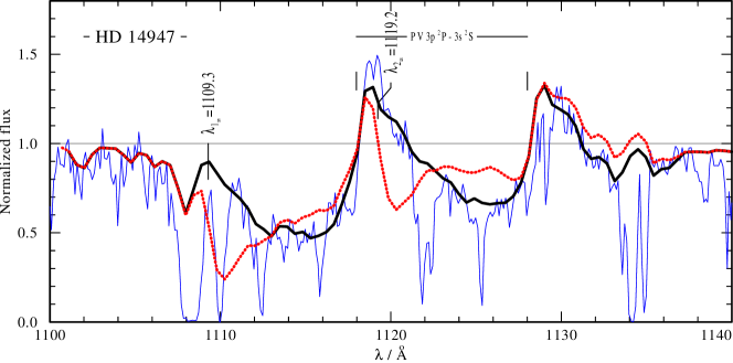
In our models we prefer the so called double-$\beta$-law (cf. Sect. 3.2). The main motivation for adopting the double-$\beta$-law is to get rid of the absorption dip close to the the blue edge of the profile, which appears notoriously in models with the standard $\beta$-law. With the double-$\beta$-law, the persistent acceleration in the outer wind enhances the velocity gradient there, and thus reduces the line optical depth at largest blueshifts. A physical reason for such dynamic behavior was suggested already by Lucy & Abbott (1993), who speculated that such a persistent acceleration could arise from changes in the ionization structure. The mentioned blue edge absorption dip is clearly seen in Fig. 9 (upper panel), where the dotted-red line shows the calculation with the one-$\beta$-law, and the solid-black line with the double-$\beta$-law.

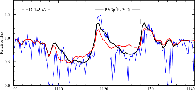
In the lower panel of Fig. 9 we demonstrate the influence of the ionization stratification. The red-dotted profile is calculated with constant $q_{{P\textsc{v}}}=1$ in the whole wind, while for the thick solid-black line the ionization stratification has been taken from the corresponding PoWR model. For the parametric range of the stars in our sample, the PoWR models predict that more than $80\%$ of phosphorus is in ionization stage of P v, except close to the photosphere. The double-$\beta$-law was employed in both cases. As can be seen, the decrease of the P v ionization fraction results in a shallower absorption in the outer wind.

7 Discussion

7.1 Clumping in the inner wind

Time-dependent 1-D hydrodynamic models of radiation-driven winds always predicted that the line de-shadowing instability grows only in the acceleration zone. Thus, strongly inhomogeneous structures were expected to develop only at radii $r_{\text{cl}}\gtrsim 1.3\,R_{*}$ (Feldmeier et al., 1997; Runacres & Owocki, 2002; Dessart & Owocki, 2005). Recently, however, Sundqvist & Owocki (2013) obtained structures already close to the wind base ($r_{\text{cl}}\lesssim 1.1\,R_{*}$), when they accounted for the effect of limb darkening.

There are observational arguments to suggest that clumping may start close to the stellar surface (e.g. Puls et al., 2006). The early onset of clumping close to the stellar photosphere may be a consequence of the subsurface convection as investigated by Cantiello & Braithwaite (2011). The presence of X-ray emission very close to the photosphere (Waldron & Cassinelli, 2007) is an argument to support these considerations.

In our last paper (Šurlan et al., 2012b) we also concluded that clumping sets on close to the wind base, because otherwise deep, un-shifted absorption features should be seen in the P v resonance doublet which are not observed. In the light of our present results, this conclusion is not so firm anymore. As mentioned in Sect. 6.3, the observations can also be reproduced if we assume $r_{\text{cl}}=1.3\,R_{*}$, while setting the inter-clump medium parameter to $d=0.2$. Obviously, the inter-clump medium reprocesses the radiation coming from the base of the wind. Hence it is not possible to tell if the lower wind is already clumped or not, at least not for the relatively dense supergiant winds investigated here.

7.2 Clumping in the outer wind

The hydrodynamic simulations of the line de-shadowing instability mentioned above predict that the clumps persist to large distances from the star. This justifies our assumption that clumping extends to large radii, even to $r_{\text{max}}\gtrsim 100\,R_{*}$.

Smooth-wind models predict much deeper absorption in the blue part of the line profile than observed (see Fig. 8). Obviously, the effective opacity in the outer part of the wind is over-estimated. Most importantly, we showed that this opacity can be effectively reduced by the porosity effect. Additionally, the correct ionization fraction of P v lowers the absorption a bit, and the double-$\beta$-law distributes the line opacity more uniformly across the line profile.

Our 3-D Monte-Carlo radiative transfer calculations were performed with constant clumping parameters throughout the wind, which implies that the clumps become larger and more separated from each other with growing distance from the star. We should note here that the clumping parameter $D$ may in fact be depth dependent (see Puls et al., 2006).

7.3 P v ionization fraction

The importance of the P v ionization fraction was pointed out by Crowther et al. (2002). The studies which had stated the mass-loss rate discrepancy (Massa et al., 2003; Fullerton et al., 2006) have used simplified methods for simulating the P-Cygni profiles of the P v resonance doublet, namely the “Sobolev with exact integration” (SEI) method (Lamers et al., 1987). For this approach, the ionization fraction of the P v ion must be adopted, and has been assumed to be constant throughout the wind and close to unity (i.e., all phosphorus is in the P v ground state). Our detailed non-LTE models show that the ionization fraction of P v is actually somewhat lower, and can vary with radius.

Additionally, the ionization fraction of P v may be affected by X-rays. This influence was examined by Krtička & Kubát (2009) who showed that X-rays of the observed intensity cannot deplete the P v ionization fraction significantly. Still, Waldron & Cassinelli (2010) suggested that strong emission line radiation in the XUV energy band can significantly reduce the abundance of P v and thus explain the discrepant low mass-loss rates estimates. However, Krtička & Kubát (2012) showed that if the XUV radiation would be strong enough to reduce the ionization fraction of P v, it would also change the ionization balance of other elements and significantly reduce the wind driving force, consequently also stellar mass-loss rates.

Here we performed tests by including an X-ray field into the PoWR calculations, using the parameters of X-ray radiation as obtained from observations (Oskinova et al., 2006). . We confirm the result found by Krtička & Kubát (2009) that the X-rays really have no effect on the ionization balance of phosphorus, especially on the abundance of P v. Similar conclusions were also drawn by Bouret et al. (2012).

7.4 Mass-loss rates

In principle, mass-loss rates through radiatively driven stellar winds can be predicted from adequate hydrodynamical models. Ideally, such models would yield $\dot{M}$ and $\varv_{\infty}$ from a given set of stellar parameters (stellar luminosity, mass, radius, and chemical composition). Practically, such codes have to accept severe approximations. In most of them, the radiative force is parameterized using the so-called force multipliers (see Castor et al., 1975; Abbott, 1982). Some of these codes calculate the radiative force in detail from a list of spectral lines (Krtička & Kubát, 2004, 2009, 2010).

Hydrodynamical stellar wind models which account for clumping are still missing. In a few test calculations, Krtička et al. (2008) and Muijres et al. (2011) studied the effect of clumping on the radiative force.

Vink et al. (2000) performed Monte-Carlo calculations of the radiative force, also using detailed line lists. However, they assumed the velocity law, instead of a fully consistent hydrodynamical solution. Conveniently, they condensed their results into a fit formula, which is widely used as reference for mass-loss rates.

Therefore we also compare our mass-loss rates, which are consistent with the H$\alpha$ emission and the un-saturated UV resonance doublet of P v, with the Vink formula (Table 3, last column). On the average, our mass-loss rates are smaller by a factor of two.

However, one should keep in mind that our $\dot{M}$ relies on the assumption that the clumping contrast is $D=10$. Within some range of $D$ a simultaneous fit of H$\alpha$ and P v may be possible as well, with somewhat different mass-loss rates $\dot{M}\propto D^{-1/2}$.

8 Summary

For a sample of five O-type supergiants, we studied the effects of wind clumping on the mass-loss rate determination, considering simultaneously the H$\alpha$ emission (and other Balmer and He ii lines) and the un-saturated resonance doublet of P v in the far-ultraviolet.

• When accounting for macroclumping, it is possible to simultaneously fit the H$\alpha$ and the P v lines with the same mass-loss rates.

• The consistent fit is achieved when we simulate the P v resonance profile with our 3-D Monte-Carlo code for the line radiation transfer in clumpy stellar winds. Obviously, the reported discrepancies between H$\alpha$ and P v mass-loss rates were due to the inadequate treatment of clumping.

• The mass-loss rates for our consistent fits are lower by a factor of 1.3 to 2.6, compared to the mass-loss formula by Vink et al. (2000).

• In contrast to other studies, it was neither necessary to reduce the mass-loss rate by adopting an extremely high degree of clumping, nor to assume a sub-solar phosphorus abundance for our consistent fits.

• The porosity that is needed to fit the P v lines implies that $\sim 10^{4}$ clumps populate the wind within $100\,R_{\ast}$ at a given moment.

• The velocity dispersion inside the clumps has a moderate effect on the porosity of the wind, and hence on the P v profile. The smaller this dispersion, the smaller is the effective line opacity.

• Compared to the standard $\beta$-velocity law, the double-$\beta$ law improves the detailed fit of the P v line profile. It smooths the blue absorption edge and removes the absorption dip close to that edge.

• With the detailed ionization stratification of P v from the PoWR code, a better agreement with observed P v line profile can be achieved than with $q_{{P\textsc{v}}}\equiv 1$.

Our results emphasize that an adequate treatment of the line formation in inhomogeneous winds is prerequisite for the interpretation of O-star spectra and the determination of mass-loss rates.

Appendix A Spectral fits

Figure 10: Best fit from PoWR modeling (thick red-solid lines) to the observed HD 66811 spectra (thin blue-solid lines) together with the calculated P v line profile from 3-D Monte-Carlo code (black-dotted line). Blue labels with numbers in the upper panels are UBVJHK magnitudes.

Figure 11: The same as Fig. 10, but for HD 15570.

Figure 12: The same as Fig. 10, but for HD 14947.

Figure 13: The same as Fig. 10, but for HD 210839.

Figure 14: The same as Fig. 10, but for HD 192639.

References

- Abbott (1982) Abbott, D. C. 1982, ApJ, 263, 723
- Asplund (2005) Asplund, M. 2005, ARA&A, 43, 481
- Asplund et al. (2009) Asplund, M., Grevesse, N., Sauval, A. J., & Scott, P. 2009, ARA&A, 47, 481
- Bouret et al. (2012) Bouret, J.-C., Hillier, D. J., Lanz, T., & Fullerton, A. W. 2012, A&A, 544, A67
- Bouret et al. (2005) Bouret, J.-C., Lanz, T., & Hillier, D. J. 2005, A&A, 438, 301
- Bouret et al. (2003) Bouret, J.-C., Lanz, T., Hillier, D. J., et al. 2003, ApJ, 595, 1182
- Cantiello & Braithwaite (2011) Cantiello, M. & Braithwaite, J. 2011, A&A, 534, A140
- Cardelli et al. (1989) Cardelli, J. A., Clayton, G. C., & Mathis, J. S. 1989, ApJ, 345, 245
- Castor et al. (1975) Castor, J. I., Abbott, D. C., & Klein, R. I. 1975, ApJ, 195, 157
- Crowther et al. (2002) Crowther, P. A., Hillier, D. J., Evans, C. J., et al. 2002, ApJ, 579, 774
- De Becker et al. (2009) De Becker, M., Rauw, G., & Linder, N. 2009, ApJ, 704, 964
- Dessart & Owocki (2005) Dessart, L. & Owocki, S. P. 2005, A&A, 432, 281
- Eversberg et al. (1998) Eversberg, T., Lépine, S., & Moffat, A. F. J. 1998, ApJ, 494, 799
- Feldmeier et al. (1997) Feldmeier, A., Puls, J., & Pauldrach, A. W. A. 1997, A&A, 322, 878
- Fullerton et al. (2006) Fullerton, A. W., Massa, D. L., & Prinja, R. K. 2006, ApJ, 637, 1025
- Hamann & Gräfener (2004) Hamann, W.-R. & Gräfener, G. 2004, A&A, 427, 697
- Hamann & Koesterke (1998) Hamann, W.-R. & Koesterke, L. 1998, A&A, 335, 1003
- Hillier & Miller (1998) Hillier, D. J. & Miller, D. L. 1998, ApJ, 496, 407
- Hillier & Miller (1999) Hillier, D. J. & Miller, D. L. 1999, ApJ, 519, 354
- Krtička & Kubát (2004) Krtička, J. & Kubát, J. 2004, A&A, 417, 1003
- Krtička & Kubát (2009) Krtička, J. & Kubát, J. 2009, MNRAS, 394, 2065
- Krtička & Kubát (2010) Krtička, J. & Kubát, J. 2010, A&A, 519, A50
- Krtička & Kubát (2012) Krtička, J. & Kubát, J. 2012, MNRAS, 427, 84
- Krtička et al. (2008) Krtička, J., Muijres, L., Puls, J., Kubát, J., & de Koter, A. 2008, in IAU Symposium, Vol. 252, The Art of Modeling Stars in the 21st Century, ed. L. Deng & K. L. Chan, 283 – 287
- Lamers et al. (1987) Lamers, H. J. G. L. M., Cerruti-Sola, M., & Perinotto, M. 1987, ApJ, 314, 726
- Lépine & Moffat (2008) Lépine, S. & Moffat, A. F. J. 2008, AJ, 136, 548
- Lucy & Abbott (1993) Lucy, L. B. & Abbott, D. C. 1993, ApJ, 405, 738
- Lucy & Solomon (1970) Lucy, L. B. & Solomon, P. M. 1970, ApJ, 159, 879
- Maíz-Apellániz et al. (2004) Maíz-Apellániz, J., Walborn, N. R., Galué, H. Á., & Wei, L. H. 2004, ApJS, 151, 103
- Markova et al. (2004) Markova, N., Puls, J., Repolust, T., & Markov, H. 2004, A&A, 413, 693
- Mason et al. (1998) Mason, B. D., Gies, D. R., Hartkopf, W. I., et al. 1998, AJ, 115, 821
- Massa et al. (2003) Massa, D., Fullerton, A. W., Sonneborn, G., & Hutchings, J. B. 2003, ApJ, 586, 996
- Meynet & Maeder (2007) Meynet, G. & Maeder, A. 2007, A&A, 464, L11
- Muijres et al. (2011) Muijres, L. E., de Koter, A., Vink, J. S., et al. 2011, A&A, 526, A32
- Nazé et al. (2013) Nazé, Y., Oskinova, L. M., & Gosset, E. 2013, ApJ, 763, 143
- Oskinova et al. (2006) Oskinova, L. M., Feldmeier, A., & Hamann, W.-R. 2006, MNRAS, 372, 313
- Oskinova et al. (2007) Oskinova, L. M., Hamann, W.-R., & Feldmeier, A. 2007, A&A, 476, 1331
- Owocki (2008) Owocki, S. P. 2008, in Clumping in Hot-Star Winds, ed. W.-R. Hamann, A. Feldmeier, & L. M. Oskinova, 121
- Prinja & Massa (2010) Prinja, R. K. & Massa, D. L. 2010, A&A, 521, L55
- Puls et al. (2006) Puls, J., Markova, N., Scuderi, S., et al. 2006, A&A, 454, 625
- Puls et al. (2005) Puls, J., Urbaneja, M. A., Venero, R., et al. 2005, A&A, 435, 669
- Puls et al. (2008) Puls, J., Vink, J. S., & Najarro, F. 2008, A&A Rev., 16, 209
- Pych (2004) Pych, W. 2004, PASP, 116, 148
- Repolust et al. (2005) Repolust, T., Puls, J., Hanson, M. M., Kudritzki, R.-P., & Mokiem, M. R. 2005, A&A, 440, 261
- Runacres & Owocki (2002) Runacres, M. C. & Owocki, S. P. 2002, A&A, 381, 1015
- Sota et al. (2011) Sota, A., Maíz Apellániz, J., Walborn, N. R., et al. 2011, ApJS, 193, 24
- Sundqvist & Owocki (2013) Sundqvist, J. O. & Owocki, S. P. 2013, MNRAS, 428, 1837
- Sundqvist et al. (2010) Sundqvist, J. O., Puls, J., & Feldmeier, A. 2010, A&A, 510, A11
- Sundqvist et al. (2011) Sundqvist, J. O., Puls, J., Feldmeier, A., & Owocki, S. P. 2011, A&A, 528, A64
- Turner et al. (2008) Turner, N. H., ten Brummelaar, T. A., Roberts, L. C., et al. 2008, AJ, 136, 554
- Šurlan et al. (2012a) Šurlan, B., Hamann, W.-R., Kubát, J., Oskinova, L., & Feldmeier, A. 2012a, in Astronomical Society of the Pacific Conference Series, Vol. 465, Astronomical Society of the Pacific Conference Series, ed. L. Drissen, C. Rubert, N. St-Louis, & A. F. J. Moffat, 134
- Šurlan et al. (2012b) Šurlan, B., Hamann, W.-R., Kubát, J., Oskinova, L. M., & Feldmeier, A. 2012b, A&A, 541, A37
- Vink et al. (2000) Vink, J. S., de Koter, A., & Lamers, H. J. G. L. M. 2000, A&A, 362, 295
- Walborn et al. (2009) Walborn, N. R., Nichols, J. S., & Waldron, W. L. 2009, ApJ, 703, 633
- Waldron & Cassinelli (2007) Waldron, W. L. & Cassinelli, J. P. 2007, ApJ, 668, 456
- Waldron & Cassinelli (2010) Waldron, W. L. & Cassinelli, J. P. 2010, ApJ, 711, L30
- Zsargó et al. (2008) Zsargó, J., Hillier, D. J., Bouret, J.-C., et al. 2008, ApJ, 685, L149