A maximum entropy model for opinions in social groups

Abstract

We study how the opinions of a group of individuals determine their spatial distribution and connectivity, through an agent-based model. The interaction between agents is described by a Hamiltonian in which agents are allowed to move freely without an underlying lattice (the average network topology connecting them is determined from the parameters). This kind of model was derived using maximum entropy statistical inference under fixed expectation values of certain probabilities that (we propose) are relevant to social organization. Control parameters emerge as Lagrange multipliers of the maximum entropy problem, and they can be associated with the level of consequence between the personal beliefs and external opinions, and the tendency to socialize with peers of similar or opposing views. These parameters define a phase diagram for the social system, which we studied using Monte Carlo Metropolis simulations. Our model presents both first and second-order phase transitions, depending on the ratio between the internal consequence and the interaction with others. We have found a critical value for the level of internal consequence, below which the personal beliefs of the agents seem to be irrelevant.

I Introduction

Agent-based models have been extensively used to comprehend some aspects of social behavior. In these models, an individual is typically represented either as a (free) particle or as a node in a network with a given topology, to which there is some additional information attached (its inner degrees of freedom). It is interesting to note that there is some overlap with physical models, and this promises to bring new insight to questions such as the possible processes of formation of social groups, what determines their stability and their evolution, in terms of “microscopical details” such as the kinds of interaction among individualsBall (2002); Castellano et al. (2009). Two models in particular have gathered considerable interest and have stood the test of time, these are the Sznajd model for the dynamics of opinions and consensus in a population Sznajd-Weron and Sznajd (2000); Sabatelli and Richmond (2004); Wang et al. (2008), and Axelrod’s model for the dissemination of culture Axelrod (1997); Castellano et al. (2000). Unfortunately, obtaining analytical results from these (and other, similar) models is sometimes a daunting task, so one has to resort to numerical simulations.

Several approaches have been devised for the numerical treatment of agent-based models. Among them we find non-deterministic cellular automata Kacperski and Holyst (1999), variants of the Potts model Liu et al. (2001); Schulze (2005), use of the Langevin equation for the description of stochastic dynamics Hu and Wang (2009), as well as Hamiltonian models Fronczak et al. (2006) together with other tools coming from Statistical Mechanics. Another, completely different line is the use of empirical models in analogy with physical phenomena Ausloos and Petroni (2007, 2009).

Agent-based models present several interesting properties, such as the emergence of different kinds of phase transitions Castellano et al. (2000); Klemm et al. (2003a, b); Fronczak et al. (2007). In these phases we can recognize different regimes (ordered and disordered equilibrium states, metastable states) which appeal to our intuitions about social phenomena. Interestingly, recent studies Biely et al. (2008); Kozma and Barrat (2008); Benczik et al. (2009) have drifted away from fixed-lattice models towards adaptive networks, taking into account the social mobility of individuals.

The central motivation for the present paper has been the development of an agent-based social model of opinion that explicitly incorporates the mobility of individuals in a coherent and least-biased manner. In order to achieve this goal, we have recognized the existence of two important factors which are relevant to the social dynamics: the level of consequence of individuals with respect to their private, internal opinions on a given issue, and the strength and type of coupling between individuals. This coupling can be assortative (meaning the individual tends to be close only to those with the same opinion) or disassortative (where the tendency is the opposite, i.e., to be surrounded only by those with different opinions to their own).

Focusing on just these two aspects of the social phenomena (internal consequence and interaction with others) we have followed the formalism of maximum entropy statistical inference Jaynes (1957) to construct an unbiased probability distribution for the state of our system under known degrees of consequence and coupling. From this probability distribution we deduced the corresponding objective function or Hamiltonian, which the system minimizes in the absence of noise. In the definition of our model, we aim to assume nothing besides the observed qualities of interaction and consequence in agents. The Hamiltonian function by itself provides a complete description of the equilibrium states, including the spatial distribution of agents, the level of homogeneity or diversity of opinions within a society, among other properties. The resulting Hamiltonian resembles the well-known Potts model Wu (1982), and is actually a generalization of it, in which the topology of the lattice is no longer fixed, and where an additional term in the form of a local field is considered. This term introduces a tendency of an individual to resist the influence of its neighbors. The fact that our model lifts the restriction of a fixed lattice (on which agents traditionally “live”) grants the agents a complete freedom of movement and minimizes the number of assumptions.

This paper is organized as follows. In section II we motivate our constraints and derive our model using the maximum entropy formalism. Section III comments on the Hamiltonian thus derived and its resemblance to the Potts Hamiltonian. In section IV we present analytical results as well as Monte Carlo simulations of the phase diagram for our model. Finally we provide some concluding remarks.

II Derivation of the model using statistical inference

Suppose the following. For a given issue there are $Q$ alternative positions or possible opinions an individual can adopt as his/her own. For instance, these could be political views to adhere to, sports teams to support, musical styles people enjoy, and so on. A particular individual could have a preferred choice, which is private to him/her, and could express the same choice, or a different one, to others, for instance depending on social pressure (to “fit in”). For example, consider a political election with just three parties: left-wing, right-wing and independents. An individual with, say, independent views could instead express right-wing views in order to be socially accepted in an exclusive club reunion among mostly right-wing peers. It is natural to think also that some individuals will prefer the company of like-minded peers, sharing the same preferred opinions, while others will seek the company of people with postures different from their own.

In order to construct our mathematical model we will consider $N$ agents (labelled by an index $i=1,\ldots,N$), each one having the following attributes:

1. a continuous position vector $\mathbf{r}_{i}$ in a two-dimensional space,

2. a personal or internal opinion (or belief) $B_{i}$, which represents what the agent “really believes”, and is encoded as an integer between 1 and $Q$, and

3. an external opinion $S_{i}$, which represents what the agent actually expresses in front of others (and is also encoded as an integer between 1 and $Q$).

In the example above, the individual with independent views has $B=$3 and $S=2$. In a social context, definitions (a), (b) and (c) encode the information we have about individuals being free to move around, holding a (sometimes strong) belief about a particular issue and expressing an opinion about said issue. The opinions represented may not represent faithfully what the individuals really believe, and in such cases $S_{i}$ $\neq$ $B_{i}$.

We will assume that the set of internal beliefs $B_{i}$ of the agents are fixed (“quenched”), so that the coordinates of a given agent are only its position and external opinion $S_{i}$. In other words, we are studying the behavior of a particular set of individuals, within a time interval short enough so that none of them has the opportunity to change its belief. Of course, to infer the behavior of a generic population, we would need to marginalize (average over) the belief variables $B_{i}$ under a given statistical model $P(B_{1},\ldots,B_{N}|H)$, for instance, a multinomial distribution.

On the other hand, we will not assume any particular topology or interaction between agents at this point, those will be provided by the maximum entropy inference procedure. However, we will assume that there is some “locality” to the influence in terms of opinions, that is, there is some measure of distance among agents such that a particular agent is only concerned with the opinions of peers closer than a given radius $R_{c}$.

Now, in order to arrive at a well defined Hamiltonian, we need to introduce the main assumptions of the model. The first assumption we will make, besides the existence of all the attributes described above (definitions (a), (b) and (c)), is that the phenomenon of consequence is completely described by the probability of an agent being consequent, i.e., the probability that its internal and external opinion actually agree. This probability can be written in Bayesian notation as $P(S_{i}=B_{i}|H)$ (the $H$ in the conditional is the generic Bayesian “placeholder” for the current context or state of information) and we will denote it shortly by $P_{C}$.

Our second assumption is that the joint probability of agreement and closeness, i.e., that two agents simultaneously agree in opinion ($S_{i}=S_{j}$) and are spatially close ($r_{ij}<R_{c}$), written by $P(S_{i}=S_{j}\wedge r_{ij}<R_{c}|H)$ and denoted by $P_{J}$, is relevant to the phenomenon of assortativity. However, this by itself is not sufficient: for instance, observing a situation where both agreement and closeness is common (Fig. 1, left panel) does not imply the existence of correlation between closeness and agreement. We could also observe situations like the right panel of Fig. 1, and then we infer that in this particular case a tendency to closeness explains everything.

Figure 1: A schematic diagram depicting two states of a system for which we could attempt to infer an assortative association. The left panel is consistent with assortativity, but only until we see the right panel we realize it is only an effect of a tendency for closeness between agents (regardless of their color).

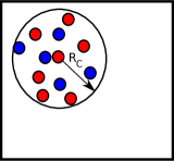
Therefore we will include as a third assumption, the relevance of the probability of closeness, namely $P(r_{ij}<R_{c}|H)=P_{R}$, to a description of the phenomenon of assortative/disassortative association.

We can write all three probabilities as constraints in the form of known expectation values,

$$P(S_{i}=B_{i}|H)=P_{C}=\frac{1}{N}\Big{<}\sum_{i=1}^{N}\delta(S_{i},B_{i})\Big{>}$$ (1)

$$P(S_{i}=S_{j}\wedge r_{ij}<R_{c}|H)=\frac{1}{N(N-1)}\Big{<}\sum_{i=1}\sum_{j\neq i}\Theta(R_{c}-r_{ij})\delta(S_{i},S_{j})\Big{>}$$ (2)

$$P(r_{ij}<R_{c}|H)=\frac{1}{N(N-1)}\Big{<}\sum_{i=1}\sum_{j\neq i}\Theta(R_{c}-r_{ij})\Big{>}$$ (3)

where $\delta(a,b)$ is Kronecker’s delta function and $\Theta(x)$ is Heaviside’s step function. Here we can outline the problem as a case of maximum entropy (MaxEnt) inference Jaynes (1957). The most unbiased estimation of the full probability of being in state $\Gamma$={$S_{1}$,$S_{2}$,…,$S_{N}$,$\mathbf{r}_{1}$,$\mathbf{r}_{2}$,…,$\mathbf{r}_{N}$} is the one that maximizes Shannon’s information entropy

$$\mathcal{S}=-\sum_{S_{1},\ldots,S_{N}}\int d\mathbf{r}_{1}\mathbf{r}_{2}\ldots\mathbf{r}_{N}P(\Gamma|H)\log_{2}\frac{P(\Gamma|H)}{P(\Gamma|H_{0})}.$$ (4)

subjected to the known expectation values at the right-hand side of Eq. 3. Note that, as the $\mathbf{r}_{i}$ are continuous we have to include $P(\Gamma|H_{0})$ as an invariant measure Jaynes (2003) for the configuration space $\Gamma$. We will consider it a constant which does not influence the maximization procedure. The maximum entropy solution for $P(\Gamma|H)$ has the following form,

$$\ln P(\Gamma|H)=-\ln Z+\frac{\lambda_{C}}{N}\sum_{i=1}^{N}\delta(S_{i},B_{i})+\frac{1}{N(N-1)}\sum_{i=1}^{N}\sum_{j\neq i}\Theta(R_{c}-r_{ij})(\lambda_{J}\delta(S_{i},S_{j})+\lambda_{R}).$$ (5)

which, by defining a Hamiltonian function $\mathcal{H}$ (in analogy with statistical mechanics), as

$$\beta\mathcal{H}=-\frac{\lambda_{C}}{N}\sum_{i=1}^{N}\delta(S_{i},B_{i})-\frac{1}{N(N-1)}\sum_{i=1}^{N}\sum_{j\neq i}\Theta(R_{c}-r_{ij})(\lambda_{J}\delta(S_{i},S_{j})+\lambda_{R}).$$ (6)

can be put in the form

$$P(\Gamma|H)=\frac{1}{Z}\exp(-\beta\mathcal{H}(\Gamma))$$ (7)

where $Z=\sum_{S_{1},\ldots,S_{N}}\int d\mathbf{r}_{1}\mathbf{r}_{2}\ldots\mathbf{r}_{N}\exp(-\beta\mathcal{H}(\Gamma))$ is the so-called partition function.

Here $\lambda_{C}$, $\lambda_{J}$ and $\lambda_{R}$ are the Lagrange multipliers included to solve the variational problem, which are obtained from the constraints themselves,

$$P((S_{i}=S_{j})\wedge(r_{ij}<R_{c})|H)=-\frac{\partial}{\partial\lambda_{J}}\ln Z(\lambda_{J},\lambda_{C},\lambda_{R})\\$$ (8)

$$P(S_{i}=B_{i}|H)=-\frac{\partial}{\partial\lambda_{C}}\ln Z(\lambda_{J},\lambda_{C},\lambda_{R})\\$$ (9)

$$P(r_{ij}<R_{c}|H)=-\frac{\partial}{\partial\lambda_{R}}\ln Z(\lambda_{J},\lambda_{C},\lambda_{R}).$$ (10)

Eq. 7 is completely equivalent to a canonical ensemble, and $\mathcal{H}$ is akin to a Hamiltonian or energy function for our system, which emerges from the combination of constraints imposed in the MaxEnt inference. Note that $\beta$ is not an independent Lagrange multiplier, it is just an arbitrary factor fixing the scale of $\mathcal{H}$, and can be interpreted in just the same way as the inverse temperature in Statistical Mechanics. In fact, if we regard the Hamiltonian as an energy function, we have the usual relationship,

$$-\frac{\partial}{\partial\beta}\ln Z=\Big{<}\mathcal{H}\Big{>}=E(\beta).$$ (11)

In the following, we will call $T=1/\beta$ the social temperature to preserve this useful analogy. It is important to note that, in our case, as the Hamiltonian in Eq. 6 is bounded, negative values of $\beta$ are not in principle ruled out (the same happens in spin systems).

In the case $\beta>0$, we could interpret energy as a level of dissatisfaction for the agents, as their spontaneous arrangement in a configuration with high $\mathcal{H}$ would be extremely improbable. Instead they would prefer to arrange themselves in a configuration which minimizes $\mathcal{H}$.

III A Hamiltonian function for agents

We can cast the Hamiltonian into a more friendly expression, by employing the more symmetric notation

$$\left<a,b\right>=2\delta(a,b)-1,$$ (12)

such that $\left<a,b\right>$=1 if $a=b$, -1 otherwise. This is motivated by analogy with spins models. Renaming

$$J=\frac{\lambda_{J}}{\beta N(N-1)}$$ (13)

$$C=\frac{\lambda_{C}}{2\beta N}$$ (14)

$$R=-\frac{\lambda_{J}+2\lambda_{R}}{\beta N(N-1)},$$ (15)

we can write $\mathcal{H}$ compactly as

$$\mathcal{H}=-\frac{1}{2}J\sum_{i=1}^{N}\sum_{<j\neq i>}\left<S_{i},S_{j}\right>+\frac{1}{2}\sum_{i=1}^{N}\sum_{<j\neq i>}R-C\sum_{i=1}^{N}\left<S_{i},B_{i}\right>,$$ (16)

where $\sum_{<j\neq i>}$ indicates sum among all agents $j$ closer than $R_{c}$ to $i$. This expression now strikingly resembles a spin Hamiltonian. The first term represents the energy associated with assortative ($J>0$) or disassortative ($J<0$) behavior, the second term can be understood as the cost of overcrowding ($R>0$) or as a preference towards agglomeration ($R<0$). Finally the last term is the energy associated with the consequence among agents, and we will always assume $C>0$ (otherwise the agents have a tendency to have $S_{i}\neq B_{i}$, and this is “unphysical” in this context).

To understand the meaning of this Hamiltonian in a social sense, we can interpret it as encoding the following facts:

1. The external opinion does not necessarily agree with the internal opinion, and the cost of internal disagreement is proportional to $C$.

2. Two remote agents (further apart than a distance $R_{c}$) cannot influence each other in terms of opinions.

3. Agents who tend to agree with their peers have $J>0$ and the cost of disagreeing with other agents is proportional to $|J|$. Similarly, agents who tend to disagree with their peers have $J<0$, and the cost of agreeing with other agents is proportional to $|J|$.

4. For $R>0$, the cost of every pair of neighbors (closer than $R_{c}$) is proportional to $|R|$.

Eq. 16 constitutes our model, and is the main result of this work. The most evident difference with a spin Hamiltonian is the overcrowding term, proportional to $R$. In lattice spin models with fixed number of neighbors, this term amounts to a constant shift in energy and is therefore omitted. Similarly, in the following analysis, in order to focus on the more relevant effects of $J$ and $C$, we will neglect this term (setting $R=0$) by assuming that $J$ is much larger than $R$. Thus we are studying a particular slice of the phase space $(J,C,R)$, namely $(J,C,R=0)$. This is not the same as neglecting the constraint on $P(r_{ij}<R_{c}|H)$, as this would set $\lambda_{R}=0$ in Eq. 15, and $R$ would be non-zero.

In order to complete the analogy with spin models, we can devise an order parameter, similar to a magnetization. One possible definition is the decision order parameter,

$$M=\frac{1}{N}\max\left(\sum_{i=1}^{N}\delta(S_{i},q)\right),1\leq q\leq Q,$$ (17)

which is just the average proportion of agents with the dominant opinion (if any). Table I shows each parameter with their intended social meaning (and thermodynamical analogy, if applicable).

Symbol	Social meaning	Thermodynamic analog
$\mathbf{r}_{i}$	Position	Particle position
$S_{i}$	External opinion	Particle spin orientation
$B_{i}$	Internal opinion	Particle local field
$N$	Number of agents	Number of particles
$Q$	Number of possible opinions	Magnitude of spin
$R_{c}$	Influence radius	Interaction cutoff
$C$	Consequence level	Local anisotropy
$J$	Social personality	Exchange coupling
$R$	Cost of overcrowding	Repulsion energy
$T$	Social temperature	Temperature
$E$	Dissatisfaction	Internal energy
$M$	Decision level	Magnetization

Table 1: Parameters in our model, their meaning and thermodynamic analogs.

IV Results

We can understand the phenomenology of this model by considering a few agents. Intuitively, several situations which are familiar to us in real life will arise, depending on the value of $J/C$. For a given realization of $J/C<1$, we can imagine an individual for whom the cost of keeping his/her internal, private opinion $B$ is to leave a certain group. On the other hand, the case $J/C>1$ could be represented by an individual who in order to belong to a certain group, has to hide his/her opinion $B$, expressing publicly a different opinion $S$. Also, “peer pressure” could be imagined as the case of an individual surrounded by several other peers having different opinion: if he/she cannot escape, then is coerced to hide his/her internal opinion and express the opinion of the group. This is similar to the rules of the ancient game of Go, where there are stones which are captured when surrounded by enemy stones. For instance, a single white stone when surrounded by four adjacent (non-diagonal) black stones is captured and turns black. In our model, this would be represented by a situation with $C<4J$ (four bonds with different peers is enough to surpass the energy of consequence). Thus, it can be seen that according to the different possible values in parameter space, there exists a richness of cases which can be linked to real life situations.

Some analytical results can be obtained in the limit $J\rightarrow 0$ (or, equivalently, $R_{c}\rightarrow 0$). There the agents are completely non-interacting (because we have neglected the overcrowding parameter $R$) and we can solve the problem exactly. The internal energy is given by,

$$\frac{\left<\mathcal{H}\right>}{NC}=\frac{e^{-\beta C}(Q-1)-e^{\beta C}}{e^{\beta C}+e^{-\beta C}(Q-1)},$$ (18)

and the system always presents a second-order phase transitionNot where $E(T)$ has its inflection point at $\tau_{c}=T_{c}/C$, given by

$$\exp(2/\tau_{c})=(1-Q)\left(\frac{\tau_{c}+1}{\tau_{c}-1}\right).$$ (19)

In order to further explore the implications of our model, we have used the Monte Carlo Metropolis algorithm Landau and Binder (2005) to compute thermodynamical averages for the assortative case ($J>0$) under fixed $T$, $J$, and $C$ (i.e, following the canonical ensemble of Eq. 7). In our numerical implementation, we considered $N=20$ agents contained in a square box of side $L=50$ units. It is important to stress here that we are not concerned with the thermodynamic limit of a statistical mechanical theory, as the MaxEnt formalism does not depend on a large number of degrees of freedom  Jaynes (2003). As the number of agents increases we of course decrease the uncertainty of the predictions of the model (as $1/\sqrt{N}$), but in principle, MaxEnt offers a valid prediction (the optimal prediction under limited information) for any $N>1$. Phase transitions exist and are well defined in finite systems Gross and Votyakov (2000); Carignano (2002) (also see the articles by Chomaz et al Chomaz and Gulminelli (1999, 2006) on the criteria for their definition). In the following, we use the term phase transition as applies for finite systems.

For each temperature, we equilibrated the system over the first 800 thousand MC steps, after which we accumulated averages over 1 million steps.

We observe that, depending on the values of $\rho=R_{c}/L$ and $J/C$, an increase in temperature can induce either an abrupt, first-order phase transition (as shown in Fig. 2), or a smooth, second-order phase transition (as Fig. 3 shows).

Figure 2: Internal energy as a function of temperature, for a case in which a first-order phase transition is observed. The values of the parameters are $\rho=0.06$ and $J/C=0.6$.

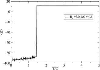
We recognize these two cases simply by detailed inspection of the curves. In the case of continuous phase transitions we could always find an intermediate temperature for which the system is thermodynamically stable at an intermediate energy, and this is not the case for the abrupt phase transitions. In the latter case, there is always an energy gap between two phases. We would expect that microcanonical simulations could produce states in between this gap, but this is outside the scope of this work.

In the case of a first-order phase transition, for $T$ above the transition temperature $T_{c}$, the system is completely disordered (see Fig. 4), both in terms of position (agents act like free particles in a gas) and opinion (no clearly marked preference), whereas below $T_{c}$ the agents are spatially clustered and have a single opinion. We could interpret this kind of phase transition as a “social breakdown”, a state of dissociation between beliefs and opinions. Above $T_{c}$ individuals have lost all trace of their personality, their internal beliefs and their interpersonal relations.

Note that the $E(T)$ curve is flat above $T_{c}$, which is expected because we have no kinetic degrees of freedom in the Hamiltonian, so there is an upper limit to the amount of energy that can be stored in the system. In social terms this means that, under this regime, after the transition individuals immediately reach their upper limit for dissatisfaction.

Figure 3: Internal energy as a function of temperature, for a case in which a second-order phase transition is observed. The values of the parameters are $\rho=0.005$ and $J/C=0.3$.

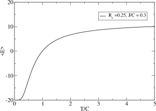
In the case of a second-order phase transition, the system is always spatially disordered (see Fig. 5), because the interaction $J$ that tends to bind them is much weaker than the internal consequence $C$. As the temperature increases, the individuals gradually lose their internal consequence not as a collective, but one by one. In this regime, the social system demonstrates a tolerance to the diversity of opinions and the “social breakdown” is softened.

Figure 4: Probabilities $P_{R}$, $P_{J}$, $P_{C}$ and the decision parameter $M$ as a function of temperature, for the first-order phase transition at $\rho=0.005$ and $J/C=0.3$.

Figure 5: Probabilities $P_{R}$, $P_{J}$ and $P_{C}$ and the decision parameter $M$ as a function of temperature, for the second-order phase transition at $\rho=0.06$ and $J/C=0.6$.

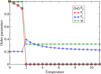
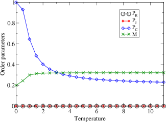
Fig. 6 shows the transition temperature $\tau_{c}=T_{c}/C$ for different values of $J/C$ and $\rho$, presenting both first-order and second-order phase transitions. There is a critical value $C/J=\kappa$, such that for $C>\kappa J$ the transition is second-order, and for $C\leq\kappa J$ the transition is first-order. Fig. 7 shows an estimation of $\kappa$ as a function of the interaction radius $\rho$.

Figure 6: Reduced transition temperature $\tau_{c}=T_{c}/C$ as a function of $\gamma=J/C$ for different values of $\rho$. Curves marked with (*) in the legend are second-order phase transitions.

Figure 7: The critical value of $C/J$, $\kappa$, as a function of $\rho=R_{c}/L$.

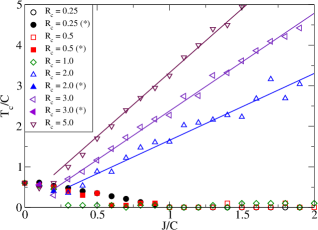
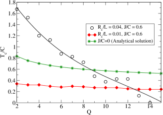
Fig. 8 shows the dependence of the transition temperature with increasing $Q$, the number of possible beliefs or opinions. As expected, $Q$ contributes to the entropy associated with opinions and thus decreases the transition temperature. This can be understood as revealing the following fact: diversity of choices always tends to quicken the onset of the breaking of uniformity, regardless of whether social interaction or personal beliefs are more prevalent.

Figure 8: Reduced transition temperature $\tau_{c}$ as a function of $Q$. Open circles correspond to first-order phase transitions, filled diamonds to second-order. Stars correspond to equation 19.

V Discussion

We have found that the minimum noticeable level of internal consequence $C$ is given by $\kappa J$, a fact which we interpret as follows: the consequence of an individual must overcome a critical value, corresponding to the amount of “opposing” individuals surrounding him/her needed to change his/her own opinion.

When the level of internal consequence falls below this critical value, the individuals have effectively a null internal consequence. In this case, they will either “follow the masses” (at low temperatures) or “follow no one” (at high temperatures). The transition between these two phases is abrupt, first-order, which means there is no state of coexistence, no state where some people are “mass-followers” and some are not. We can imagine this catastrophic change as the dominance of random behavior in agents, where suddenly the whole population loses empathy (connection with others) and rationality (they start disregarding their own internal beliefs).

On the other hand, when $C$ overcomes this critical value, we begin to see continuous, second-order phase transitions. The presence of continuous transitions reveals a system undergoing a smooth change in state (from a fully convinced population at low temperatures to fully undecided individuals at high temperatures). Thus, when $C$ has a greater influence over $J$, the agents’ behavior tends to be governed mostly by their own beliefs instead of the influence (or “social pressure”) exerted by close people. This causes the individual opinion to persist, and therefore, we can argue that each agent is reasonably in agreement with his vision of the world. In thermodynamical terms, this means that the internal energy gradually increases as the imposed temperature increases (the system has a finite, positive heat capacity at all energies).

VI Conclusions

We have proposed a Hamiltonian model, deduced from maximum entropy statistical inference, for a society where individuals can be described only by a personal, internal opinion (or belief) and an external opinion (or behavior). Each individual interacts with others in his/her immediate surroundings and can alter his/her own behavior as a function of the social group he/she belongs to. Our model produces several kinds of agent distributions, which we qualitatively associate with real-life organizations and social phenomena. It is important to note that the derivation of our model relies only on known values for the probabilities $P(S_{i}=B_{i}|H)$ and $P(S_{i}=S_{j}|(r_{ij}<R_{c})\wedge H)$, which can be measured directly in a real-life social setting. The associated parameters $J$, $C$, $R$ or the temperature can be inferred from these probabilities (Eqs. 8, 9, 10 and 11).

Based on our numerical results, we conclude that for an homogeneous society there is a particular “critical” line in parameter space, namely $C=\kappa J$, defining a lower limit for measurable consequence, below which the internal belief is completely forgotten and any given individual only acts as a function of others.