Transverse Momentum Distributions at the LHC and Tsallis Thermodynamics.

Abstract

An overview is presented of transverse momentum distributions of particles at the LHC using the Tsallis distribution. The use of a thermodynamically consistent form of this distribution leads to an excellent description of charged and identified particles. The values of the Tsallis parameter $q$ are truly remarkably consistent.

1 Introduction

It is by now standard to parameterize transverse momentum distributions with functions having a power law behaviour at high momenta. This has been done by the STAR [1] and PHENIX [2] collaborations at RHIC and by the ALICE [3], ATLAS [4] and CMS [5] collaborations at the LHC. In this talk we would like to pursue the use of the Tsallis distribution to describe transverse momentum distributions at the highest beam energies.
In the framework of Tsallis statistics [6, 7, 8, 9, 10] the entropy $S$, the particle number, $N$, the energy density $\epsilon$ and the pressure $P$ are given by corresponding integrals over the Tsallis distribution:

$$f=\left[1+(q-1)\frac{E-\mu}{T}\right]^{-\frac{1}{q-1}}.$$ (1)

It can be shown (see e.g. [10]) that the relevant thermodynamic quantities are given by:

$$S = -gV\int\frac{d^{3}p}{(2\pi)^{3}}\left[f^{q}\ln_{q}f-f\right],$$ (2)

$$N = gV\int\frac{d^{3}p}{(2\pi)^{3}}f^{q},$$ (3)

$$\epsilon = g\int\frac{d^{3}p}{(2\pi)^{3}}Ef^{q},$$ (4)

$$P = g\int\frac{d^{3}p}{(2\pi)^{3}}\frac{p^{2}}{3E}f^{q}.$$ (5)

where $T$ and $\mu$ are the temperature and the chemical potential, $V$ is the volume and $g$ is the degeneracy factor. We have used the short-hand notation

$$\ln_{q}(x)\equiv\frac{x^{1-q}-1}{1-q},$$ (6)

often referred to as q-logarithm. It is straightforward to show that the relation

$$\epsilon+P=Ts+\mu n$$ (7)

(where $n,s,\epsilon$ refer to the densities of the corresponding quantities) is satisfied. The first law of thermodynamics gives rise to the following differential relations:

$$d\epsilon=Tds+\mu dn,$$ (8)

$$dP=sdT+nd\mu.$$ (9)

Since these are total differentials, thermodynamic consistency requires the following Maxwell relations to be satisfied:

$$T = \left.\frac{\partial\epsilon}{\partial s}\right|_{n},$$ (10)

$$\mu = \left.\frac{\partial\epsilon}{\partial n}\right|_{s},$$ (11)

$$N = V\left.\frac{\partial P}{\partial\mu}\right|_{T},$$ (12)

$$S = V\left.\frac{\partial P}{\partial T}\right|_{\mu}.$$ (13)

This is indeed the case, e.g. for Eq. (12) this follows from

$$\left.\frac{\partial P}{\partial\mu}\right|_{T} = -g\int\frac{d^{3}p}{(2\pi)^{3}}\frac{p^{2}}{3}\frac{d}{EdE}\left[1+(q-1)\frac{E-\mu}{T}\right]^{-\frac{q}{q-1}}$$

$$= -g\int\frac{d^{3}p}{(2\pi)^{3}}\frac{p^{2}}{3}\frac{d}{pdp}\left[1+(q-1)\frac{E-\mu}{T}\right]^{-\frac{q}{q-1}}$$

$$= g\int\frac{d\cos\theta d\phi dp}{(2\pi)^{3}}\left[1+(q-1)\frac{E-\mu}{T}\right]^{-\frac{q}{q-1}}\frac{d}{dp}\frac{p^{3}}{3}$$

$$= n$$

after an integration by parts and using $p~{}dp=E~{}dE$.
Following from Eq. (3), the momentum distribution is given by:

$$\frac{d^{3}N}{d^{3}p}=\frac{gV}{(2\pi)^{3}}\left[1+(q-1)\frac{E-\mu}{T}\right]^{-q/(q-1)},$$ (14)

or, expressed in terms of transverse momentum, $p_{T}$, the transverse mass, $m_{T}\equiv\sqrt{p_{T}^{2}+m^{2}}$, and the rapidity $y$

$$\frac{d^{2}N}{dp_{T}~{}dy}=gV\frac{p_{T}m_{T}\cosh y}{(2\pi)^{2}}\left[1+(q-1)\frac{m_{T}\cosh y-\mu}{T}\right]^{-q/(q-1)}.$$ (15)

At mid-rapidity, $y=0$, and for zero chemical potential, as is relevant at the LHC, this reduces to

$$\left.\frac{d^{2}N}{dp_{T}~{}dy}\right|_{y=0}=gV\frac{p_{T}m_{T}}{(2\pi)^{2}}\left[1+(q-1)\frac{m_{T}}{T}\right]^{-q/(q-1)}.$$ (16)

In the limit where the parameter $q$ goes to 1 it is well-known that this reduces to the standard Boltzmann distribution:

$$\lim_{q\rightarrow 1}\frac{d^{2}N}{dp_{T}~{}dy}=gV\frac{p_{T}m_{T}\cosh y}{(2\pi)^{2}}\exp\left(-\frac{m_{T}\cosh y-\mu}{T}\right).$$ (17)

The parameterization given in Eq. (15) is close to the one used by various collaborations [1, 2, 3, 4, 5]:

$$\frac{d^{2}N}{dp_{T}\,dy}=p_{T}\frac{dN}{dy}\frac{(n-1)(n-2)}{nC(nC+m_{0}(n-2))}\left[1+\frac{m_{T}-m_{0}}{nC}\right]^{-n},$$ (18)

where $n$ and $C$ are fit parameters. This corresponds to substituting [19]

$$n\rightarrow\frac{q}{q-1},$$ (19)

and

$$nC\rightarrow\frac{T+m_{0}(q-1)}{q-1}.$$ (20)

After this substitution Eq. (18) becomes

$$\frac{d^{2}N}{dp_{T}\,dy}= p_{T}\frac{{\rm d}N}{{\rm d}y}\frac{(n-1)(n-2)}{nC(nC+m_{0}(n-2))}$$ (21)

$$\left[\frac{T}{T+m_{0}(q-1)}\right]^{-q/(q-1)}$$

$$\left[1+(q-1)\frac{m_{T}}{T}\right]^{-q/(q-1)}.$$

At mid-rapidity $y=0$ and zero chemical potential, this has the same dependence on the transverse momentum as Eq. (16) apart from an additional factor $m_{T}$ on the right-hand side of Eq. (16). However, the inclusion of the rest mass in the substitution Eq. (20) is not in agreement with the Tsallis distribution as it breaks $m_{T}$ scaling which is present in Eq. (16) but not in Eq. (18). The inclusion of the factor $m_{T}$ leads to a more consistent interpretation of the variables $q$ and $T$.
A very good description of transverse momenta distributions at RHIC has been obtained in Refs [11, 12] on the basis of a coalescence model where the Tsallis distribution is used for quarks. Tsallis fits have also been considered in Ref. [13, 14, 15] but with a different power law leading to smaller values of the Tsallis parameter $q$.
Interesting results were obtained in Refs. [16, 17] where spectra for identified particles were analyzed and the resulting values for the parameters $q$ and $T$ were considered.

2 Details of Transverse Momentum Distributions

The transverse momentum distributions of identified particles, as obtained by the ALICE collaboration at 900 GeV in $p-p$ collisions, are shown in Figure 1. The fit for positive pions was made using

$$\left.\frac{d^{2}N}{dp_{T}~{}dy}\right|_{y=0}=V\frac{p_{T}\sqrt{p_{T}^{2}+m_{\pi}^{2}}}{(2\pi)^{2}}\left[1+(q-1)\frac{\sqrt{p_{T}^{2}+m_{\pi}^{2}}}{T}\right]^{-q/(q-1)}.$$ (22)

with $q$, $T$ and $V$ as free parameters.

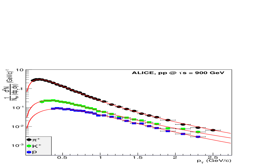
Figure 1: Fits to transverse momentum distributions of positive particles [3] using the Tsallis distribution.

In Figure 2 we show fits to the transverse momentum distributions of strange particles obtained by the ALICE collaboration [3] in $p-p$ collisions at 900 GeV.
Similarly we show fits to the transverse momentum distributions obtained by the CMS collaboration [5] in Figure 4 and by the ATLAS collaboration in Figure 6.
The transverse momentum distributions of charged particles were fitted using a sum of three Tsallis distributions, the first one for $\pi^{+}$, the second one for $K^{+}$ and the third one for protons $p$. The relative weights between these were determined by the corresponding degeneracy factors, i.e. 1 for for $\pi^{+}$ and $K^{+}$ and 2 for protons. The fit was taken at mid-rapidity and for $\mu=0$ using the following expression was used

$$\left.\frac{1}{2\pi p_{T}}\frac{d^{2}N(\mathrm{charged\ particles})}{dp_{T}dy}\right|_{y=0}=\frac{2V}{(2\pi)^{3}}\sum\limits_{i=1}^{3}g_{i}m_{T,i}\left[1+(q-1)\frac{m_{T,i}}{T}\right]^{-\frac{q}{q-1}},$$ (23)

where $i=(\pi^{+},K^{+},p)$ and $g_{\pi^{+}}=1$, $g_{K^{+}}=1$ and $g_{p}=2$. The factor $2$ in front of the right hand side of this equation takes into account the contributions of the antiparticles $(\pi^{-},K^{-},\bar{p})$.

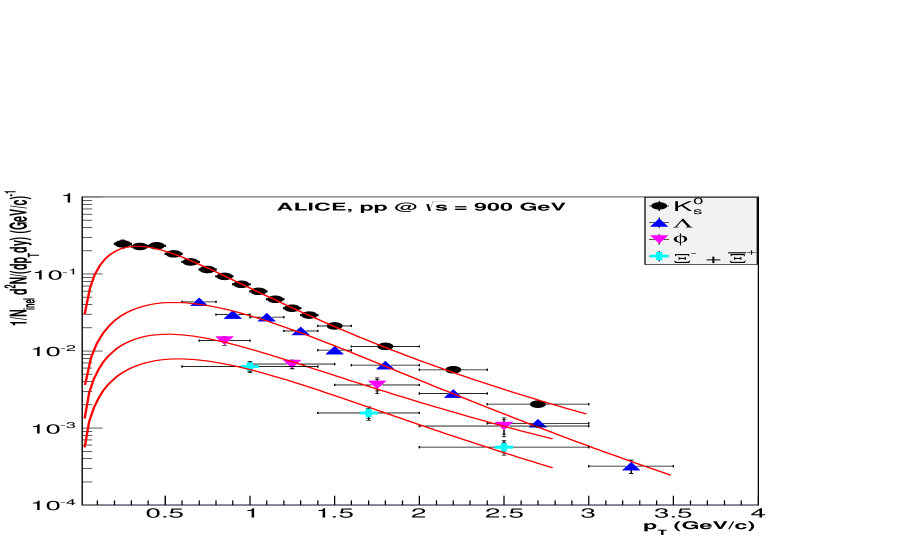
Figure 2: Fits to transverse momentum distributions of strange particles [3] using the Tsallis distribution.

The Tsallis distribution also describes the transverse momentum distributions of charged particles in $p-Pb$ collisions in all pseudorapidity intervals as shown in Figure 4.

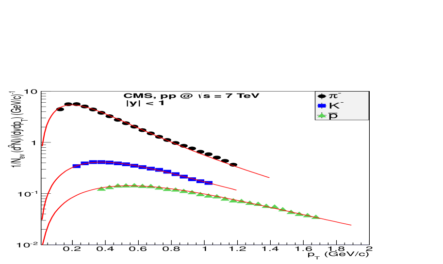
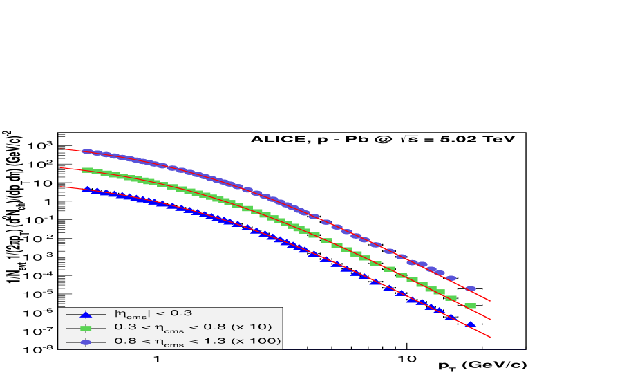
Figure 3: Fits to transverse momentum distributions of negatively charged particles [5] using the Tsallis distribution.

Figure 4: Fits to transverse momentum distributions in $p-Pb$ collisions obtained by the ALICE collaboration  [3] using the Tsallis distribution.

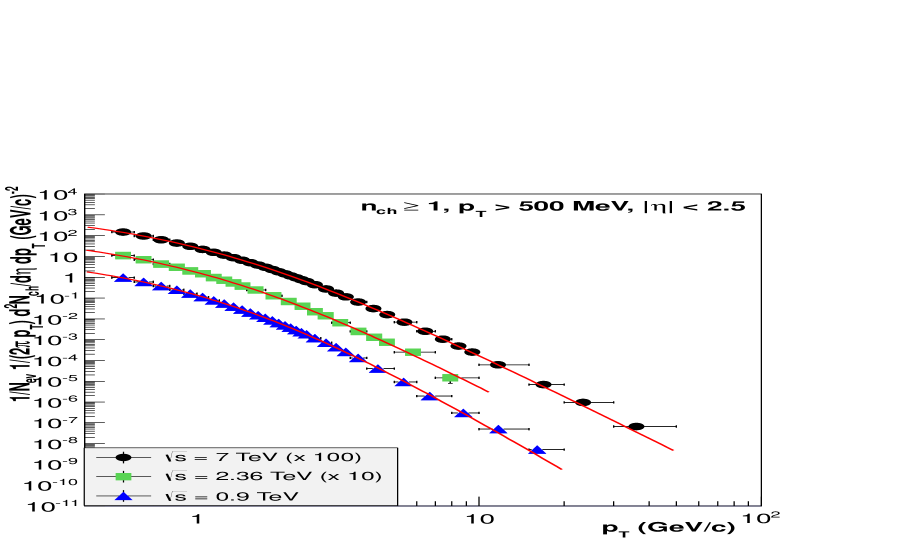
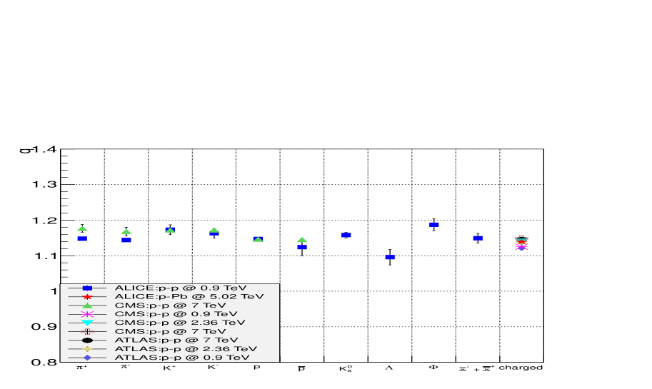
Figure 5: Fits using the Tsallis distribution to transverse momentum distributions of charged particles measured by the ATLAS collaboration [4] in $p-p$ collisions for three different beam energies.

Figure 6: Values of the Tsallis parameter $q$ obtained from fits to transverse momentum spectra described in the text.

3 Summary of Results

The Tsallis distribution described here in Eq. (16) leads to excellent fits to the transverse momentum distributions in high energy $p-p$ and $p-Pb$ collisions. The values obtained for the Tsallis parameter $q$ are truly remarkably consistent, a feature which does not become apparent when using the parametrization of Eq. (18).

References

- [1] B. I. Abelev et al. (STAR Collaboration), Phys. Rev. C 75, 064901 (2007).
- [2] A. Adare et al. (PHENIX Collaboration), Phys. Rev. C 83, 052004, (2010); Phys. Rev. C 83, 064903 (2011).
- [3] ALICE Collaboration, Eur. Phys. J. C 71 1594 (2011); Eur. Phys. J. C 71 1655 (2011); Phys. Lett. B 693 (2010) 53; Phys. Rev. Lett. 110 (2013) 082302.
- [4] ATLAS Collaboration, New J. Phys. 13 (2011) 053033.
- [5] CMS Collaboration, Phys. Rev. Lett. 105 (2010) 022002; Eur. Phys. J. C 72 (2012) 2164.
- [6] C. Tsallis, J. Statist. Phys. 52, 479 (1988).
- [7] T.Biró, G. Purcsel, K. Ürmössy, Eur. Phys. J. A 40 (2009) 325.
- [8] J. M. Conroy, H. G. Miller, A. R. Plastino, Phys. Lett. A 374, 4581 (2010).
- [9] J. Cleymans and D. Worku, J. Phys. G 39 (2012) 025006.
- [10] J. Cleymans and D. Worku, Eur. Phys. J. A 48 (2012) 160.
- [11] K. Ürmössy, T.S. Biró, Phys. Lett. B 689 (2010) 14.
- [12] K. Ürmössy, T.S. Biró, J. Phys. G 36 (2009) 064044.
- [13] Cheuk-Yin Wong, G. Wilk, Acta Physica Polonica, 43 (2012) 2047.
- [14] T. Wibig, J. Phys. G: Nucl. Part. Phys. 37 115009 (2010).
- [15] T. Wibig, I. Kurp, JHEP 0312 039 (2003).
- [16] L. Marques, E.Andrade-II, A. Deppman, arXiv:1210.1725[hep-ph]
- [17] I. Sena, A. Deppman, Eur. Phys. J. A 49 (2013) 17; arXiv:1209.2367[hep-ph]
- [18] K. Ürmössy, arXiv:1212.0260[hep-ph].
- [19] J. Cleymans, G.I. Lykasov, A.S. Parvan, A.S. Sorin, O.V. Teryaev, D. Worku Phys. Lett. B 723 (2013) 351. [arXiv:1104.0620 [hep-ph]].