Nuclear-size self-energy and vacuum-polarization corrections to the bound-electron $\bm{g}$ factor

Abstract

The finite nuclear-size effect on the leading bound-electron $g$ factor and the one-loop QED corrections to the bound-electron $g$ factor is investigated for the ground state of hydrogen-like ions. The calculation is performed to all orders in the nuclear binding strength parameter $Z\alpha$ (where $Z$ is the nuclear charge and $\alpha$ is the fine structure constant) and for the Fermi model of the nuclear charge distribution. In the result, theoretical predictions for the isotope shift of the $1s$ bound-electron $g$ factor are obtained, which can be used for the determination of the difference of nuclear charge radii from experimental values of the bound-electron $g$ factors for different isotopes.

Significant progress has been achieved during the last two decades in the experimental determination of the bound-electron $g$ factor in hydrogen-like (and lithium-like) ions [1, 2, 3, 4, 5]. The current experimental precision is on the level of few parts in $10^{-11}$ and is likely to be improved further in the future. Comparison between the experimental and theoretical results constituted a highly sensitive test of bound-state QED theory [6, 7, 8] and led to an accurate determination of the electron mass [9, 10]. In future, such experiments can also provide us with a new method of determination of other important parameters, in particular, the fine-structure constant [11] and nuclear magnetic moments [12].

In the present work, we investigate one of the possibilities opened by the high-precision $g$ factor experiments, namely, a possibility to determine the nuclear charge radius or the difference of the nuclear charge radii of two isotopes. A proof-of-the-principle determination of the charge radius of ²⁸Si has already been reported in the recent $g$-factor measurement [4]. The nuclear charge distribution effect will play a much more significant role when the planned extension of the $g$-factor measurements to higher-$Z$ systems [13] takes place.

At the present level of theory, the direct determination of the nuclear charge radius is restricted by the theoretical uncertainty due to the two-loop QED effects [7, 8, 14]. In order to avoid this restriction, it might be advantageous to study the isotopic difference of the bound-electron $g$ factor values. Theoretical description of the isotope shift of the $g$ factors is much simpler than that of the $g$ factor itself, as many corrections (in particular, the dominant part of the two-loop QED effects) do not depend on nuclear properties and cancel in the difference. The first experimental determination of the isotopic shift of the bound-electron $g$ factor is currently underway for a calcium ion [13].

The goal of the present work is to perform a detailed investigation of the finite nuclear-size effect on the leading bound-electron $g$ factor and on the one-loop QED corrections to the $g$ factor. The results obtained, combined with the previously reported data on the nuclear recoil correction, allow one to deduce accurate values for the nuclear-dependent part of the $1s$ bound-electron $g$ factor and, therefore, the isotope shift of the $g$ factor.

The remaining paper is organized as follows. In the next section, we discuss the nuclear-size correction to the leading-order bound-electron $g$ factor. In Sec. 2, we calculate the nuclear-size effect on the self-energy and vacuum-polarization corrections to the $g$ factor. Numerical results and experimental consequences are summarized and discussed in Sec. 3. The relativistic units ($\hbar=c=1$) are used throughout the paper.

1 Nuclear-size correction to the leading-order $\bm{g}$ factor

We start with the nuclear-size correction to the relativistic (Breit) value of the bound-electron $g$ factor, defined by the difference

$$\delta g_{\rm N}=g_{\rm ext}^{(0)}-g_{\rm pnt}^{(0)}\,,$$ (1)

where $g_{\rm ext}^{(0)}$ and $g_{\rm pnt}^{(0)}$ are the leading-order bound-electron $g$ factor values evaluated with the extended and the point nuclear models, respectively. For the point nucleus, the well-known analytical result for the $1s$ state reads

$$g_{\rm pnt}^{(0)}=\frac{2}{3}\left[1+2\,\sqrt{1-(Z\alpha)^{2}}\right]\,,$$ (2)

whereas for the extended nucleus the $g$ factor value is given (for the $1s$ state) by the integral

$$g_{\rm ext}^{(0)}=-\frac{8}{3}\,\int_{0}^{\infty}dr\,r^{3}\,g_{a}(r)\,f_{a}(r)\,,$$ (3)

where $g_{a}$ and $f_{a}$ are the upper and lower radial components of the (extended-nucleus) reference-state wave function.

The nuclear-size correction $\delta g_{\rm N}$ can be readily evaluated numerically [15, 16]. For light ions, it can be also obtained analytically by using the expansion in the nuclear binding strength parameter $Z\alpha$ [17, 18]. In Ref. [19], a simple approximate relation was established between the nuclear-size corrections to the $g$ factor and to the binding energy. For the $1s$ state, it reads

$$\delta g_{\rm N}=\frac{4}{3}\,(2\gamma+1)\,\frac{\delta E_{\rm N}}{m}\,,$$ (4)

where $\delta E_{\rm N}$ is the leading-order nuclear-size correction to the Dirac energy and $\gamma=\sqrt{1-(Z\alpha)^{2}}$. The relation (4) goes beyond the $Z\alpha$ expansion and holds with good accuracy in the whole region of the nuclear charge numbers $Z$.

In Table 1, we present our numerical results for the nuclear-size correction $\delta g_{\rm N}$ to the $1s$ bound-electron $g$ factor. The results are parameterized in terms of the dimensionless function $G_{\rm N}(Z,R)$ defined as

$$\delta g_{\rm N}=\frac{8}{3}\,(Z\alpha)^{4}\,\left(\frac{R}{\lambda_{C}}\right)^{2\gamma}\,G_{\rm N}\,,$$ (5)

where $\lambda_{C}=\hbar/mc$, and $R\equiv\langle r^{2}\rangle^{1/2}$ is the root-mean-square (rms) radius of the nuclear-charge distribution. The prefactor before $G_{\rm N}$ in Eq. (5) is consistent with the leading term of the $Z\alpha$ expansion of $\delta g_{\rm N}$ [17], $(8/3)(Z\alpha)^{4}(R/\lambda_{C})^{2}$, so that $G_{\rm N}$ is unity in the nonrelativistic limit. The exponent of $R$ in Eq. (5) follows from Eq. (4) and the relativistic result for the nuclear-size correction to the energy obtained in Ref. [20].

The numerical values of the function $G_{N}$ are presented in the third column of Table 1. The results are obtained with the standard two-parameter Fermi model for the nuclear charge distribution (with the standard choice of the thickness parameter $t=2.3$ fm). Nuclear rms radii used in the calculation are listed in the second column of the table. They were taken from Ref. [21], with the only exception of $Z=92$ for which we used the value from Ref. [22].

We observe that the function $G_{\rm N}$ stays remarkably close to unity in the whole range of $Z$. It might be noted that such smooth behavior of $G_{\rm N}$ is a consequence of the correct relativistic exponent of $R$ in Eq. (5). If we used $R^{2}$ instead of $R^{2\gamma}$ in Eq. (5), we would get a much more rapidly varying function. Namely, $(R/\lambda_{C})^{2\gamma-2}\approx 14$ for $Z=100$, so $G_{\rm N}(Z=100)$ would have been 14 times larger within the $R^{2}$ parametrization.

Having accurate numerical results for $\delta g_{N}$, it might be interesting to check how well the approximate relation (4) holds. Our calculation shows that this relation is accurate to about 1% in the high-$Z$ region and better than that in the low-$Z$ region. Namely, with the numerical results for $\delta E_{\rm N}$ from Ref. [23], Eq. (4) yields $G_{\rm N}(Z=100)=1.125$, $G_{\rm N}(Z=82)=1.213$, and $G_{\rm N}(Z=40)=1.119$, which can be compared with the exact numerical results in the third column of Table 1.

In the fourth column of Table 1, we present differences of the results for $G_{N}$ obtained with the Fermi and the homogeneously charged nuclear models. This difference can be considered as an estimate of the model dependence of the calculational results for the finite nuclear-size correction. We observe that the model dependence of the results is rather weak, ranging from $0.03\%$ in the low-$Z$ region to $0.2\%$ in the high-$Z$ region.

The leading dependence of the nuclear-size correction on the nuclear radius is factorized out by the prefactor $R^{2\gamma}$ in Eq. (5). Still, the function $G_{N}$ depends on $R$, albeit weakly. In order to estimate its $R$ dependence, in the last column of Table 1 we list the results for the derivative $G^{\prime}_{\rm N}(R)=dG_{\rm N}(R)/dR$. We observe that the derivative $G^{\prime}(R)$ is small and scales almost linearly with $Z$.

Numerical data for $G_{\rm N}$ and $G^{\prime}_{\rm N}$ listed in Table 1 allow one to obtain accurate results for the nuclear-size correction to the isotope shift of the $g$ factor. E.g., the difference of the nuclear-size corrections for ²⁰⁸Pb (with $R=5.5010$ fm) and ²⁰⁴Pb (with $R=5.4794$ fm) calculated by using the values of $G_{\rm N}$ and $G^{\prime}_{\rm N}$ listed in Table 1 is $2.8078\times 10^{-6}$, which agrees to all digits with the direct numerical evaluation. The corresponding result calculated without $G^{\prime}_{\rm N}$ ($2.846\times 10^{-6}$) is much less accurate.

Numerical results for $G^{\prime}_{\rm N}$ can also be used for estimating the nuclear deformation effects on the bound-electron $g$ factor. It was demonstrated [24] that the leading quadrupole and hexadecapole nuclear deformation effects to the $g$ factor can be parameterized in terms of shifts of the rms radius. In particular, using Eq. (11) of Ref. [24] one can easily determine the correction to the rms radius due to the quadrupole $\beta_{2}$ and hexadecapole $\beta_{4}$ nuclear deformation parameters and then, using the numerical values for $G^{\prime}_{\rm N}$ from Table 1, obtain the corresponding corrections to the $g$ factor.

Table 1: Leading-order nuclear-size correction to the $1s$ bound-electron $g$ factor. Notations are as follows: $R$ is the nuclear-charge root-mean-square radius (in fermi), $G_{\rm N}$ is the nuclear-size correction for the Fermi model of the nuclear charge distribution, $\delta G_{\rm N}$ is the difference between the results obtained with the Fermi and the homogeneously charged sphere models, and $G^{\prime}_{\rm N}$ is the derivative of $G_{\rm N}$ with respect of $R$ (with $R$ being expressed in fermi units).

$Z$	R [fm]	$G_{\rm N}$	$\delta G_{\rm N}$	$G^{\prime}_{\rm N}$ [1/fm]
4	2.5180	$1.002$
6	2.4703	$1.005$
8	2.7013	$1.009$
10	3.0053	$1.013$
12	3.0568	$1.0183$	$-0.0003$
14	3.1223	$1.0237$	$-0.0003$
16	3.2608	$1.0295$	$-0.0004$
18	3.4269	$1.0356$	$-0.0004$	$-0.0005$
20	3.4764	$1.0421$	$-0.0005$	$-0.0006$
24	3.6424	$1.0559$	$-0.0006$	$-0.0007$
30	3.9286	$1.0781$	$-0.0008$	$-0.0010$
32	4.0744	$1.0857$	$-0.0008$	$-0.0011$
36	4.1882	$1.1013$	$-0.0010$	$-0.0013$
40	4.2696	$1.1170$	$-0.0011$	$-0.0014$
44	4.4818	$1.1324$	$-0.0012$	$-0.0017$
48	4.6137	$1.1473$	$-0.0014$	$-0.0019$
50	4.6543	$1.1545$	$-0.0015$	$-0.0020$
54	4.7866	$1.1681$	$-0.0016$	$-0.0023$
58	4.8770	$1.1806$	$-0.0018$	$-0.0025$
60	4.9118	$1.1862$	$-0.0018$	$-0.0027$
64	5.1617	$1.1955$	$-0.0019$	$-0.0031$
68	5.2505	$1.2030$	$-0.0020$	$-0.0034$
70	5.3115	$1.2057$	$-0.0020$	$-0.0036$
74	5.3670	$1.2090$	$-0.0022$	$-0.0039$
78	5.4278	$1.2087$	$-0.0023$	$-0.0043$
80	5.4633	$1.2070$	$-0.0023$	$-0.0045$
82	5.5010	$1.2042$	$-0.0024$	$-0.0048$
83	5.5211	$1.2023$	$-0.0024$	$-0.0049$
88	5.6841	$1.1877$	$-0.0024$	$-0.0055$
90	5.7100	$1.1794$	$-0.0024$	$-0.0057$
92	5.8569	$1.1689$	$-0.0023$	$-0.0060$
100	5.8570	$1.1115$	$-0.0023$	$-0.0068$

2 Nuclear-size QED corrections

Figure 1: Feynman diagrams representing QED corrections to the bound-electron $g$ factor. The self-energy is represented by graphs (a) and (b), the electric-loop vacuum-polarization by graph (c), the magnetic-loop vacuum-polarization by graph (d). Double lines denote an electron propagating in the binding nuclear field, wave lines denote virtual photons, and the wave line terminated by a cross denotes interaction with an external magnetic field.

The nuclear-size QED correction to the bound-electron $g$ factor can be conveniently parameterized in terms of the dimensionless function $G_{\rm NQED}(Z,R)$,

$$\delta g_{\rm NQED}=\delta g_{\rm N}\,\frac{\alpha}{\pi}\,G_{\rm NQED}\,,$$ (6)

where $\delta g_{\rm N}$ is the leading-order nuclear-size correction given by Eq. (5). Such parametrization of the nuclear-size QED effect is similar to the one used for the Lamb shift [25, 23]. The function $G_{\rm NQED}(Z)$ will be divided into several parts,

$$G_{\rm NQED}=G_{\rm NSE}+G_{\rm NVP,el}+G_{\rm NVP,ml}\,,$$ (7)

where $G_{\rm SE}$ is the nuclear-size correction to the self-energy and $G_{\rm NVP,el}$ and $G_{\rm NVP,ml}$ are the nuclear-size corrections to the electric-loop and magnetic-loop vacuum-polarization, correspondingly. The self-energy correction to the bound-electron $g$ factor is represented graphically on Fig. 1 (a) and (b), whereas the electric-loop and magnetic-loop vacuum-polarization corrections are represented by Fig. 1 (c) and (d), correspondingly.

The nuclear-size effect on the QED corrections to the bound-electron $g$ factor was taken into account previously in several studies. Namely, it was included into the self-energy and vacuum-polarization calculations of Refs. [15, 16] and into the self-energy calculation of Ref. [26]. In Ref. [19], an approximate relation was obtained between the nuclear-size corrections to the $g$ factor and to the binding energy. According to that work, the relative values of the nuclear-size vacuum-polarization corrections to the $1s$ $g$-factor and to the $1s$ binding energy are equal (within the leading logarithmic approximation),

$$\frac{\delta g_{\rm NVP}}{\delta g_{\rm N}}\approx\frac{\delta E_{\rm NVP}}{\delta E_{\rm N}}\,,$$ (8)

where $\delta E_{\rm NVP}$ is the nuclear-size vacuum-polarization correction to the energy. In the present work, we calculate the nuclear-size QED correction with a realistic Fermi model of the nuclear charge distribution and achieve higher numerical accuracy than in previous studies.

The nuclear-size correction to the self-energy is calculated as the difference of the self-energy corrections calculated with the extended and the point nuclear models. The general scheme of calculation of the one-loop self-energy correction to the bound-electron $g$ factor was developed and described in detail in the previous studies involving one of us [6, 26]. For the evaluation of the nuclear-size correction to the self-energy reported in the present work, we needed to extended this scheme for the case of the general binding potential. To this end, we employed the numerical approach for the evaluation of the Dirac Green function for the arbitrary spherically symmetric potential (behaving as $\sim 1/r$ for $r\to\infty$) described in Ref. [23].

2.1 Electric-loop vacuum-polarization

The electric-loop vacuum-polarization correction to the bound-electron $g$ factor is represented by Fig. 1(c) and given by the following expression

$$\Delta g_{\rm VP,el}=2\,\langle a|\left[V_{\rm Uehl}+V_{\rm WK}\right]|\delta_{g}a\rangle\,,$$ (9)

where $|a\rangle$ is the reference-state wave function with a fixed momentum projection $\mu=1/2$, $|\delta_{g}a\rangle$ is first-order perturbation of the reference-state wave function by the effective $g$-factor potential $V_{g}=2m\,[\bm{r}\times\bm{\alpha}]_{z}$,

$$|\delta_{g}a\rangle=\sum_{n\neq a}\frac{|n\rangle\langle n|V_{g}|a\rangle}{\varepsilon_{a}-\varepsilon_{n}}\,,$$ (10)

and $V_{\rm Uehl}$ and $V_{\rm WK}$ are the one-loop Uehling and Wichmann-Kroll potentials, respectively. The Uehling potential is given by the well-known expression

$$V_{\rm Uehl}(r) = -Z\alpha\,\frac{2\alpha}{3\pi}\int\limits_{0}^{\infty}dr^{\prime}\;4\pi r^{\prime}\rho(r^{\prime})$$

$$\times\int\limits_{1}^{\infty}dt\;\left(1+\frac{1}{2t^{2}}\right)\frac{\sqrt{t^{2}-1}}{t^{2}}\frac{e^{-2m|r-r^{\prime}|t}-e^{-2m(r+r^{\prime})t}}{4mrt}\,,$$

where $Z\rho(r)$ is the density of the nuclear charge distribution ($\int\rho(r)d{\bf r}=1$). The Wichmann-Kroll potential is given by [27, 28]

$$V_{\rm WK}(r) = \,\frac{2\alpha}{\pi}\,{\rm Re}\,\sum_{\kappa}|\kappa|\,\int_{0}^{\infty}d\omega\,$$ (12)

$$\times\int_{r}^{\infty}dr^{\prime}r^{\prime}\,\left(1-\frac{r^{\prime}}{r}\right)\,{\rm Tr}\,G_{\kappa}^{(2+)}(i\omega,r^{\prime},r^{\prime})\,,$$

where $G_{\kappa}^{(2+)}$ is the Dirac-Coulomb Green function containing two or more interactions with the binding nuclear field and ”Tr” denotes the trace of the matrix.

The nuclear-size effect on the electric-loop vacuum-polarization correction was calculated as the difference of the vacuum-polarization corrections given by Eq. (9) evaluated with the extended and the point nuclear models. Numerical calculation was carried out similarly to that for the nuclear-size vacuum-polarization correction to the Lamb shift in Ref. [23].

2.2 Magnetic-loop vacuum-polarization

The magnetic-loop vacuum-polarization correction to the bound-electron $g$ factor is represented by Fig. 1(d) and given by the following expression

$$\Delta g_{\rm VP,ml}=\langle a|V_{\rm VP,ml}|a\rangle\,,$$ (13)

where $V_{\rm VP,ml}$ is the magnetic-loop vacuum-polarization potential [29],

$$V_{\rm VP,ml}({\bm{x}}) = \ \frac{i\alpha}{2\pi}\int_{-\infty}^{\infty}d\omega\,\int d{\bm{y}}\,d{\bm{z}}\,\frac{\bm{\alpha}}{|{\bm{x}}-{\bm{y}}|}$$ (14)

$$\times{\rm Tr}\biggl{[}\bm{\alpha}\,G(\omega,{\bm{y}},{\bm{z}})\,V_{g}({\bm{z}})\,G(\omega,{\bm{z}},{\bm{y}})$$

$$-\bm{\alpha}\,G^{(0)}(\omega,{\bm{y}},{\bm{z}})\,V_{g}({\bm{z}})\,G^{(0)}(\omega,{\bm{z}},{\bm{y}})\biggr{]}\,.$$

Here, $G(\omega,{\bm{x}}_{1},{\bm{x}}_{2})$ is the Dirac-Coulomb Green function and $G^{(0)}(\omega,{\bm{x}}_{1},{\bm{x}}_{2})$ is the free Dirac Green function. The scalar product between the vectors of the $\bm{\alpha}$ matrices is implicit in Eq. (14). It is assumed that the expectation value of the potential $V_{\rm VP,ml}$ is calculated with the reference-state wave functions with the momentum projection $\mu_{a}=1/2$. Note that magnetic-loop vacuum-polarization potential contains only the Wichmann-Kroll contribution, as the Uehling part vanishes due to symmetry reasons.

After integrating over the angular variables and rotating the contour of the $\omega$ integration, the magnetic-loop vacuum-polarization correction to the $g$ factor can be expressed as (for an $ns$ reference state)

$$\Delta g_{\rm VP,ml} = \frac{\alpha}{\pi}\int_{0}^{\infty}d\omega\,dx\,dy\,dz\,z^{3}\min(x^{3},y^{3})\,$$ (15)

$$\times g_{a}(x)f_{a}(x)\sum_{\kappa_{1}\kappa_{2}}\frac{4}{9}\,(\kappa_{1}+\kappa_{2})^{2}\,\left[C_{1}(-\kappa_{1},\kappa_{2})\right]^{2}\,$$

$$\times\biggl{[}G_{\kappa_{1}}^{11}G_{\kappa_{2}}^{22}+G_{\kappa_{1}}^{22}G_{\kappa_{2}}^{11}+G_{\kappa_{1}}^{12}G_{\kappa_{2}}^{21}+G_{\kappa_{1}}^{21}G_{\kappa_{2}}^{12}$$

$$-\ldots G\to G^{(0)}\ldots\biggr{]}\,,$$

where $G_{\kappa}^{ij}\equiv G_{\kappa}^{ij}(i\omega,y,z)$ is the radial component of the Dirac-Coulomb Green function and the second term in the brackets is obtained from the first one by substituting the Dirac-Coulomb Green function with the free Dirac Green function. The angular coefficient $C_{J}(\kappa_{a},\kappa_{b})$ is given by

$$C_{J}(\kappa_{a},\kappa_{b}) = (-1)^{j_{a}+1/2}\,\sqrt{(2j_{a}+1)(2j_{b}+1)}\,$$ (18)

$$\times\left(\begin{array}[]{ccc}j_{a}&J&j_{b}\\ \frac{1}{2}&0&-\frac{1}{2}\\ \end{array}\right)\frac{1+(-1)^{l_{a}+l_{b}+J}}{2}\,,$$

where $j=|\kappa|-1/2$ and $l=|\kappa+1/2|-1/2$.

Direct numerical calculations of Eqs. (13)-(15) to all orders in $Z\alpha$ have been performed in Refs. [15, 16]. The calculation reported in these studies was seriously complicated by slow convergence of the partial-wave expansion, especially in the low-$Z$ region, which restricted the final numerical accuracy of the obtained results. More recently, it was demonstrated [30] that the dominant part of this correction (induced by the light-by-light scattering diagram) can be obtained in a closed form, without any partial-wave expansion. The corresponding expression reads

$$\Delta g_{\rm VP,ml}({\rm appr}) = -\frac{32}{3}\frac{\alpha(Z\alpha)^{2}}{\pi}\,\int_{0}^{\infty}dq\,F(q)\,$$ (19)

$$\times\int_{0}^{\infty}dr\left(\frac{\sin qr}{qr}-\cos qr\right)\,r\,g_{a}(r)f_{a}(r)\,,$$

where the function $F(q)$ was calculated numerically and tabulated in Ref. [30].

In order to calculate the nuclear-size correction to the magnetic-loop vacuum-polarization correction, we need to calculate Eq. (13) with an extended and point nuclear models and take the difference of the two results. In order to simplify the numerical evaluation, we divide the nuclear-size correction into two parts, the one induced by the nuclear-size effect on the reference-state wave function and the one induced by the nuclear-size effect on the vacuum-polarization potential. Symbolically, we can write this as

$$\Delta g_{\rm NVP,ml} = \int dx\biggl{[}g_{a}^{\rm ext}(x)f^{\rm ext}_{a}(x)-g_{a}^{\rm pnt}(x)f^{\rm pnt}_{a}(x)\biggl{]}\,V_{\rm VP,ml}^{\rm pnt}(x)$$ (20)

$$+\int dx\,g_{a}^{\rm ext}(x)f^{\rm ext}_{a}(x)\,\biggl{[}V_{\rm VP,ml}^{\rm ext}(x)-V_{\rm VP,ml}^{\rm pnt}(x)\biggl{]}\,,$$

where ”ext” and ”pnt” refer to the extended-nucleus and the point-nucleus model, respectively. The partial-wave expansion of the first part converges very slowly, so we used the approximate expression for the point-nucleus effective potential from Eq. (19) to evaluate this term. The second term was calculated directly according to Eq. (15), by taking the difference of the extended-nucleus and point-nucleus Dirac-Coulomb Green function. In this case, the partial-wave expansion converges rapidly; it was sufficient to take into account just the three first terms of the expansion.

3 Results and discussion

Numerical results of our calculations of the nuclear-size QED corrections to the $1s$ bound-electron $g$ factor of hydrogen-like ions are presented in Table 3 and plotted in Fig. 2. Table 3 also presents comparison with the results obtained in the previous studies [16, 26]. Our results allow us also to check the accuracy of the approximate relation (8) between the nuclear-size vacuum-polarization correction to the $g$-factor and the binding energy. Our conclusion is that this relation yields a rather crude approximation. It holds with accuracy of about 5% for $Z\geq 80$ and 10% for $Z\geq 40$.

We observe that the dominant contribution to the nuclear-size QED correction comes from the self-energy and the Uehling part of the vacuum-polarization. These two contributions are of different sign and largely cancel each other. In the low-$Z$ region, the self-energy dominates over the vacuum-polarization, but in the high-$Z$ region both corrections have the same order of magnitude. The resulting nuclear-size QED correction turns out to be rather small in the whole region of the nuclear charges.

Table 2: Nuclear-size QED corrections to the $1s$ bound-electron $g$ factor, expressed in terms of the function $G_{\rm NQED}(Z)$ defined by Eq. (6). Abbreviations are as follows: ”SE” denotes self-energy contribution, ”Ue,el” denotes the Uehling electric-loop vacuum-polarization correction, ”WK,el” stands for the Wichmann-Kroll electric-loop vacuum-polarization correction, and ”VP,ml” denotes the magnetic-loop vacuum-polarization contribution.

$Z$	R [fm]	SE	Ue,el	WK,el	VP,ml	Total
6	2.4703	$-0.760\,(5)$	$0.180$	$-0.011$	$-0.01\,(1)$	$-0.60\,(1)$
8	2.7013	$-0.930\,(4)$	$0.257$	$-0.019$	$-0.01\,(1)$	$-0.70\,(1)$
10	3.0053	$-1.105\,(3)$	$0.340$	$-0.028$	$-0.014\,(9)$	$-0.807\,(9)$
12	3.0568	$-1.280\,(2)$	$0.433$	$-0.040$	$-0.018\,(8)$	$-0.905\,(8)$
14	3.1223	$-1.458\,(2)$	$0.535$	$-0.053$	$-0.019\,(5)$	$-0.996\,(5)$
20	3.4764	$-1.984\,(2)$	$0.872$	$-0.099$	$-0.027\,(2)$	$-1.237\,(3)$
		$-1.98\,^{a}$
24	3.6424	$-2.338\,(2)$	$1.131$	$-0.134$	$-0.032\,(1)$	$-1.372\,(2)$
30	3.9286	$-2.872\,(2)$	$1.560$	$-0.192$	$-0.038\,(1)$	$-1.542\,(2)$
32	4.0744	$-3.050\,(1)$	$1.708$	$-0.211$	$-0.040\,(1)$	$-1.593\,(1)$
40	4.2696	$-3.787\,(1)$	$2.400$	$-0.298$	$-0.049\,(1)$	$-1.733\,(1)$
50	4.6543	$-4.736\,(1)$	$3.377$	$-0.405$	$-0.057\,(1)$	$-1.821\,(1)$
		$-4.75\,^{a}$
54	4.7866	$-5.130\,(1)$	$3.815$	$-0.449$	$-0.060\,(1)$	$-1.823\,(1)$
60	4.9118	$-5.743\,(1)$	$4.544$	$-0.516$	$-0.065\,(1)$	$-1.780\,(1)$
70	5.3115	$-6.794\,(1)$	$5.860$	$-0.616$	$-0.071\,(1)$	$-1.621\,(1)$
80	5.4633	$-7.951\,(1)$	$7.527$	$-0.730\,(1)$	$-0.077\,(1)$	$-1.232\,(1)$
83	5.5211	$-8.315\,(1)$	$8.090$	$-0.765\,(1)$	$-0.078\,(1)$	$-1.068\,(1)$
90	5.7100	$-9.189\,(1)$	$9.528$	$-0.847\,(1)$	$-0.082\,(2)$	$-0.590\,(2)$
		$-9.186\,^{b}$	$9.494\,^{b}$	$-0.843\,^{b}$	$-0.062\,^{b}$
		$-9.17\,^{a}$
92	5.8569	$-9.427\,(1)$	$9.927$	$-0.866\,(1)$	$-0.083\,(2)$	$-0.449\,(2)$
100	5.8570	$-10.578\,(1)$	$12.173$	$-0.992\,(2)$	$-0.086\,(2)$	$0.518\,(3)$

^a Ref. [26], shell nuclear model; ^b Ref. [16], $R=5.802$.

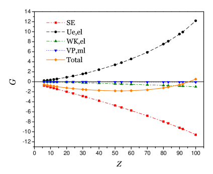
Figure 2: Nuclear-size QED corrections to the $1s$ bound-electron $g$ factor. Notations are the same as in Table 3.

We now turn to the experimental consequences of our calculations. Table 3 presents theoretical results for the nuclear-dependent part of the $1s$ bound-electron $g$ factor and for the isotope shift of the bound-electron $g$ factor for several hydrogen-like ions. The leading-order nuclear-size contribution (labeled as ”N”) and the nuclear-size self-energy (”NSE”) and vacuum-polarization (”NVP”) corrections are taken from Tables 1 and 3. The uncertainty of the leading nuclear-size correction represents the model dependence of the calculation, defined as the difference of the results obtained with the Fermi and the homogeneously charged sphere models.

The data presented in Table 3 for the recoil corrections were taken from the previous studies. The recoil correction of first order in the electron-to-nucleus mass ratio $m/M$ (labeled as ”REC”) was calculated to all orders in $Z\alpha$ in Ref. [31]. The radiative and higher-order recoil corrections are known to the leading order in $Z\alpha$ [32]

$$\Delta g_{\rm REC,QED}=-\frac{\alpha}{\pi}\,\frac{m}{M}\,\frac{(Z\alpha)^{2}}{3}\,,$$ (21)

$$\Delta g_{\rm REC2}=-\left(\frac{m}{M}\right)^{2}\,(Z\alpha)^{2}\,(1+Z)\,.$$ (22)

Apart of the nuclear-size and nuclear-recoil effects, the bound-electron $g$ factor is also influenced by various nuclear-structure effects. Out of those, the nuclear polarization is probably the largest. The correction to the bound-electron $g$ factor due to the nuclear polarization was calculated for several ions in Ref. [33]. Unfortunately, the data presented in that work are not sufficient for our compilation in Table 3. Because of this, we approximate the uncertainty due to the nuclear-polarization effect as 50% of the uncertainty due to the model-dependence of the nuclear-size effect. We observed that for most cases calculated in Ref. [33], the nuclear polarization correction is (crudely) consistent with this simple estimate. In particular, for ${}^{208}_{82}$Pb, our estimate yields $4\times 10^{-7}$, whereas the numerical results of Ref. [33] is $2.2\times 10^{-7}$; for ${}^{84}_{36}$Kr, our estimate yields $1\times 10^{-9}$, to be compared with $1.2\times 10^{-9}$ of Ref. [33].

The final results presented in Table 3 for the nuclear-dependent part of the bound-electron $g$ factor and for the isotope shift have two uncertainties. The first one is the estimation of the model dependence of the nuclear-size correction, whereas the second one is the estimate of the nuclear polarization effect. The errors due to the experimental values of the nuclear radii are not shown explicitly in the table, but they can be easily deduced from the $R$ dependence of the results, see Eq. (5).

We note that the uncertainty of the model dependence of the nuclear-size contribution diminishes significantly in the isotope-shift difference, but not that of the nuclear polarization. The nuclear polarization effect can vary significantly between the isotopes, so one cannot expect a high degree of cancelation in this case. The error due to nuclear polarization dominates in the theoretical isotope shift and currently sets the limit to possible determinations of the difference of the charge radii from the bound-electron $g$ factor measurements.

Summarizing, in the present investigation we calculated the finite nuclear-size effect on the leading bound-electron $g$ factor and on the one-loop QED corrections to the bound-electron $g$ factor in hydrogen-like atoms. The calculation was performed to all orders in the nuclear binding strength parameter $Z\alpha$ and for the Fermi model of the nuclear charge distribution. Combined with the previous calculations of the nuclear recoil effect, our investigation yields theoretical values for the isotope shift of the $1s$ bound-electron $g$ factor that can be used for determination of the isotope differences of the nuclear charge radii from measurements of the bound-electron $g$ factor in hydrogen-like ions.

Acknowledgement

The work presented in the paper was supported by the Alliance Program of the Helmholtz Association (HA216/EMMI). Z.H. acknowledges insightful conversations with Jacek Zatorski and Natalia Oreshkina.

References

Table 3: Nuclear-dependent contributions and the isotope shifts (IS) of the $1s$ bound-electron $g$ factor for several hydrogen-like ions, multiplied by $10^{6}$.

	${}^{40}{\rm Ca}^{19+}$	${}^{44}{\rm Ca}^{19+}$	IS
$R$	$3.4764$	$3.5155$
$m/M\times 10^{5}$	$1.373\,11$	$1.248\,35$
N	$0.113\,029\,(52)$	$0.115\,556\,(52)$	$0.002\,527\,(1)$
NSE	$-0.000\,521$	$-0.000\,533$	$-0.000\,012$
NVP	$0.000\,196$	$0.000\,200$	$0.000\,004$
REC	$0.297\,378$	$0.270\,358$	$-0.027\,020$
REC,QED	$-0.000\,226$	$-0.000\,206$	$0.000\,021$
REC2	$-0.000\,084$	$-0.000\,070$	$0.000\,015$
Total	$0.409\,772\,(52)(26)$	$0.385\,306\,(52)(26)$	$-0.024\,466\,(1)(26)$
	${}^{86}{\rm Kr}^{35+}$	${}^{78}{\rm Kr}^{35+}$	IS
$R$	$4.1836$	$4.2032$
$m/M\times 10^{5}$	$0.6387$	$0.7042$
N	$2.2562\,(20)$	$2.2766\,(20)$	$0.020\,39\,(2)$
NSE	$-0.0179$	$-0.0181$	$-0.000\,16$
NVP	$0.0091$	$0.0092$	$0.000\,08$
REC	$0.4731$	$0.5217$	$0.048\,53$
REC,QED	$-0.0003$	$-0.0004$	$-0.000\,04$
REC2	$-0.0001$	$-0.0001$	$-0.000\,02$
Total	$2.7201\,(20)(10)$	$2.7889\,(20)(10)$	$0.068\,79\,(2)(100)$
	${}^{128}{\rm Xe}^{53+}$	${}^{136}{\rm Xe}^{53+}$	IS
$R$	$4.7755$	$4.7991$
$m/M\times 10^{5}$	$0.4290$	$0.4037$
N	$23.385\,(32)$	$23.597\,(32)$	$0.211\,79\,(45)$
NSE	$-0.277$	$-0.281$	$-0.002\,52$
NVP	$0.180$	$0.181$	$0.001\,63$
REC	$0.808$	$0.761$	$-0.047\,62$
REC,QED	$-0.001$	$0.000$	$0.000\,03$
REC2	$0.000$	$0.000$	$0.000\,02$
Total	$24.094\,(32)(16)$	$24.257\,(32)(16)$	$0.163\,3\,(5)(160)$
	${}^{204}{\rm Pb}^{81+}$	${}^{208}{\rm Pb}^{81+}$	IS
$R$	$5.4794$	$5.5010$
$m/M\times 10^{5}$	$0.2690$	$0.2638$
N	$450.08\,(88)$	$452.89\,(88)$	$2.808\,(11)$
NSE	$-8.57$	$-8.62$	$-0.053$
NVP	$7.39$	$7.43$	$0.046$
REC	$1.76$	$1.72$	$-0.034$
REC,QED	$0.00$	$0.00$	$0.000$
REC2	$0.00$	$0.00$	$0.000$
Total	$450.66\,(88)(44)$	$453.42\,(88)(44)$	$2.767\,(11)(440)$

References

- [1] H. Häffner, T. Beier, N. Hermanspahn, H.-J. Kluge, W. Quint, S. Stahl, J. Verdú, and G. Werth, Phys. Rev. Lett. 85, 5308 (2000).
- [2] J. Verdú, S. Djekić, S. Stahl, T. Valenzuela, M. Vogel, G. Werth, T. Beier, H.-J. Kluge, and W. Quint, Phys. Rev. Lett. 92, 093002 (2004).
- [3] S. Sturm, A. Wagner, B. Schabinger, J. Zatorski, Z. Harman, W. Quint, G. Werth, C. H. Keitel, and K. Blaum, Phys. Rev. Lett. 107, 023002 (2011).
- [4] S. Sturm, A. Wagner, M. Kretzschmar, W. Quint, G. Werth, and K. Blaum, Phys. Rev. A 87, 030501 (2013).
- [5] A. Wagner, S. Sturm, F. Köhler, D. A. Glazov, A. V. Volotka, G. Plunien, W. Quint, G. Werth, V. M. Shabaev, and K. Blaum, Phys. Rev. Lett. 110, 033003 (2013).
- [6] V. A. Yerokhin, P. Indelicato, and V. M. Shabaev, Phys. Rev. Lett. 89, 143001 (2002).
- [7] K. Pachucki, U. D. Jentschura, and V. A. Yerokhin, Phys. Rev. Lett. 93, 150401 (2004), [(E) ibid., 94, 229902 (2005)].
- [8] K. Pachucki, A. Czarnecki, U. D. Jentschura, and V. A. Yerokhin, Phys. Rev. A 72, 022108 (2005).
- [9] T. Beier, H. Häffner, N. Hermanspahn, S. G. Karshenboim, H.-J. Kluge, W. Quint, S. Stahl, J. Verdú, and G. Werth, Phys. Rev. Lett. 88, 011603 (2002).
- [10] P. J. Mohr, B. N. Taylor, and D. B. Newell, Rev. Mod. Phys. 84, 1527 (2012).
- [11] V. M. Shabaev, D. A. Glazov, N. S. Oreshkina, A. V. Volotka, G. Plunien, H.-J. Kluge, and W. Quint, Phys. Rev. Lett. 96, 253002 (2006).
- [12] V. A. Yerokhin, K. Pachucki, Z. Harman, and C. H. Keitel, Phys. Rev. Lett. 107, 043004 (2011).
- [13] K. Blaum, Private communication.
- [14] V. A. Yerokhin and Z. Harman, Phys. Rev. A, in press.
- [15] H. Persson, S. Salomonson, P. Sunnergren, and I. Lindgren, Phys. Rev. A 56, R2499 (1997).
- [16] T. Beier, Phys. Rep. 339, 79 (2000).
- [17] S. G. Karshenboim, Phys. Lett. A 266, 380 (2000).
- [18] D. A. Glazov and V. M. Shabaev, Phys. Lett. A 297, 408 (2002).
- [19] S. G. Karshenboim, R. N. Lee, and A. I. Milstein, Phys. Rev. A 72, 042101 (2005).
- [20] V. M. Shabaev, J. Phys. B 26, 1103 (1993).
- [21] I. Angeli, At. Data Nucl. Data Tables 87, 185 (2004).
- [22] Y. S. Kozhedub, O. V. Andreev, V. M. Shabaev, I. I. Tupitsyn, C. Brandau, C. Kozhuharov, G. Plunien, and T. Stöhlker, Phys. Rev. A 77, 032501 (2008).
- [23] V. A. Yerokhin, Phys. Rev. A 83, 012507 (2011).
- [24] J. Zatorski, N. S. Oreshkina, C. H. Keitel, and Z. Harman, Phys. Rev. Lett. 108, 063005 (2012).
- [25] A. I. Milstein, O. P. Sushkov, and I. S. Terekhov, Phys. Rev. A 69, 022114 (2004).
- [26] V. A. Yerokhin, P. Indelicato, and V. M. Shabaev, Phys. Rev. A 69, 052503 (2004).
- [27] G. Soff and P. Mohr, Phys. Rev. A 38, 5066 (1988).
- [28] N. L. Manakov, A. A. Nekipelov, and A. G. Fainshtein, Zh. Eksp. Teor. Fiz. 95, 1167 (1989), [Sov. Phys. JETP 68, 673 (1989)].
- [29] A. N. Artemyev, V. M. Shabaev, G. Plunien, G. Soff, and V. A. Yerokhin, Phys. Rev. A 63, 062504 (2001).
- [30] R. N. Lee, A. I. Milstein, I. S. Terekhov, and S. G. Karshenboim, Phys. Rev. A 71, 052501 (2005).
- [31] V. M. Shabaev and V. A. Yerokhin, Phys. Rev. Lett. 88, 091801 (2002).
- [32] M. I. Eides and H. Grotch, Ann. Phys. (NY) 260, 191 (1997).
- [33] A. V. Nefiodov, G. Plunien, and G. Soff, Phys. Rev. Lett. 89, 081802 (2002).