Object Detection Using Keygraphs

Abstract

We propose a new framework for object detection based on a generalization of the keypoint correspondence framework. This framework is based on replacing keypoints by keygraphs, i.e. isomorph directed graphs whose vertices are keypoints, in order to explore relative and structural information. Unlike similar works in the literature, we deal directly with graphs in the entire pipeline: we search for graph correspondences instead of searching for individual point correspondences and then building graph correspondences from them afterwards. We also estimate the pose from graph correspondences instead of falling back to point correspondences through a voting table. The contributions of this paper are the proposed framework and an implementation that properly handles its inherent issues of loss of locality and combinatorial explosion, showing its viability for real-time applications. In particular, we introduce the novel concept of keytuples to solve a running time issue. The accuracy of the implementation is shown by results of over 800 experiments with a well-known database of images. The speed is illustrated by real-time tracking with two different cameras in ordinary hardware.

Keywords: Object detection; keypoint correspondences; graph isomorphism; structural pattern recognition.

1 Introduction

Object detection is a well-known problem in computer vision that consists in: given a model representing an object and a scene, decide if there are instances of the object in the scene and, if so, estimate the pose of each instance. Solving this problem is useful for many applications like automatic surveillance, medical analysis, and augmented reality, but particularly challenging due to difficulties like image distortions, background clutter, and partial occlusions.

Among the techniques for object detection available in the literature, methods based on keypoint correspondence have been particularly successful [32, 33, 30, 5, 41]. The outline of such methods consists in detecting interest points in the model and the scene, selecting correspondences between the two sets of points by analyzing the similarity between photometric descriptors, and applying a fitting procedure over those correspondences. This framework is not specific to object detection and has also been used for robot navigation [40], feature tracking [34, 58, 49], stereo matching [34, 36, 57], image retrieval [47], $3$D reconstruction [5] and visual odometry [1].

In this paper, we propose a framework for object detection based on replacing keypoints by keygraphs, i.e. isomorph directed graphs whose vertices are keypoints, in the aforementioned outline. The motivation for this proposal is exploring relative and structural information that an individual point cannot provide. Because keygraphs can be more numerous and complex, such replacement is not straightforward. Two issues must be considered: a possible loss of locality, since large structures might be built, and a possible combinatorial explosion, since large sets might be enumerated. Therefore, in addition to describing the framework itself, we describe an implementation that takes those issues into account.

In a previous work [21], the viability of the keygraph framework has already been proved by an implementation that uses chromaticity values for keygraph description and the Hough transform [2] for pose estimation. Here, in addition to presenting a more complete formalization and a deeper theoretical analysis, we improve such work by using intensity values for keygraph description and the RANSAC algorithm [16] for pose estimation. The former allowed a greater accuracy for gray-level images and the latter allowed a wider range of possible poses. Numerical results from extensive experiments show that our implementation has competitive accuracy and low running time.

This paper is organized as follows. Section 2 presents related works in the literature and specifies how ours differs from them. Section 3 presents an overview of the keygraph framework, which includes formal definitions of keygraph and keygraph correspondence. Section 4 presents the concept of keytuples, which we introduce as a solution for a running time issue. Section 5 presents our implementation of the keygraph detection, based on combinatorial and geometric criteria. Section 6 presents our implementation of the keygraph description, based on Fourier coefficients of intensity profiles. Section 7 presents our implementation of correspondence selection and pose estimation using RANSAC. Section 8 presents experimental results. Finally, Section 9 presents our conclusions and research directions.

2 Related work

Since the proposed keygraph framework is based on the generalization of the original keypoint framework, as shown in Section 3, all work based on keypoint correspondence may be considered related. For a literature revision of such work, we refer to the comparative study of descriptors by Mikolajczyk and Schmid [38], the comparative study of detectors by Mikolajczyk et al. [39], and the survey by Tuytelaars and Mikolajczyk [59].

In particular, the idea of exploring relative and structural information in keypoint correspondence is not new. The seminal paper of Schmid and Mohr [47], for example, already recognized the importance of geometric criteria for correspondence selection. A more recent example is the widely used shape context descriptor [6], originally defined as a histogram of relative point positions. The difference of this paper relies on obtaining the information from graphs with fixed size, while the aforementioned authors consider neighborhoods with variable size.

Besides being seen as a generalization of the keypoint framework, there are alternative interpretations for the contributions of the keygraph framework, and the related literature varies accordingly. One possible interpretation is that we consider a structure of parts instead of individual parts. This idea has been successfully used in statistical approaches for image categorization like the constellation model proposed by Weber et al. [60], the spatial priors proposed by Crandall et al. [13], the multiscale tree proposed by Bouchard and Triggs [7], and the sparse flexible models proposed by Carneiro and Lowe [11]. The approach of Leordeanu et al. [29] is particularly relevant for sharing the generic idea of using descriptors that are individually robust and collectively discriminative. Such idea plays a role in Section 6.

Another, less vague, interpretation is that we use graphs whose vertices are keypoints. We can cite the work of Tang and Tao [54], which consists in applying graph matching procedures [27, 10, 25] over graphs whose vertices are SIFT keypoints [32, 33] for detecting objects, and the work of Sirmacek and Unsalan [51], which consists in applying graph cut procedures also over graphs whose vertices are SIFT keypoints for detecting urban areas in aerial photographs. Those approaches, however, are global: the objective is obtaining a single large graph. Our approach, in contrast, is local: the objective is obtaining multiple small graphs.

Considering such locality, the papers of Tell and Carlsson [55, 56] and Kanazawa and Uemura [24] are closer. The former not only introduced the idea of computing descriptors from intensity profiles of keypoint pairs, which we use in Section 6, but also showed the importance of relative positioning, which we use in Section 5. The latter extended those contributions using triplet vector descriptors and normalized triangular region vectors. The pair correspondences of Tell and Carlsson and the triplet correspondences of Kanazawa and Uemura can be considered precursors of keygraph correspondences, but their usefulness for pose estimation is limited by a voting table that transforms them into an ordinary set of independent keypoint correspondences. The Natural 3D Markers (N3M) proposed by Hinterstoisser et al. [22] do not have this limitation and are perhaps the closest concept to keygraphs currently available in the literature. However, Hinterstoisser et al. do not analyze Natural 3D Markers directly like we do with keygraphs: instead, they select independent keypoint correspondences and verify which N3M correspondences are implied by those.

Structures of keypoints have also been successful in content-based image retrieval, particularly in works based on visual words [53, 44] where descriptors are quantized into a visual vocabulary using clustering. This process is also conceptually related to Section 6: the clustering can be interpreted as simplifying the descriptors, while the structures can be interpreted as an attempt to use collectivity for recovering distinctiveness lost in quantization. Relevant examples are the doublets proposed by Sivic et al. [52], the visual phrases proposed by Yuan et al. [61], the TSR proposed by Punitha and Guru [45], and the $\Delta$-TSR proposed by Hoang et al. [23]. Another successful approach based on introducing a structure to compensate for descriptor limitations is the spatial pyramid matching [28].

3 Overview of the keygraph framework

The following table illustrates the analogy between the existing keypoint framework and the proposed keygraph framework.

keypoint framework	keygraph framework
1 detect model keypoints $\mathcal{P}_{m}$ and scene keypoints $\mathcal{P}_{s}$	1 detect model keypoints $\mathcal{P}_{m}$ and scene keypoints $\mathcal{P}_{s}$
	detect model keygraphs $\mathcal{G}_{m}$ and scene keygraphs $\mathcal{G}_{s}$
2 compute the descriptor of each keypoint	2 compute the descriptors of each keygraph
3 select keypoint correspondences	3 select keygraph correspondences
4 estimate pose using the selected correspondences	4 estimate pose using the selected correspondences

The numbering represents the four steps that both frameworks analogously have: detection, description, selection, and estimation. Keypoint detection is the first task of both frameworks, and the only task that does not require adaptation for the keygraph framework: we can directly use the existing algorithms.

Figure 1 illustrates the sequence of steps defined by the proposed framework. In our implementation, a descriptor is not global with respect to the graph: we compute local descriptors and select correspondences by partwise analysis.

(a)                (b)                 (c)                 (d)                (e)

Figure 1: Illustration of the framework. (a) Model and scene. (b) Detection of keypoints $\mathcal{P}_{m}$ and $\mathcal{P}_{s}$. (c) Detection of keygraphs $\mathcal{G}_{m}$ and $\mathcal{G}_{s}$. (d) Selection of correspondences. (e) Pose estimation.

3.1 Definition of keygraph

As mentioned in Section 1, keygraphs are isomorph directed graphs whose vertices are keypoints. More formally:

• each keygraph is a pair $(\mathcal{V},\mathcal{A})$, where the set of vertices $\mathcal{V}$ is a subset of keypoints and the set of arcs $\mathcal{A}$ is a subset of $\{(v,w)\colon v,w\in\mathcal{V}\textrm{ and }v\not=w\}$;

• for any keygraphs $G_{1}=(\mathcal{V}_{1},\mathcal{A}_{1})$ and $G_{2}=(\mathcal{V}_{2},\mathcal{A}_{2})$, there exists a bijection $\iota\colon\mathcal{V}_{1}\rightarrow\mathcal{V}_{2}$ with arc preservation: $(a,b)\in\mathcal{A}_{1}$ if and only if $(\iota(a),\iota(b))\in\mathcal{A}_{2}$. Such bijection is called an isomorphism from $G_{1}$ to $G_{2}$.

The isomorphism requirement is our proposed solution for the issue of comparability: unlike a pair of points, a pair of graphs can have structural differences and therefore requires structural criteria for deciding whether it is comparable. We propose bijection as a criterion to purposefully avoid mapping multiple model keypoints to a single scene keypoint. This contrasts, for example, with works where super-segmentation graphs are mapped to segmentation graphs [12]: in such works, surjections are more adequate. The criterion of arc preservation, in its turn, avoids mapping an arc to a pair that is not an arc. This ensures the aforementioned partwise analysis: the isomorphism establishes which model vertex should be compared to each scene vertex and which model arc should be compared to each scene arc.

Note that the keygraph framework is a generalization of the keypoint framework: a keypoint can be interpreted as a keygraph with a single vertex, and from a single-vertex graph to another there is always an isomorphism.

3.2 Definition of keygraph correspondence

A keygraph correspondence is a triple $(G_{m},G_{s},\iota)$, where $G_{m}$ is a model keygraph, $G_{s}$ is a scene keygraph, and $\iota$ is an isomorphism from $G_{m}$ to $G_{s}$. Specifying the isomorphism is our proposed solution for the issue of multi-comparability: from one graph to another, more than one isomorphism can exist. Figure 2 shows an example.

(a)                          (b)                                          (c)

Figure 2: Example of multi-comparability. (a) A model keygraph with vertices $a_{m},b_{m},c_{m}$ and a scene keygraph with vertices $a_{s},b_{s},c_{s}$. (b) Visual representation of the three isomorphisms from the model keygraph to the scene keygraph: for each isomorphism $\iota$, a dashed arrow from a model vertex $v$ to a scene vertex $w$ illustrates that $\iota(v)=w$. (c) The same representation, after repositioning the vertices to emphasize arc preservation.

In contrast, a keypoint correspondence is simply a pair $(p_{m},p_{s})$, where $p_{m}$ is a model keypoint and $p_{s}$ is a scene keypoint. Note that a keygraph correspondence $(G_{m},G_{s},\iota)$ implies the set of keypoint correspondences

$$\{(v,\iota(v))\colon v\textrm{ is a vertex of }G_{m}\}$$ (1)

and therefore a set of keygraph correspondences $\Gamma$ implies the set of keypoint correspondences

$$\Pi:=\bigcup_{(G_{m},G_{s},\iota)\in\Gamma}\{(v,\iota(v))\colon v\textrm{ is a vertex of }G_{m}\}$$ (2)

The first implication is particularly relevant for estimating pose using RANSAC, as shown in Section 7, and the second implication is particularly relevant for analyzing our experimental results, as shown in Section 8.

In our implementation, we assume few models and many scenes: this is reasonable for applications such as video tracking and content-based image retrieval. Under this assumption, detecting model keygraphs and computing their respective descriptors once and storing them for subsequent usage is more adequate than repeating such detection and computation for each scene. Therefore, we implement the following asymmetric version of the framework.

1	detect and store model keypoints $\mathcal{P}_{m}$
2	detect and store model keygraphs $\mathcal{G}_{m}$
3	for each $G_{m}$ in $\mathcal{G}_{m}$
4	compute and store the descriptors of $G_{m}$
5	for each scene
6	detect scene keypoints $\mathcal{P}_{s}$
7	detect scene keygraphs $\mathcal{G}_{s}$
8	for each $G_{s}$ in $\mathcal{G}_{s}$
9	compute the descriptors of $G_{s}$
10	for each $G_{m}$ in $\mathcal{G}_{m}$
11	for each isomorphism $\iota$ from $G_{m}$ to $G_{s}$
12	select or reject $(G_{m},G_{s},\iota)$
13	estimate pose using the selected correspondences

We also assume availability of time for this storage: only correspondence selection and pose estimation must be as fast as possible. Such assumption allows us to process the model keygraphs and their respective descriptors to make the correspondence selection faster. This paradigm has been successful in the literature of keypoint correspondence, particularly in works based on indexing structures [32, 33] and machine learning [30, 46].

Therefore, throughout this paper we prioritize exhaustiveness when extracting model data and prioritize speed when extracting scene data. Such paradigm can be summarized as follows:

• sacrifice, for speed, the majority of scene information;

• ensure, with exhaustiveness, that any remaining scene information that can be mapped to model information will be mapped to model information.

This is particularly relevant for keygraph detection, as seen in Section 5, and also relevant in Section 4.

4 Keytuples

Given a set of model keygraphs and a set of scene keygraphs, obtaining correspondences is not straightforward because a bijection from a model graph vertex set to a scene graph vertex set might not be an isomorphism. In Figure 2, for example, the three isomorphisms represent only half of the six possible bijections. This raises an issue:

• on one hand, the exhaustive verification of all bijections is expensive: if the keygraphs have $k$ vertices, there are $k!$ possible bijections;

• on the other hand, an isomorphism to a scene graph cannot be stored when only model graphs are available.

In order to solve this issue, we introduce the concept of keytuples. Let $G=(\mathcal{V},\mathcal{A})$ be a keygraph with $k$ vertices, $(v_{1},\ldots,v_{k})$ be an ordering of $\mathcal{V}$, and $\sigma$ be a $k\times k$ binary matrix. We say $(v_{1},\ldots,v_{k})$ is a keytuple of $G$ with respect to $\sigma$ if

$$\sigma_{ij}=\left\{\begin{array}[]{ll}1&\textrm{ if }(v_{i},v_{j})\textrm{ belongs to }\mathcal{A};\\ 0&\textrm{ otherwise.}\end{array}\right.$$

In other words, $\sigma$ establishes for each $i,j$ whether there is an arc in $G$ from the $i$-th to the $j$-th vertex of the keytuple. In Figure 2, for example, the orderings $(a_{m},b_{m},c_{m}),(c_{m},a_{m},b_{m}),(b_{m},c_{m},a_{m})$ are keytuples of the model graph with respect to

$$\left[\begin{array}[]{ccc}0&1&0\\ 0&0&1\\ 1&0&0\end{array}\right]$$

because this matrix establishes that there are arcs from the first to the second vertex, from the second to the third vertex, and from the third to the first vertex.

From the definition of isomorphism and the definition of keytuple, it is easy to prove the following proposition.

Proposition 1.

Let $G_{m}=(\mathcal{V}_{m},\mathcal{A}_{m}),G_{s}=(\mathcal{V}_{s},\mathcal{A}_{s})$ be keygraphs, $\sigma$ be a matrix, $(w_{1},\ldots,w_{k})$ be a keytuple of $G_{s}$ with respect to $\sigma$, and $\mathcal{T}$ be the set of keytuples of $G_{m}$ with respect to $\sigma$. Then a bijection $\iota\colon\mathcal{V}_{m}\rightarrow\mathcal{V}_{s}$ is an isomorphism from $G_{m}$ to $G_{s}$ if and only if there exists a keytuple $(v_{1},\ldots,v_{k})$ in $\mathcal{T}$ such that $\iota(v_{i})=w_{i}$ for all $i$.

This allows a straightforward procedure for obtaining all isomorphisms from a model keygraph $G_{m}$ to a scene keygraph $G_{s}$ given a matrix $\sigma$:

1. let $\mathcal{T}_{m}$ be the set of all keytuples of $G_{m}$ with respect to $\sigma$;

2. let $(w_{1},\ldots,w_{k})$ be a keytuple of $G_{s}$ with respect to $\sigma$;

3. for each keytuple $(v_{1},\ldots,v_{1})$ in $\mathcal{T}_{m}$, let $\iota$ be the isomorphism from $G_{m}$ to $G_{s}$ such that $\iota(v_{i})=w_{i}$ for all $i$.

Such procedure fits adequately into the paradigm of prioritizing exhaustiveness when extracting model data and prioritizing speed when extracting scene data: Step 1 considers all model keytuples, while Step 2 chooses a single scene keytuple. The proposition ensures the choice can be arbitrary.

Figure 3 shows an example of keytuples and the following outline adapts the asymmetric framework to them.

(a)                                     (b)                             (c)

Figure 3: Continuation of Figure 2 for an example of keytuples. The dashed arrows in illustration (a) are not necessary because the isomorphisms are implied by vertex ordering. Illustration (b) is simpler but redundant because the same scene keytuple is repeated. Illustration (c) emphasizes the asymmetry.

1	detect and store model keypoints $\mathcal{P}_{m}$
2	detect and store model keygraphs $\mathcal{G}_{m}$
3	for each $G_{m}$ in $\mathcal{G}_{m}$
4	compute and store the descriptors of $G_{m}$
5	for each keytuple $(v_{1},\ldots,v_{k})$ of $G_{m}$
6	store $(v_{1},\ldots,v_{k})$ in $\mathcal{T}_{m}$
7	for each scene
8	detect scene keypoints $\mathcal{P}_{s}$
9	detect scene keygraphs $\mathcal{G}_{s}$
10	for each $G_{s}$ in $\mathcal{G}_{s}$
11	compute the descriptors of $G_{s}$
12	let $(w_{1},\ldots,w_{k})$ be a keytuple of $G_{s}$
13	for each keytuple $(v_{1},\ldots,v_{k})$ in $\mathcal{T}_{m}$
14	let $G_{m}$ be the graph in $\mathcal{G}_{m}$ such that $(v_{1},\ldots,v_{k})$ is a keytuple of $G_{s}$
15	let $\iota$ be the isomorphism from $G_{m}$ to $G_{s}$ such that $\iota(v_{i})=w_{i}$ for all $i$
16	select or reject $(G_{m},G_{s},\iota)$
17	estimate pose using the selected correspondences

Note that this adaptation replaced a double loop in keygraphs and isomorphisms by a single loop in keytuples.

5 Keygraph detection

In a previous work [21], the implementation used the Good Features To Track algorithm [49] to detect keypoints, as it provided a good balance between accuracy and speed for the experiments. In this paper, our implementation uses the Hessian-Affine [37, 39] and MSER [36] algorithms. The former is based on extrema of Hessian determinants over multiple scales and the latter is based on extremal regions that are maximally stable. Both are actually covariant region detectors, converted to keypoint detectors by taking the region centroids.

Those detectors were chosen because they provide the best results in the aforementioned comparative study by Mikolajczyk et al. [39]. We decided to use both because neither of them consistently outperforms the other in all experiments of such study. The advantages and disadvantages of each one influenced the experimental results presented in Section 8.

Furthermore, following the paradigm of prioritizing exhaustiveness when extracting model data and prioritizing speed when extracting scene data, we use a subset of the scene keypoints. This subset is obtained by randomly choosing a maximal set of points such that no pair is excessively close according to the Chebyshev distance. More formally: given two keypoints $(x_{1},y_{1})$ and $(x_{2},y_{2})$,

$$\max\{|x_{2}-x_{1}|,|y_{2}-y_{2}|\}$$

cannot be lower than a certain value. In our experiments, the adopted value is $10$ pixels.

The keygraph detector is based on combinatorial and geometric criteria. Most of such criteria is applied to both model graphs and scene graphs, but some of them are applied only to the scene. We start by describing the shared criteria and conclude the section with the criteria specific to the scene.

The combinatorial criterion is the structure of the keygraphs. Figure 4 shows the three structures chosen for our experiments, and the respective matrices chosen for defining keytuples.

$\left[\begin{array}[]{cc}0&1\\ 0&0\end{array}\right]$	$\left[\begin{array}[]{ccc}0&1&0\\ 0&0&1\\ 1&0&0\end{array}\right]$	$\left[\begin{array}[]{cccc}0&1&0&0\\ 0&0&1&0\\ 0&0&0&1\\ 1&0&0&0\end{array}\right]$
(a)	(b)	(c)

Figure 4: The three structures chosen and their respective matrices. (a) Two vertices and the arc from one to the other. (b) Circuit with three vertices. (c) Circuit with four vertices.

Such structures and matrices were chosen because obtaining keytuples from them is straightforward and fast: for the first structure the keytuple is unique, and for the second and third structures a keytuple is always a cyclic permutation of another keytuple. Larger circuits could have been used, but the experimental results of Section 8 suggested that the possible gain in accuracy would not justify the loss in running time.

The geometric criteria, on the other hand, are three. The first criterion is minimum distance: two vertices of a keygraph cannot be excessively close according to the Chebyshev distance. This criterion was chosen because, as shown in Section 6, we compute descriptors from intensity profiles. An intensity profile is the sequence of values of the pixels intersected by the straight line between the two vertices of an arc. Our implementation uses the Bresenham algorithm [9] to obtain those values. Since the length of a profile obtained with such algorithm is the Chebyshev distance between the respective vertices, the criterion avoids short arcs and therefore poor descriptors. In our experiments, we use a minimum distance of $10$ pixels chosen empirically. The same distance is used to sample the scene keypoints.

The second geometric criterion is maximum distance. This criterion was chosen to avoid long arcs and therefore the consequences of loss of locality: short intensity profiles are more robust to perspective transforms and more adequate for non-planar objects. For the model keygraphs, we use a maximum distance of $100$ pixels chosen empirically. For the scene keygraphs, we do not use a maximum distance because in our experiments the instance of the object in the scene can be much larger than the model.

Finally, the third criterion is relative positioning: if the graph is one of the two circuits, its arcs must have clockwise direction. This criterion was chosen because we assume that mirroring is not one of the possible distortions that an instance of the object can suffer in the scene. Under this assumption, mapping a clockwise circuit to a counter-clockwise circuit does not make sense. Deciding whether a circuit is clockwise requires a straightforward and fast cross-product operation.

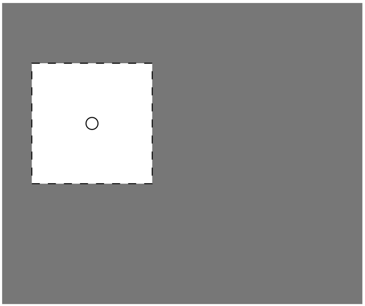
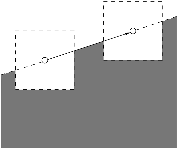
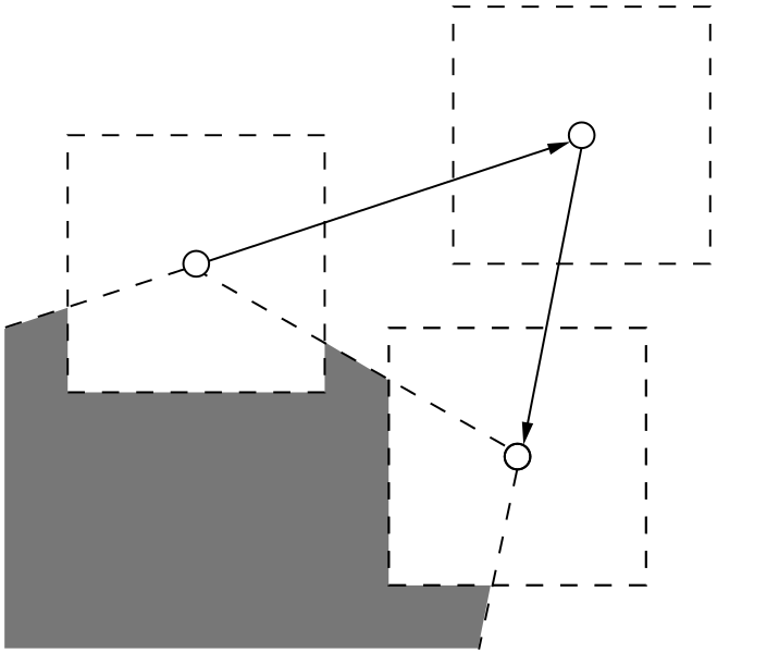
Note that the geometric criteria can alleviate the combinatorial explosion by reducing the number of graphs, as illustrated by Figure 5.

(a)	(b)	(c)

Figure 5: Potential of geometric criteria for reducing the number of keygraphs. Specifically, minimum distance and relative positioning. (a) After choosing the first vertex, the gray set of points that can be the second vertex is limited by minimum distance. (b) After choosing the second one, the set of points that can be the third one is limited by minimum distance and relative positioning. Note that more than half of the Euclidean plane does not belong to the set at this stage. (c) After choosing the third, the set that can be the fourth is limited even further.

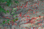
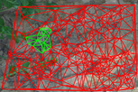
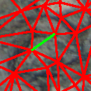
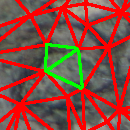
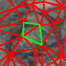
From a theoretical point of view, the aforementioned combinatorial and geometric criteria are enough to keep the number of model keygraphs tractable. Since keygraphs are isomorph, the chosen structures ensure that such number is either $O(n^{2})$, $O(n^{3})$, or $O(n^{4})$, where $n$ is the number of keypoints. In our implementation, we store the descriptors in an indexing structure that allows correspondence selection in expected logarithmic time. Therefore, since $\log kn=k\log n$, correspondence selection is sublinear on the keypoints. A superlinear number of scene keygraphs, however, is not tractable. Therefore, for those keygraphs we choose an additional geometric criterion: they must be obtained from the edges and faces of the Delaunay triangulation [14] of the keypoints. Figure 6 shows an example. Obtaining the first structure from edges and the second structure from faces is straightforward. The third structure can be obtained from internal edges, as illustrated by Figure 7.

(a)	(b)	(c)	(d)

Figure 6: Example of Delaunay triangulation (a) Model. (b) Scene and pose of the instance of the object in the scene. (c) Scene keypoints: points that can be mapped to the model are emphasized. (d) Delaunay triangulation of the keypoints: edges and faces that can be mapped to the model are emphasized.

(a)	(b)	(c)

Figure 7: Obtaining a circuit with four vertices from an internal edge of a Delaunay triangulation. (a) The internal edge. (b) The two faces that share the internal edge. (c) The symmetric difference of the edge sets of the two faces.

Since the Delaunay triangulation is a planar graph, the Euler formula can be used to prove that the number of edges and faces is $O(n)$ [14]. Furthermore, such triangulation can be obtained in $O(n\log n)$ time [17].

Note that for dense keypoint detectors, such as Hessian-Affine, the Delaunay triangulation can have an excessive number of short edges and therefore an excessive reduction on the number of keygraphs. This explains why we sample the scene keypoints according to the minimum distance. Note also that, although the triangulation is not robust to perspective transforms, it does not have to be: we do not care if the entire planar graph can me mapped to the model keygraphs, only if each scene keygraph individually can. Again, we prioritize exhaustiveness when extracting model data and prioritize speed when extracting scene data.

6 Keygraph description

In our implementation, as shown in Section 3, we select correspondences by partwise analysis and the isomorphism establishes which model vertex should be compared to each scene vertex and which model arc should be compared to each scene arc. The descriptor chosen for the vertices is the widely used SIFT descriptor [32, 33], which is based on a weighted histogram of gradient orientations and provides the best results in the comparative study of Mikolajczyk and Schmid [38]. The descriptor chosen for the arcs is based on Fourier coefficients of the intensity profile and is inspired by Tell and Carlsson [55, 56]: given an intensity profile $f\colon\{0,\ldots,l-1\}\rightarrow\{0,\ldots,255\}$, its discrete Fourier transform is the function $F\colon\{0,\ldots,l-1\}\rightarrow\mathbb{C}$ defined by

$$F(x)=\sum^{l-1}_{y=0}e^{-\frac{2\pi i}{l}xy}f(y)$$

and its descriptor is defined by

$$(a_{1},b_{1},\ldots,a_{m},b_{m})\textrm{ where }F(x)=a_{x}+b_{x}i.$$

Choosing only the lowest-frequency coefficientes ensures both a shorter descriptor size and a greater robustness to noise.

Intensity profiles are naturally invariant to rotation. They are not invariant to perspective transforms, but are sufficiently robust under the maximum distance criterium shown in Section 5. Discarding $F(0)$ ensures invariance to brightness and dividing by

$$\sqrt{\sum^{m}_{x=1}(a^{2}_{x}+b^{2}_{x})}$$

ensures invariance to contrast. In our experiments, we have chosen $m=3$ empirically and therefore an arc descriptor has $6$ dimensions.

Profile-based descriptors are inherently poorer than region-based descriptors, but also have inherent advantages.

• Fast computation. SIFT is widely recognized as one of the most accurate descriptors in the literature, but is also known for its slow computation. The focus of many recent works [5, 1, 15, 57] is keeping the accuracy while reducing running time. This makes the simplicity of intensity profiles particularly interesting.

• Low dimensionality. In addition to slow computation, SIFT also has the very high dimensionality of $128$. This raises the difficulty of building indexing structures due to the curse of dimensionality, the exponential increase in volume that reduces the significance of dissimilarity functions. In fact, SIFT descriptors have been used as experimental data for indexing structure proposals [50, 43] and descriptor evaluation studies [4, 3]. The aforementioned works with focus on reducing running time provide descriptors with lower dimensionality, and dimensionality reduction procedures have also been used in the literature [26, 38]. This makes the simplicity of intensity profile further interesting.

• Natural robustness. Since regions are not naturally invariant to rotation like intensity profiles, invariance must be provided by the descriptor. SIFT and SURF [5], for example, assign an orientation to each keypoint and adapt accordingly. Furthermore, intensity profiles provide a well-defined concept of size for normalization: the distance between the two vertices of the respective arc. In contrast, not all keypoint detectors provide such concept: although there are detectors that provide scale values [32, 33, 5], elliptical regions [37, 39], and complete contours [36], there are also detectors that do not provide anything [20].

• Weaker discrimination. Individually, regions are more discriminative than profiles. However, this apparent advantage becomes a shortcoming in partwise analysis: if descriptors have been designed to be as discriminative as possible individually, they can be excessively discriminative collectively. For example: using the distance between SIFT descriptors to decide whether two single keypoints are similar has a high chance of success, but using the same criterion to compare two sets of keypoints might be unreasonably harsh.

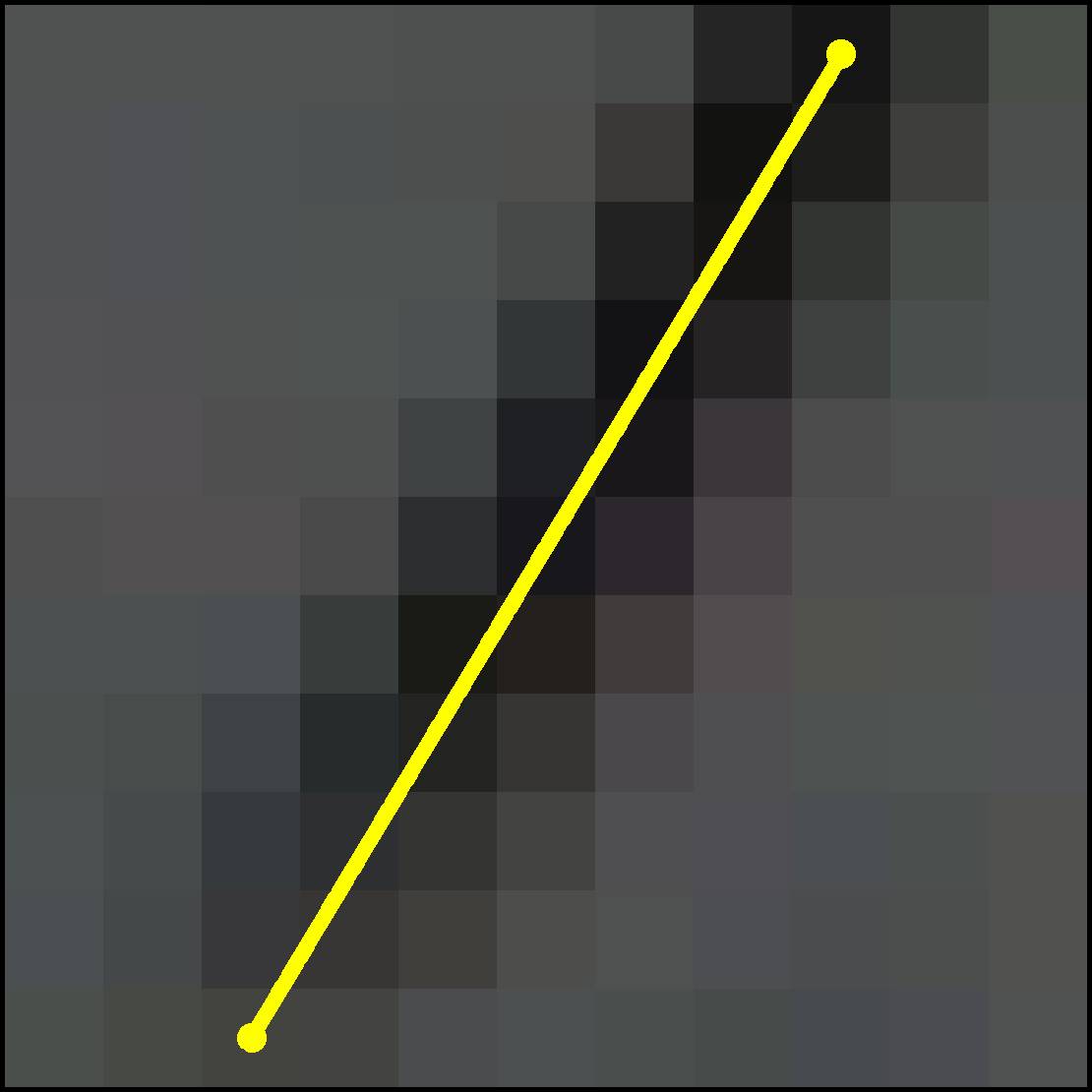
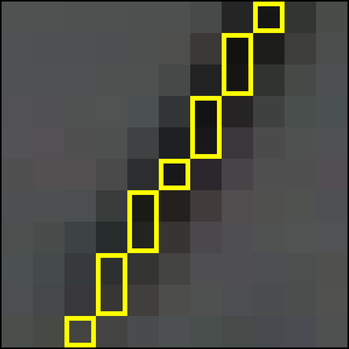
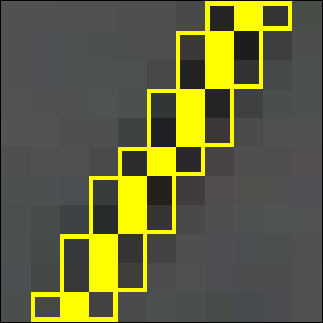
For additional robustness, we apply three smoothing procedures over the intensity profiles before computing the Fourier transform. First, a Gaussian blur is applied to the image. Then, the mean of parallel intensity profiles is computed, as illustrated by Figure 8. Finally, this mean is scaled to a length $l$ with linear interpolation. In our experiments, we have empirically chosen $l=30$.

(a)	(b)	(c)

Figure 8: Mean of intensity profiles. (a) The straight line between the two vertices of an arc. (b) The sequence of pixels intersected by the line. (c) The same pixels and one additional parallel sequence on each side: the Fourier transform is computed from a scaled mean of the three sequences.

7 Correspondence selection and pose estimation

The procedure for selecting or rejecting a keygraph correspondence in our implementation is a simple thresholding. For each vertex correspondence implied by the isomorphism, a dissimilarity function is applied to the descriptors, and the correspondence is rejected if one of the dissimilarities is higher than a certain threshold. The same verification is made for arcs, as illustrated by Figure 9.

(a) descriptors                  (b) dissimilarity                   (c) threshold

Figure 9: Example of keygraph correspondence selection using arc dissimilarity thresholding. (a) An isomorphism from a model keygraph with arc descriptors $\alpha_{m},\beta_{m},\gamma_{m}$ to a scene keygraph with arc descriptors $\alpha_{s},\beta_{s},\gamma_{s}$. (b) The three arc dissimilarities implied by the isomorphism. (c) The thresholding condition for selecting a correspondence.

Note that such procedure allows more than one correspondence per model graph or scene graph. The RANSAC-based pose estimation step is responsible for recognizing the correspondences that have been incorrectly selected and ignoring them. RANSAC is a probabilistic fitting procedure, specifically designed to handle high proportions of outliers. In general terms, it is based on iteratively choosing random sets of correspondences: for each set, a pose candidate is estimated and the number of correspondences that are inliers with respect to such candidate is stored as its score. The number of iterations is probabilistically adapted according to the best score: a high number of inliers implies a lower expected number of iterations before finding an optimal candidate. The actual number eventually reaches either this expected number or an upper bound, specified to avoid excessive running time. If the best score is sufficiently good when this happens, the respective candidate is chosen as the pose.

Given a set of keygraph correspondences $\Gamma$, a straightforward procedure for estimating the pose is applying RANSAC to the correspondences defined in equation (2) or over a set of frequent keypoint correspondences obtained with a voting table [55, 56, 24]. However, both procedures discard a valuable information: if a keygraph correspondence is correct, then all keypoint correspondences it implies are correct simultaneously. In our implementation, we apply RANSAC to a family of sets as equation (1). This reduces significatively the expected number of RANSAC iterations, as shown in Section 8.

8 Experimental results

Our implementation was written in C++ and based on the OpenCV library [8]. The Delaunay triangulation was computed with the Triangle library [48] and the Fourier transform was computed with the FFTW library [18]. In RANSAC, the best candidate is refined with the Levenberg-Marquardt algorithm [31, 35].

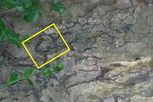
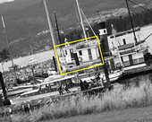
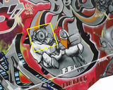
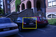
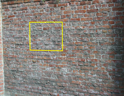
In our first experiment, we used image pairs manually obtained from the dataset shared by Mikolajczyk and Schmid [38]. This dataset is partitioned in $8$ subsets: each subset has one model, five scenes, and five homographies modelling the respective poses. The five scenes represent different degrees of a specific distortion. We chose $6$ subsets and, from each one, obtained the scene representing the lowest degree of distortion and a manually cropped sub-image of the model. Figure 10 shows the image pairs.

(a) bark	(b) bikes	(c) boat
(d) graf	(e) leuven	(f) wall

Figure 10: Image pairs used in the first experiment, with visual representations of the homographies. (a) bark: textured image with change of scale and rotation. (b) bikes: structured image with change of blur. (c) boat: structured image with change of scale and rotation. (d) graf: structured image with change of viewpoint. (e) leuven: structured image with change of brightness and contrast. (f) wall: textured image with change of viewpoint.

The objective of the experiment was comparing the accuracy of the three different structures shown in Section 5 for different images. We were interested in discovering the best structure for low-degree distortions before considering high-degree distortions. The $2$ subsets not chosen were trees, textured image with change of blur, and ubc, structured image with change of compression. Both were discarded for providing results excessively different: much worse for the former and much better for the latter.

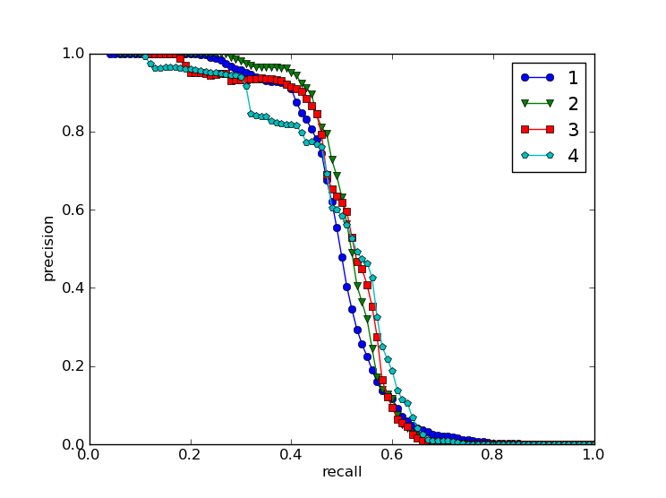
We cropped the models to bring the dataset closer to the case of object detection in cluttered backgrounds: the cropping significatively increases the number of scene images that have no correspondence in the model, raising the difficulty in particular for the textured images. The accuracy measure chosen was the recall-precision curve: recall is the fraction of correct correspondences that is selected, and precision is the fraction of selected correspondences that is correct. Those two values are computed for different thresholds and a curve is plotted accordingly.

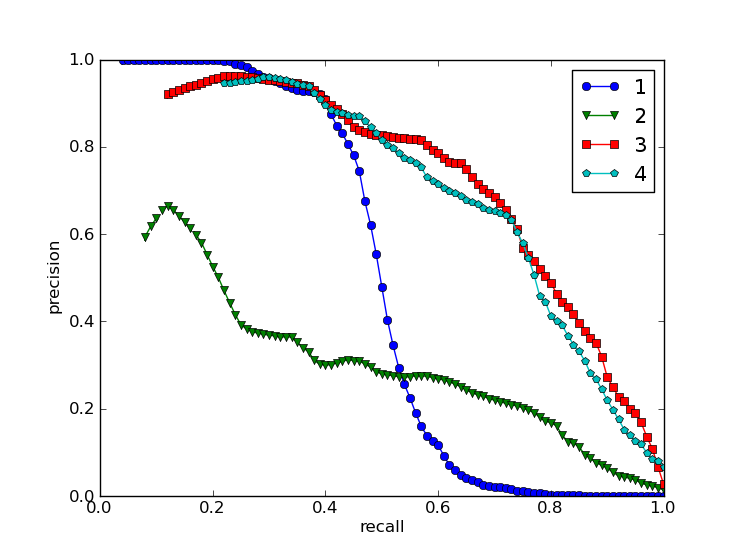
Since we were also interested in comparing the keygraph framework with the keypoint framework, we also plotted the precision-recall curve for individual keypoint correspondences. The keypoint descriptor chosen to select those correspondences was SIFT. In order to avoid bias for our method, we established that the recall is always computed from keypoint correspondences: in the case of keygraphs, such correspondences are obtained from equation (2).

Finally, we also established that a keygraph correspondence was correct if all its implied keypoint correspondences were correct, and a keypoint correspondence was correct if the Euclidean distance from the groundtruth was less than $3$ pixels. This value was chosen empirically. Figure 11 shows the results for two sequences of measurements: one with SIFT descriptors on vertices and one with Fourier descriptors on arcs. For both sequences the keypoint detector was the Hessian-Affine algorithm and the dissimilarity measure was the Euclidean distance.

(a) vertices with SIFT	(b) arcs with Fourier

Figure 11: Results for the two sequences of measurements in the first experiment: (a) for vertices with SIFT and (b) for arcs with Fourier. The name of each curve represents the number of vertices in the structure: the first one is the baseline curve for individual keypoint correspondences, hence the same in both sequences, and the other three are for the three structures shown in Section 5. Each curve is the mean of the curves across all pairs of images.

For vertices with SIFT, the similarity of all curves shows that naively using a state-of-the-art keypoint descriptor in the keygraph framework is not necessarily the best approach. For arcs with Fourier descriptors, we observed that keygraphs consistently had worse precisions for lower recalls, but consistently had better precisions for higher recalls. This was true even for the simplest structure with two vertices, which does not have the advantages of relative positioning, although its overall precision was much worse than the others. We also observed that the curves for the two circuits were similar. This discouraged us from trying larger circuits, as the difference in accuracy did not seem to justify the increase in running time.

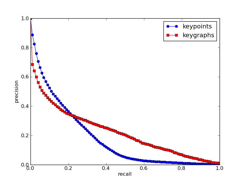
Because of its balance between accuracy and efficiency, circuits with three vertices were chosen to represent keygraphs in the second experiment. In this experiment, the objective was comparing exhaustively the keygraph framework with the keypoint framework. We kept the previous dataset and the idea of cropping, but used all $5$ degrees of all $8$ distortions and instead of cropping manually we randomly cropped $10$ models for each subset. Figure 12 shows the models and scenes for one of the subsets.

Figure 12: Models and scenes for the subset graf in the second experiment.

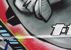
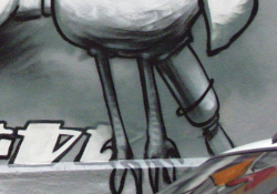
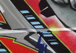
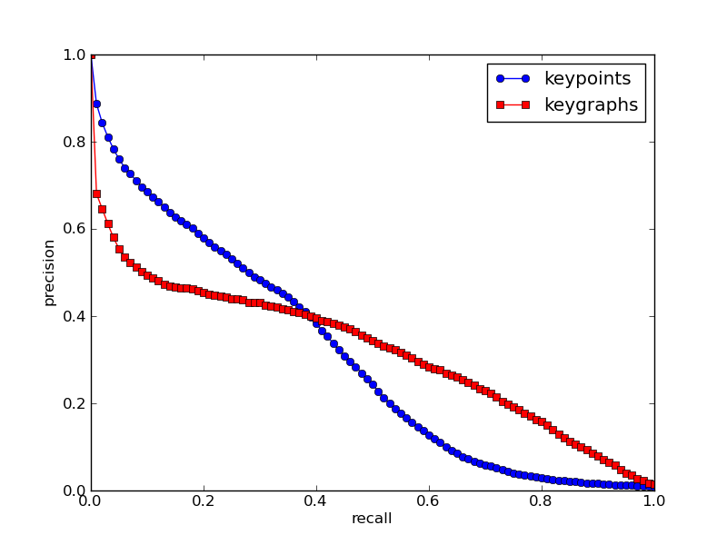
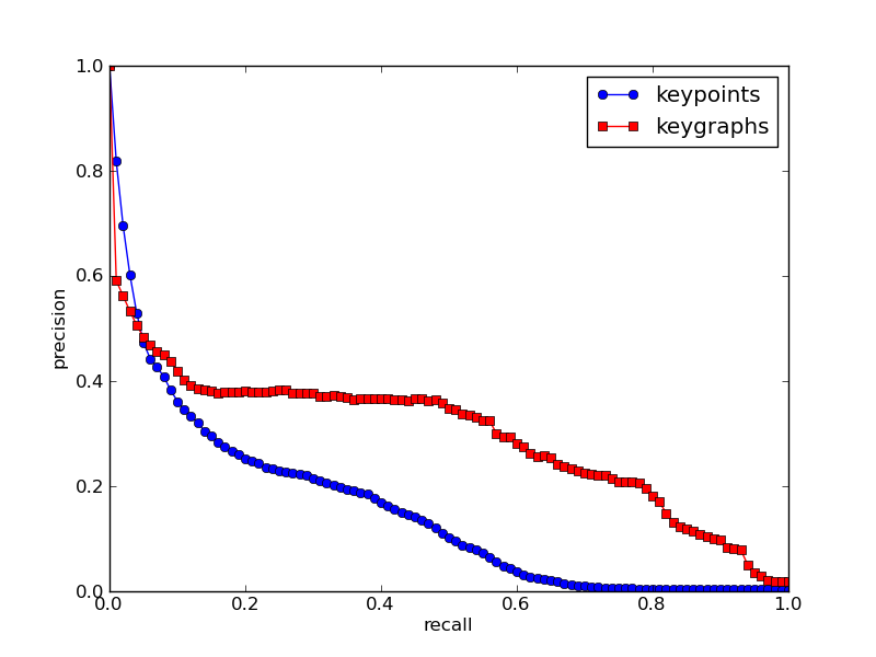
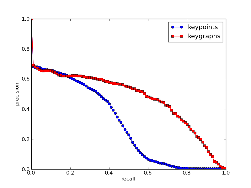
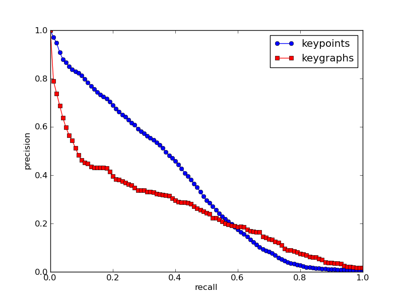
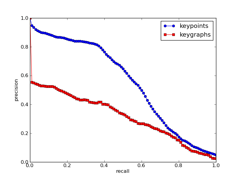
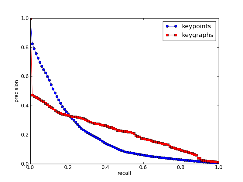
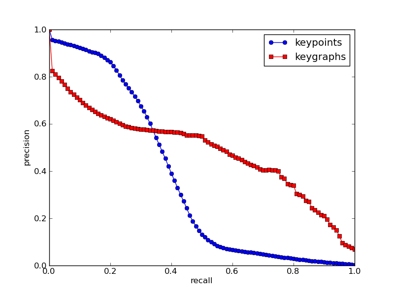
Furthermore, we made a sequence of measurements with the Hessian-Affine detector and a sequence of measurements with the MSER detector. In total, $800$ measurements were made and their results are shown in Figure 13. This second experiment confirmed that keygraphs provide superior precision for higher recalls. However, the specific recall where the curves intersect each other was not stable across subsets and detectors. Figure 14 shows that for two subsets keygraphs performed consistently better with Hessian-Affine. In contrast, Figure 15 shows that for two subsets keygraphs performed consistently worse with Hessian-Affine. With MSER the results for the same subsets were more similar to the average results, as illustrated by Figure 16.

(a) Hessian-Affine	(b) MSER

Figure 13: Results for the two sequences of measurements in the second experiment: (a) for Hessian-Affine and (b) for MSER. Each curve is the mean of the $200$ measurements taken for each keypoint detector.

(a) graf	(b) ubc

Figure 14: Results for the second experiment, specifically for Hessian-Affine and two subsets: (a) for graf and (b) for ubc. Each curve is the mean of $50$ measurements.

(a) bikes	(b) leuven

Figure 15: Results for the second experiment, specifically for Hessian-Affine and two subsets: (a) for bikes and (b) for leuven. Each curve is the mean of $50$ measurements.

(a) bikes	(b) leuven

Figure 16: Results for the second experiment, specifically for MSER and two subsets: (a) for bikes and (b) for leuven. Each curve is the mean of $50$ measurements.

These differences are particularly interesting because they are direct consequences of the advantages of each keypoint detector. In the comparative study of Mikolajczyk et al. [39], Hessian-Affine performed worse precisely on the bikes and leuven subsets. This shows that the keygraph framework is directly influenced by the repeatability of the keypoint detector chosen, but when good repeatability is ensured, then keygraphs present better precision at higher recalls.

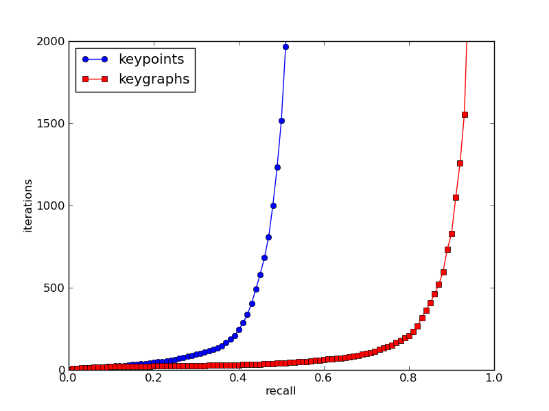
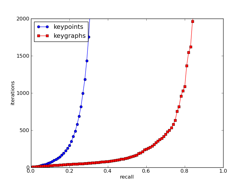
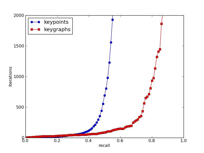
But that does not mean that detectors with worse repeatability should be necessarily dismissed. When using RANSAC, more important than the precision $p$ is the expected number of iterations, that can be approximated by

$$\frac{\log(1-\mathbb{P})}{\log(1-p^{h})}$$

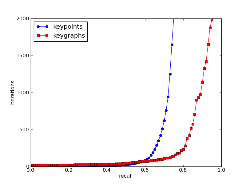
where $h$ is the size of the set of correspondences necessary for estimating a pose candidate. The value of $h$ is the fundamental difference between keypoints and keygraphs: for estimating an homography, four keypoint correspondences are needed. Therefore, $h=4$ for keypoints and $h=2$ for circuits with three vertices. The difference in number of iterations can be seen in Figure 17. As can be seen in Figure 18, even for the subsets where keygraphs had a consistently worse precision, they still had a consistently better number of iterations.

(a) Hessian-Affine	(b) MSER

Figure 17: Results for the two sequences of measurements in the second experiment: (a) for Hessian-Affine and (b) for MSER. Each curve is the mean of the $200$ measurements taken for each keypoint detector.

(a) bikes	(b) leuven

Figure 18: Results for the second experiment, specifically for Hessian-Affine and two subsets: (a) for bikes and (b) for leuven. Each curve is the mean of $50$ measurements.

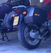
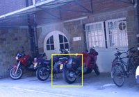
The objective of the third and final experiment was evaluating the running time of the keygraph framework and its viability for real-time applications. We wanted to verify if the implementation was capable of detecting an object on each frame given by a camera in reasonable time. Two sequences of tests were made: one with a fixed laptop webcam, whose screenshots are shown in Figure 19, and one with a PlayStation Eye camera, whose screenshots are shown in Figure 20.

Figure 19: Screenshots of object detection with a fixed laptop webcam.

Figure 20: Screenshots of object detection with a PlayStation Eye camera.

Both cameras were configured to give $640\times 480$ frames and all testes were made in a laptop with a Intel Core i5. Since the version of OpenCV used was not compiled with support to parallelism, the processing was made by a single 2.0 GHz core. For indexing the keygraphs, we indexed the Fourier arc descriptors using the FLANN library [43] and for each scene keytuple $(a_{s},b_{s},c_{S})$ we adopted the following procedure:

1	let $\mathcal{A}_{m}$ be the model arcs similar to $(a_{s},b_{s})$
2	let $\mathcal{B}_{m}$ be the model arcs similar to $(b_{s},c_{s})$
3	for each $(a_{m},b_{m})$ in $\mathcal{A}_{m}$
4	for each $(b^{\prime}_{m},c_{m})$ in $\mathcal{B}_{m}$ such that $b^{\prime}_{m}=b_{m}$
5	if $(c_{m},a_{m})$ and $(c_{s},a_{s})$ are similar
6	if $(a_{m},b_{m},c_{m})$ is the keytuple of a model keygraph
7	select the correspondence implied by $(a_{m},b_{m},c_{m})$ and $(a_{s},b_{s},c_{s})$

The threshold applied to the Euclidean distance of Fourier descriptors to decide whether two arcs were similar was $0.5$. For both tests, the average time for processing each frame was below $30$ms, which ensures at least $30$ frames per second. Using classic tracking techniques such as statistical filtering would certainly improve even further.

9 Conclusion

We have proposed a framework for object detection based on a generalization of keypoint correspondences into keygraph correspondences. The main difference of our approach to similar ones in the literature is that each step deals directly with graphs: the description does not need point region descriptors, the comparison takes the entire structure into consideration, and the pose estimation uses graph correspondences directly instead of converting them with a voting table. In order to show the viability of the framework, we also proposed an implementation with low theoretical complexity and performed experiments to prove both its accuracy and speed.

Besides testing different methods for keygraph detection and description, an interesting possibility for future research is developing keypoint detectors specifically tailored for building good keygraphs. A good step in this direction are the critical nets recently proposed by Gu et al. [19]. Another important step is showing that relatively powerful computers are not needed for applications based on the framework. Our implementation has been recently ported to a mobile phone, much more limited than the laptop used in the experiments of this paper, and had success in indoor sign detection [42].

References

- [1] M. Agrawal, K. Konolige, and M. R. Blas, CenSurE: Center Surround Extremas for realtime feature detection and matching, Proceedings of the 10th European Conference on Computer Vision: Part IV (D. Forsyth, P. Torr, and A Zisserman, eds.), Lecture Notes in Computer Science, vol. 5305, Springer, 2008, pp. 102–115.
- [2] D. H. Ballard, Generalizing the Hough transform to detect arbitrary shapes, Pattern Recognition 13 (1981), no. 2, 111–122.
- [3] S. Barton, V. Gouet-Brunet, M. Rukoz, C. Charbuillet, and G. Peeters, Estimating the indexability of multimedia descriptors for similarity searching, Proceedings of the 9th International Conference on Adaptivity, Personalization and Fusion of Heterogeneous Information, 2010, pp. 1–12.
- [4] , Qualitative comparison of audio and visual descriptors distributions, Proceedings of the 2010 International Conference on Multimedia Computing and Information Technology, 2010, pp. 101–104.
- [5] H. Bay, T. Tuytelaars, and L. van Gool, SURF: Speeded Up Robust Features, Computer Vision and Image Understanding 110 (2008), no. 3, 346–359.
- [6] S. Belongie, J. Malik, and J. Puzicha, Shape matching and object recognition using shape contexts, IEEE Transactions on Pattern Analysis and Machine Intelligence 24 (2002), no. 4, 509–522.
- [7] G. Bouchard and B. Triggs, Hierarchical part-based visual object categorization, Proceedings of the 2005 IEEE Computer Society Conference on Computer Vision and Pattern Recognition, vol. 1, IEEE Computer Society Press, 2005, pp. 710–715.
- [8] G. Bradski and A. Kaehler, Learning OpenCV: Computer vision with the OpenCV library, O’Reilly Media, 2008.
- [9] J. E. Bresenham, Algorithm for computer control of a digital plotter, IBM Systems Journal 4 (1965), no. 1, 25–30.
- [10] T. S. Caetano, L. Cheng, Q. V. Le, and A. J. Smola, Learning graph matching, Proceedings of the 11th IEEE International Conference on Computer Vision, IEEE Computer Society Press, 2007, pp. 1–8.
- [11] G. Carneiro and D. Lowe, Sparse flexible models of local features, Proceedings of the 9th European Conference on Computer Vision: Part III (A. Leonardis, H. Bischof, and A. Pinz, eds.), Lecture Notes in Computer Science, vol. 3953, Springer, 2006, pp. 29–43.
- [12] R. M. Cesar Jr., E. Bengoetxea, I. Bloch, and P. Larranaga, Inexact graph matching for model-based recognition: evaluation and comparison of optimization algorithms, Pattern Recognition 38 (2005), no. 11, 2099–2113.
- [13] D. Crandall, P. Felzenszwalb, and D. Huttenlocher, Spatial priors for part-based recognition using statistical models, Proceedings of the 2005 IEEE Computer Society Conference on Computer Vision and Pattern Recognition, vol. 1, IEEE Computer Society Press, 2005, pp. 10–17.
- [14] M. de Berg, O. Cheong, M. van Krefeld, and M. Overmars, Computational geometry: Algorithms and applications, third edition, Springer, 2008.
- [15] M. Ebrahimi and W. W. Mayol-Cuevas, SUSurE: Speeded Up Surround Extrema feature detector and descriptor for realtime applications, Proceedings of the 2009 IEEE Computer Society Conference on Computer Vision and Pattern Recognition, IEEE Computer Society Press, 2009, pp. 9–14.
- [16] M. A. Fischler and R. C. Bolles, Random Sample Consensus: a paradigm for model fitting with applications to image analysis and automated cartography, Communications of the ACM 24 (1981), no. 6, 381–395.
- [17] S. Fortune, A sweepline algorithm for Voronoi diagrams, Proceedings of the 2nd Annual Symposium on Computational Geometry, ACM Press, 1986, pp. 313–322.
- [18] M. Frigo and S. G. Johnson, The design and implementation of FFTW3, Proceedings of the IEEE 93 (2005), no. 2, 216–231.
- [19] S. Gu, Y. Zheng, and C. Tomasi, Critical nets and beta-stable features for image matching, Proceedings of the 11th European Conference on Computer Vision: Part III (K. Daniilidis, P. Maragos, and N. Paragios, eds.), Lecture Notes in Computer Science, vol. 6313, Springer, 2010, pp. 663–676.
- [20] C. G. Harris and M. J. Stephens, A combined corner and edge detector, Proceedings of the 4th Alvey Vision Conference, University of Sheffield Printing Unit, 1988, pp. 147–152.
- [21] M. Hashimoto and R. M. Cesar Jr., Object detection by keygraph classification, Proceedings of the 7th IAPR-TC-15 International Workshop on Graph-Based Representations in Pattern Recognition (A. Torsello, F. Escolano, and L. Brun, eds.), Lecture Notes in Computer Science, vol. 5534, Springer, 2009, pp. 223–232.
- [22] S. Hinterstoisser, S. Benhimane, and N. Navab, N3M: Natural 3D Markers for real-time object detection and pose estimation, Proceedings of the 11th IEEE International Conference on Computer Vision, IEEE Computer Society Press, 2007, pp. 1–7.
- [23] N. V. Hoang, V. Gouet-Brunet, M. Rukoz, and M. Manouvrier, Embedding spatial information into image content description for scene retrieval (in press), Pattern Recognition 43 (2010), no. 9, 3013–3024.
- [24] Y. Kanazawa and K. Uemura, Wide baseline matching using triplet vector descriptor, Proceedings of the 17th British Machine Vision Conference, vol. I, British Machine Vision Association, 2006, pp. 267–276.
- [25] A. Kandel, H. Bunke, and M. Last, Applied graph theory in computer vision and pattern recognition, Studies in Computational Intelligence, vol. 52, Springer, 2007.
- [26] Y. Ke and R. Sukthankar, PCA-SIFT: a more distinctive representation for local image descriptors, Proceedings of the 2004 IEEE Computer Society Conference on Computer Vision and Pattern Recognition, vol. 2, IEEE Computer Society Press, 2004, pp. 506–513.
- [27] W. G. Kropatsch, Benchmarking graph matching algorithms: a complementary view, Proceedings of the 3rd IAPR-TC-15 International Workshop on Graph-Based Representations in Pattern Recognition (J.-M. Jolion, W. G. Kropatsch, and M. Vento, eds.), CUEN, 2001, pp. 210–216.
- [28] S. Lazebnik, C. Schmid, and J. Ponce, Beyond bags of features: spatial pyramid matching for recognizing natural scene categories, Proceedings of the 2006 IEEE Computer Society Conference on Computer Vision and Pattern Recognition, vol. 2, IEEE Computer Society Press, 2006, pp. 2169–2178.
- [29] M. Leordeanu, M. Hebert, and R. Sukthankar, Beyond local appearance: category recognition from pairwise interactions of simple features, Proceedings of the 2007 IEEE Computer Society Conference on Computer Vision and Pattern Recognition, IEEE Computer Society Press, 2007, pp. 1–8.
- [30] V. Lepetit and P. Fua, Keypoint recognition using randomized trees, IEEE Transactions on Pattern Analysis and Machine Intelligence 28 (2006), no. 9, 1465–1479.
- [31] K. Levenberg, A method for the solution of certain non-linear problems in least squares, Quarterly of Applied Mathematics 2 (1944), no. 2, 164–168.
- [32] D. Lowe, Object recognition from local scale-invariant features, Proceedings of the 7th IEEE International Conference on Computer Vision, vol. 2, IEEE Computer Society Press, 1999, pp. 1150–1157.
- [33] , Distinctive image features from scale-invariant keypoints, International Journal of Computer Vision 20 (2004), no. 2, 91–110.
- [34] B. D. Lucas and T. Kanade, An iterative image registration technique with an application to stereo vision, Proceedings of the 7th International Joint Conference on Artificial Intelligence (P. J. Hayes, ed.), William Kaufmann, 1981, pp. 674–679.
- [35] D. Marquardt, An algorithm for least-squares estimation of nonlinear parameters, SIAM Journal on Applied Mathematics 11 (1963), no. 2, 431–441.
- [36] J. Matas, O. Chum, M. Urban, and T. Pajdla, Robust wide baseline stereo from maximally stable extremal regions, Proceedings of the 13th British Machine Vision Conference (D. Marshall and P. L. Rosin, eds.), British Machine Vision Association, 2002, pp. 384–396.
- [37] K. Mikolajczyk and C. Schmid, Scale & affine invariant interest point detectors, International Journal of Computer Vision 60 (2004), no. 1, 63–86.
- [38] , A performance evaluation of local descriptors, IEEE Transactions on Pattern Analysis and Machine Intelligence 27 (2005), no. 10, 1615–1630.
- [39] K. Mikolajczyk, T. Tuytelaars, C. Schmid, A. Zisserman, J. Matas, F. Schaffalitzky, T. Kadir, and L. van Gool, A comparison of affine region detectors, International Journal of Computer Vision 65 (2005), no. 1–2, 43–72.
- [40] H. Moravec, Obstacle avoidance and navigation in the real world by a seeing robot rover, Tech. report, Robotics Institute, Carnegie-Mellon University, 1980.
- [41] J. Morel and G. Yu, ASIFT: a new framework for fully affine invariant image comparison, SIAM Journal on Imaging Sciences 2 (2009), no. 2, 438–469.
- [42] H. Morimitsu, M. Hashimoto, R. B. Pimentel, R. M. Cesar Jr., and R. Hirata Jr., Keygraphs for sign detection in indoor environments by mobile phones, Proceedings of the 8th IAPR-TC-15 International Workshop on Graph-Based Representations in Pattern Recognition (X. Jiang, M. Ferrer, and A. Torsello, eds.), Lecture Notes in Computer Science, vol. 6658, Springer, 2011, pp. 315–324.
- [43] M. Muja and D. G. Lowe, Fast approximate nearest neighbors with automatic algorithm configuration, Proceedings of the 4th International Conference on Computer Vision Theory and Applications (A. Ranchordas and H. Araújo, eds.), vol. 1, INSTICC Press, 2009, pp. 331–340.
- [44] J. Philbin, O. Chum, M. Isard, J. Sivic, and A. Zisserman, Object retrieval with large vocabularies and fast spatial matching, Proceedings of the 2007 IEEE Computer Society Conference on Computer Vision and Pattern Recognition, IEEE Computer Society Press, 2007, pp. 1–8.
- [45] P. Punitha and D. S. Guru, Symbolic image indexing and retrieval by spatial similarity: an approach based on B-tree, Pattern Recognition 41 (2008), no. 6, 2068–2085.
- [46] E. Rosten and T. Drummond, Machine learning for high-speed corner detection, Proceedings of the 9th European Conference on Computer Vision: Part I (A. Leonardis, H. Bischof, and A. Pinz, eds.), Lecture Notes in Computer Science, vol. 3951, Springer, 2006, pp. 430–443.
- [47] C. Schmid and R. Mohr, Local grayvalue invariants for image retrieval, IEEE Transactions on Pattern Analysis and Machine Intelligence 19 (1997), no. 5, 530–535.
- [48] J. R. Shewchuk, Triangle: engineering a 2D quality mesh generator and Delaunay triangulator, Applied Computational Geometry: Towards Geometric Engineering (M¿ C. Lin and D. Manocha, eds.), Lecture Notes in Computer Science, vol. 1148, Springer, 1996, pp. 203–222.
- [49] J. Shi and C. Tomasi, Good features to track, Proceedings of the 1994 IEEE Computer Society Conference on Computer Vision and Pattern Recognition, IEEE Computer Society Press, 1994, pp. 593–600.
- [50] C. Silpa-Anan and R. Hartley, Optimised KD-trees for fast image descriptor matching, Proceedings of the 2008 IEEE Computer Society Conference on Computer Vision and Pattern Recognition, IEEE Computer Society Press, 2008, pp. 1–8.
- [51] B. Sirmacek and C. Unsalan, Urban area and building detection using SIFT keypoints and graph theory, IEEE Transactions on Geoscience and Remote Sensing 47 (2009), no. 4, 1156–1167.
- [52] J. Sivic, B. C. Russell, A. A. Efros, A. Zisserman, and W. T. Freeman, Discovering objects and their location in images, Proceedings of the 10th IEEE International Conference on Computer Vision, vol. 2, IEEE Computer Society Press, 2005, pp. 370–377.
- [53] J. Sivic and A. Zisserman, Video Google: efficient visual search of videos, Toward Category-Level Object Recognition (J. Ponce, M. Hebert, C. Schmid, and A. Zisserman, eds.), Lecture Notes in Computer Science, vol. 4170, Springer, 2006, pp. 127–144.
- [54] F. Tang and H. Tao, Object tracking with dynamic feature graph, Proceedings of the 2nd Joint IEEE International Workshop on Visual Surveillance and Performance Evaluation of Tracking and Surveillance, IEEE Computer Society Press, 2005, pp. 25–32.
- [55] D. Tell and S. Carlsson, Wide baseline point matching using affine invariants computed from intensity profiles, Proceedings of the 6th European Conference on Computer Vision: Part I (A. Heyden, G. Sparr, M. Nielsen, and P. Johansen, eds.), Lecture Notes in Computer Science, vol. 1842, Springer, 2000, pp. 814–828.
- [56] , Combining appearance and topology for wide baseline matching, Proceedings of the 7th European Conference on Computer Vision: Part I (D. Vernon, ed.), Lecture Notes in Computer Science, vol. 2350, Springer, 2002, pp. 68–81.
- [57] E. Tola, V. Lepetit, and P. Fua, DAISY: an efficient dense descriptor applied to wide baseline stereo, IEEE Transactions on Pattern Analysis and Machine Intelligence 32 (2010), no. 5, 815–830.
- [58] C. Tomasi and T. Kanade, Detection and tracking of point features, Tech. report, School of Computer Science, Carnegie-Mellon University, 1991.
- [59] T. Tuytelaars and K. Mikolajczyk, Local invariant feature detectors: a survey, Foundations and Trends in Computer Graphics and Vision 3 (2008), no. 3, 177–280.
- [60] M. Weber, M. Welling, and P. Perona, Unsupervised learning of models for recognition, Proceedings of the 6th European Conference on Computer Vision: Part I (D. Vernon, ed.), Lecture Notes in Computer Science, vol. 1842, Springer, 2000, pp. 18–32.
- [61] J. Yuan, Y. Wu, and M. Yang, Discovery of collocation patterns: from visual words to visual phrases, Proceedings of the 2007 IEEE Computer Society Conference on Computer Vision and Pattern Recognition, IEEE Computer Society Press, 2007, pp. 1–8.