The Elliptic Model for communication fluxes

Abstract

In this paper, a model (called Elliptic Model) is proposed to estimate the number of social ties between two locations using population data in a similar manner transportation research does with trips. To overcome the asymmetry of transportation models, the new model considers that the number of relationships between two locations is reversely proportional to the population in the ellipse whose focuses are in these two locations. The Elliptic Model is evaluated by considering the anonymous communications patterns of 25 million users from 3 different countries, where a location has been assigned to each user based on her most used phone tower or billing zip code. With this information, spatial social networks are built at three levels of resolution: tower, city and region for each of the three countries. The Elliptic Model reaches similar performance when predicting communication fluxes as transportation models do when predicting trips. This shows that human relationships are at least as influenced by geography as human mobility is.

1 Introduction

While social networks have been known for years to play a key role in various human phenomena [1, 2], during decades their study was limited to certain kind of social relationships for which interaction records were available, such as authorship and cooperation in science [3, 4]. Only recently it has been possible to map large social networks representing a broader range of interactions in order to explore how their structures influence processes occurring in these networks. The required large social network data sets, usually coming from telecommunication records originated in e-mail [5], phone [6] or online communication platforms [7], have been used to explore a wide range of topics such as adoption of innovation [8], social groups discovery [9, 10, 11], epidemic spreading [12, 13, 14], social mobilization [15] or sentiment spreading [16].

Despite the publication of such studies, network data is not widely available to the community due to legal, privacy or commercial issues. In addition, even with access to the electronic records, extracting a meaningful social network may be difficult at a large scale [6]. For these reasons, creating models that are able to mimic different social network properties have recently attracted a fair amount of research interest [17, 18, 19, 20, 21]. While most models try to generate synthetic networks with some desired characteristics (degree distribution and clustering coefficient among others), we will focus here on reproducing a macroscopic feature of real social networks: the number of social ties between different locations, i.e. how many relationships exist between two cities, two regions or even two neighborhoods. Throughout the paper, we will employ the term location to generically denote any of these three spatial aggregation levels. The creation of social connectivity maps between locations from widely accessible data, such as population geographic distribution (which is universally accessible for almost any region of the world through tools like Landscan), will prove useful for the study of information [22] or behaviour spreading in social networks among others [23].

The effect of geography on social networks

During the end of the 19th century and the beginnings of the 20th, a considerable amount of effort was dedicated to the development of telecommunication systems. Such systems, whether they carried written messages (telegraph) or voice (telephone), were designed to achieve a single goal: allowing people to communicate with those who are far away (indeed the Greek prefix tele- means distant). Interestingly (and contrary to some predictions from the beginning of the internet era [4] ) recent analyses of records from such system show that people do not commonly use them to talk to those far away, but with people who are actually close by. Precisely, it has been consistently found across records from emails, phones and blogs that the probability of a communication to ocurr between two people who are $r$ kilometres apart from each other follows a decay function, typically a power law [24, 25, 26, 27].

Although the communication fluxes between regions have not been the focus of much research yet, the above mentioned new evidences show that communication fluxes behave similar to trip fluxes and other phenomena driven by the distribution of population across the geographical space. In transportation research, flux prediction is a well-defined problem: given a set of locations $\{i,j,...\}$ whose coordinates and populations $\{n_{i},n_{j},...\}$ are known, the goal is inferring the flux matrix $T$ where each element $T_{ij}$ represents the number of trips from location $i$ to location $j$. The problem was traditionally approached using gravity models [28, 29, 30] which try to gather the effect of decaying probability with distance $r_{i,j}$ following the equation

$$T_{ij}\propto\frac{n_{i}^{\alpha}n_{j}^{\beta}}{f(r_{ij})}$$

where $\alpha$ and $\beta$ are fitting parameters usually estimated from training data, and $f(r_{ij})$ increases with distance, typically following an exponential or power-law function. A powerful idea was brought recently by the radiation model [31], which claims that it is not the distance that matters, but the amount of opportunities between $i$ and $j$, which can be estimated by the population in the area. In short, the authors explain that someone from rural Iowa is more likely to travel further to satisfy her needs than someone in New York City, given the latter has a handful of options within a few blocks. While in its original publication the radiation model included testing against a phone call dataset (see Figure 3 in [31]), the problem of predicting communication fluxes was not the main focus of any model to date. In this paper we will present a new model inspired by this radiation model which is able to predict communication fluxes surprisingly well. Actually, the accuracy is similar to the one reached by current transportation models when predicting trips.

2 Model description

Figure 1: Model scenario: $n_{i}$ represents the population of location $i$ while $s_{i\rightarrow j}$ represents the population within the circle with center in $i$ and radius up to $j$. As long as population is not homogeneously distributed $s_{i\rightarrow j}\neq s_{j\rightarrow i}$, the radiation model predictions will not be symmetrical. $e_{ij}$ represents the population within the smallest ellipse whose focuses are in $i$ and $j$ and contains both previous circles, as well as $n_{i}$ and $n_{j}$.

Formally, the radiation model, when applied to social relationships, estimates the communication flux $T_{ij}$ between two locations $i$ and $j$ using the population in both locations, and the population within the circle whose center is $i$ and radius equal to the distance between $i$ and $j$. Its formulation is

$$T_{i,j}^{rad}=K_{i}\frac{n_{i}n_{j}}{(n_{i}+s_{i\rightarrow j})(n_{i}+n_{j}+s_{i\rightarrow j})}$$

where $n_{i}$ represents the population of location $i$, $s_{i\rightarrow j}$ the number of people who are not in $i$ but closer to $i$ than $j$ and the normalization $K_{i}=n_{i}\frac{N_{T}}{N}$, where $N_{T}$ is the total number of relationships to predict (which in general is considered to be available) and $N=\sum_{i}n_{i}$ the total population.

It is straightforward to verify that $T^{rad}$ matrices are not symmetric in general. While asymmetry is a desirable feature for mobility models (commuting origin-destination matrices have strongly asymmetric suburbs-downtown fluxes) it is not when dealing with communication fluxes, because the number of relationships people from location $i$ have with people from location $j$ must be the same as the number of relationships people from $j$ have with people from $i$.

A natural modification of the radiation model to deal with communication fluxes could be a simple symmetrization of the model, which we will denote radBI and whose formulation is

$$T_{ij}^{radBI}=\frac{1}{2}(T_{ij}^{rad}+T_{ji}^{rad}).$$

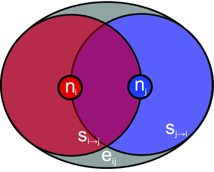
As shown below this model has a limited performance. This fact motivated us to develop the new model presented in this paper. Our model, which we will refer as the elliptic model (EM), is oriented to deal with social relationships. The EM considers that the probability of someone living at location i having an acquaintance at location $j$ is reversely proportional to the population of the area where both could meet provided their combined travel distance does not exceed certain threshold. This area forms an ellipse whose focuses are in locations $i$ and $j$. Among all possible ellipses the model selects the smallest one containing the two $r_{ij}$ radius circles whose centers are in $i$ and $j$ respectively (see Figure 1 for graphic explanation and comparison to the radiation model). Thus, the EM formulation is

$$T_{ij}^{ellip}=K\frac{n_{i}n_{j}}{e_{ij}}$$

where $e_{ij}$ is the population within the ellipse depicted in Figure 1 (note that $e_{ij}$ includes $n_{i}$ and $n_{j}$) and $K$ is a normalization parameter obtained from the total number of relationships to predict $N_{T}$ ( $\sum\limits_{i}\sum\limits_{j}T_{ij}^{ellip}=N_{T}$). Since $e_{ij}=e_{ji}$, $T_{ij}^{ellip}=T_{ji}^{ellip}$ and thus our model produces symmetrical matrices $T$.

In order to compare the quantities involved in the model, one needs to consider the sets $S_{i\rightarrow j}$ and $S_{j\rightarrow i}$ such as $\#S_{i\rightarrow j}=s_{i\rightarrow j}$ and $\#S_{j\rightarrow i}=s_{j\rightarrow i}$. Lets address the case of a very large city $C\subset S_{i\rightarrow j}$ whose population $n_{C}\approx e_{ij}$. While the radiation model predicts different fluxes depending on whether $C\subset(S_{i\rightarrow j}\cap S_{j\rightarrow i})$ or not (smaller when $C$ belongs to the intersection) the EM will provide the same prediction for both cases. In fact, since $e_{ij}\geq\#(S_{i\rightarrow j}\cup S_{j\rightarrow i})+n_{i}+n_{j}$ (and usually $e_{ij}\approx\#(S_{i\rightarrow j}\cup S_{j\rightarrow i})+n_{i}+n_{j}$) the role of the union set is the main contribution of the model.

3 Data description

To evaluate the performance of the EM, we compare it with a mobile phone data set containing Call Detail Records (CDRs) of a six month period in 3 different countries: France, Portugal, and Spain. In total, over 7 billion calls are considered to build the social graph for each country, whose links are included only if there is at least one call in both directions during the observation period. The result is an undirected graph (this is a common technique in the literature to avoid both marketing callers and misdialed calls [6]). In Table 1, some characteristics of the networks are presented, such as high clustering and relatively low average degree, which are expected from previous literature about mobile phone networks.

Country	Users $U$	Links $E$	$\langle k\rangle$	$\langle c\rangle$	$\frac{N}{Total\,Population}(\%)$
France	$18.7\cdot 10^{6}$	$81.3\cdot 10^{6}$	$8.73$	$0.16$	$30.21$
Portugal	$1.21\cdot 10^{6}$	$4.00\cdot 10^{6}$	$6.57$	$0.26$	$11.21$
Spain	$5.92\cdot 10^{6}$	$16.1\cdot 10^{6}$	$5.44$	$0.21$	$13.45$

Table 1: Characteristic properties of the social networks in the studied countries: number of users (Nodes) and relationships (Links), average degree $\langle k\rangle$, average clustering coefficient $\langle c\rangle$ and relative sample size of the users in the data set.

In addition to the communication records, our data include a location for each user: the most used mobile phone tower in France and Portugal and the billing zip code in Spain. In order to benchmark the multi-scale performance of the EM, three aggregation levels have been used: country-wide fluxes between cities and regions and on the other hand metropolitan fluxes within cities. Table 2 presents the number of locations considered in each aggregation level. When applying these spatial aggregations, the center of mass of the population is used as the higher level location, instead of the centroid of the region polygon (defined by administrative boundaries), in order to avoid undesirable effects in the fairly common case of a big city located in a corner of a polygon.

Country	Towers/Zip codes	Cities	Regions
France	17475	3520	96
Portugal	2209	297	20
Spain	8928	5446	52

Table 2: Number of locations considered in different geographic aggregation levels for each country. At the finer level, mobile phone towers are available France and Portugal, and zip codes for Spain. Aggregation is based on administrative boundaries: cities are cántons in France, concelhos in Portugal and municipios in Spain while regions mean départements in France, and provincias in Portugal and Spain.

4 Communication fluxes in country scale

To validate the predictions of the EM at large scale, we consider connectivity matrices $T$ in two aggregation levels. At the region level, matrix $T$ has thousands of elements while at the city level there are tens of millions of fluxes to predict (see Table 2). Input data for the predictions only consists of the location’s coordinates and populations, and the total number of relationships to predict $N_{T}$. Like the radiation model, the EM keeps the advantage of being parameter-free, so no training data is needed.

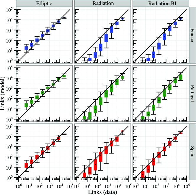
In Figure 2 we present a box-plot of the predictions from all the three models versus real data for fluxes between cities. The results prove consistently that the EM outperforms both the radiation model and its bilateral version. To present further evidence of the performance of the EM, we include in Table 3 the $R^{2}$ of the predictions in both aggregation levels. The results confirm that the EM outperforms previous models.

Overall, the accuracy of the predictions is similar to the one obtained when applying transportation models to trip prediction [31, 32]. This is an unexpected finding, since in principle, while there is an increasing cost (like time or energy) associated with distance when travelling, there is not such cost when making a phone call. While, as stated in the introduction, there were previous reports illustrating that social ties depend on physical distance, the capability of reproducing a significant portion of the distribution of social ties between locations just by employing a map placing them and their populations, highlights even more the importance of the geographical space when forming ties.

Figure 2: Predictions by different models versus real data. Fluxes between every city are presented, considering 297 cities in Portugal, 5446 in Spain, and 3520 in France. Error bars plot 10%, 30%, 50%, 70% and 90% quantiles. The elliptic model overcomes both radiation and bilateral radiation models in all three scenarios.

	France		Portugal		Spain
	City	Province	City	Province	City	Province
Radiation	0.534	0.615	0.621	0.776	0.556	0.588
RadiationBI	0.626	0.723	0.730	0.847	0.676	0.668
Elliptic	0.723	0.790	0.816	0.891	0.693	0.748

Table 3: $R^{2}$ of the different country-wide predictions. Note that these $R^{2}$ are calculated without any logarithmic transformation on data or predictions. The number of provinces considered is 97, 20 and 52, respectively. Since the number of cities is up to two orders of magnitude larger, the flux matrix $T$ is up to 4 orders of magnitude larger. While elliptic model is always more accurate than previous models, the improvement is specially remarkable in fluxes between cities.

5 Communication fluxes within cities

While previous literature already stated that distance influences the creation of social ties between cities, our dataset allows us to study also urban relationships by using the finer spatial aggregation level available: phone towers or zip codes. Predicting all possible tower to tower relationships within the country would imply dealing with a $T$ matrix with up to 300 million elements, with only less than 1% of them being not null. Thus, the prediction accuracy would be severely biased by the huge amount of zero cells. Instead, we study the short range accuracy of the model by applying it in each city where we got at least 20 different locations (the upper limit being Paris, where we have over 1000 mobile phone towers). In total, the analysis includes 40 cities in France, 29 Spain and 20 in Portugal.

Table 4 presents the results for the three algorithms in terms of average $R^{2}$. These results confirm that the EM still performs better, while the overall prediction accuracy is smaller compared to the country-wide experiment. The loss of accuracy within urban areas for any model purely based in distance is expected and observed in the transportation field [32]. One of the main reasons for this loss of accuracy is the fact that the distance is a poorer proxy for travel time or cost in cities. People in cities tend to be within a daily radius of action and the decision of whom they communicate with depends on other metrics related to the different hierarchies that could define a social distance (e.g. ethnicity, occupation, etc.) [25].

	France	Portugal	Spain
Radiation	0.377	0.527	0.434
RadiationBI	0.436	0.608	0.498
Elliptic	0.653	0.658	0.501

Table 4: Average $R^{2}$ for urban fluxes prediction for every city in the data set where there are at least 20 different locations (towers or zip codes). The number of locations range from this 20 up to 1000 in Paris. This sums up to 40 cities in France, 29 Spain and 20 in Portugal. Although the EM again outperforms previous models, each performance is small when compared to country-wide scenarios.

Correction $\varepsilon$ as a model improvement for urban areas

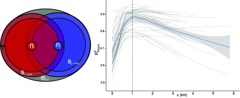
When applying the EM based on Figure 1 to urban relationships one should be aware that a tower $k$ whose distance to tower $i$ is $r_{ik}=r_{ij}+\varepsilon$ where $\varepsilon\ll r_{ij}$ will not be taken into account for predicting $T_{ij}$. Since towers tend to be closer to each other in urban areas, we propose the correction in Figure 3 for urban environments. The variation consists of including a correction parameter $\varepsilon$ so that the ellipse is now the smallest one containing the two circles of radius $r_{ij}+\varepsilon$ centered in $i$ and $j$. After studying several values of $\varepsilon$, we found that the prediction accuracy peaks near $\varepsilon=1$km for nearly all the cities (as shown in Figure 3).

There may be several interpretations for such a maximum: one could argue that it comes from the location error, known to be close to the average distance to neighbors from the Voronoi tessellation [33], which is around 1 km in average for our dataset. This agrees with the fact that the optimal $\varepsilon$ is a fixed value and does not depend on the distance $r$ between $i$ and $j$. On the other hand, when applied back to country-wide scenarios we found the correction term does not improve the predictions and no peak emerges near $\varepsilon\backsimeq r_{Voronoi}$ or elsewhere, reinforcing the hypothesis that within cities we are reaching the boundaries of the resolution of our location data.

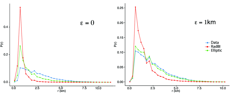
Another way to evaluate the performance of the different models is to compare them against empirical data in terms of the link-distance distribution $P(r)$ which represents the probability of observing a relationship between two people living $r$ kilometres from each other. Figure 4 shows the improvement $P(r)$ when applying the $\varepsilon=$1km correction. Without the correction term, short-range relationships are over represented, while the EM with the correction fits almost perfectly with the distribution obtained from the data. Note that although radiation model predictions also improve, it still predicts shorter relationships than those observed in the data.

Table 5 shows results of the corrected model for urban environments in terms of average $R^{2}$, which confirm a significant performance increase when applying the corrected model with $\varepsilon=1$ km across all cities in the data set.

Figure 3: Model modified for intracity predictions, adding the correction term $\varepsilon$. Each grey line represents a certain city in the dataset with the blue line and the shadow representing the general trend. We find predictions improve when some correction term is included, reaching a maximum around $\varepsilon=1\mbox{km}.$

Figure 4: Left: fraction of relationships $P(r)$ within distance $r$ in the real dataset compared to predictions by both elliptic and bilateral radiation models where $\varepsilon=0$ for Porto (Portugal). Right: elliptic prediction gets very close to data when using $\varepsilon=1\mbox{km}$. Although the radiation model predictions also improve, they still predict shorter relationships than those observed in reality.

	France	Portugal	Spain
Elliptic $\varepsilon=0$	0.670	0.645	0.494
Elliptic $\varepsilon=1\,\mbox{km}$	0.846	0.740	0.688

Table 5: Average $R^{2}$ of the predictions for the corrected model with $\varepsilon=1\mbox{km}$, compared to the original (non-corrected) model.

6 Conclusions and further research

In this paper the problem of predicting communication fluxes between different locations has been successfully addressed. A new model has been proposed to calculate the communication fluxes using only population distribution data. This data is publicly available worldwide through projects which provide population estimates for almost every square mile on earth.

The presented model successfully takes into account the symmetry of the communication fluxes, in order to predict the number of social ties between geographical locations at different scales, ranging from neighborhoods to regions. Interestingly, we have shown that geolocated population data is as useful to predict communication fluxes as it is to predict trip fluxes.

The proposed model is readily available to be used by researchers in different social sciences studying various phenomena where human ties are known to be crucial such as information propagation or disease spreading. Overall, our model implies social ties are to a large extent driven by geographical factors. While there may be other factors influencing very long distance relationships (e.g. time zones, or natural, national [34] and language borders [35], etc.) the available data did not allow to check them, so that further research would be needed along this line.

In order to enhance the employment of the EM by the research community, implementations in three widely used programming languages have been made available on our homepage [36], together with an interactive tool with France départments as an example scenario.

7 References

References

- [1] Mark S Granovetter. The strength of weak ties. American journal of sociology, pages 1360–1380, 1973.
- [2] Stanley Milgram. The small world problem. Psychology today, 2(1):60–67, 1967.
- [3] Benjamin F Jones, Stefan Wuchty, and Brian Uzzi. Multi-university research teams: shifting impact, geography, and stratification in science. Science, 322(5905):1259–1262, 2008.
- [4] Frances Cairncross. The death of distance: How the communications revolution will change our lives. Harvard Business Press, 2001.
- [5] Gueorgi Kossinets and Duncan J Watts. Empirical analysis of an evolving social network. Science, 311(5757):88–90, 2006.
- [6] J-P Onnela, Jari Saramäki, Jorkki Hyvönen, György Szabó, David Lazer, Kimmo Kaski, János Kertész, and A-L Barabási. Structure and tie strengths in mobile communication networks. Proceedings of the National Academy of Sciences, 104(18):7332–7336, 2007.
- [7] Alan Mislove, Massimiliano Marcon, Krishna P Gummadi, Peter Druschel, and Bobby Bhattacharjee. Measurement and analysis of online social networks. In Proceedings of the 7th ACM SIGCOMM conference on Internet measurement, pages 29–42. ACM, 2007.
- [8] Jameson L Toole, Meeyoung Cha, and Marta C González. Modeling the adoption of innovations in the presence of geographic and media influences. PloS one, 7(1):e29528, 2012.
- [9] Jaewon Yang and Jure Leskovec. Community-affiliation graph model for overlapping network community detection. In Data Mining (ICDM), 2012 IEEE 12th International Conference on, pages 1170–1175. IEEE, 2012.
- [10] Yong-Yeol Ahn, James P Bagrow, and Sune Lehmann. Link communities reveal multiscale complexity in networks. Nature, 466(7307):761–764, 2010.
- [11] Vincent D Blondel, Jean-Loup Guillaume, Renaud Lambiotte, and Etienne Lefebvre. Fast unfolding of communities in large networks. Journal of Statistical Mechanics: Theory and Experiment, 2008(10):P10008, 2008.
- [12] Romualdo Pastor-Satorras and Alessandro Vespignani. Epidemic spreading in scale-free networks. Physical review letters, 86(14):3200, 2001.
- [13] Pu Wang, Marta C González, Cesar A Hidalgo, and Albert-László Barabási. Understanding the spreading patterns of mobile phone viruses. Science, 324(5930):1071–1076, 2009.
- [14] Christian M Schneider, Tamara Mihaljev, Shlomo Havlin, and Hans J Herrmann. Suppressing epidemics with a limited amount of immunization units. Physical Review E, 84(6):061911, 2011.
- [15] Galen Pickard, Wei Pan, Iyad Rahwan, Manuel Cebrian, Riley Crane, Anmol Madan, and Alex Pentland. Time-critical social mobilization. Science, 334(6055):509–512, 2011.
- [16] James H Fowler and Nicholas A Christakis. Dynamic spread of happiness in a large social network: longitudinal analysis over 20 years in the framingham heart study. BMJ: British medical journal, 337, 2008.
- [17] Duncan J Watts and Steven H Strogatz. Collective dynamics of "small-world" networks. nature, 393(6684):440–442, 1998.
- [18] Albert-László Barabási and Réka Albert. Emergence of scaling in random networks. science, 286(5439):509–512, 1999.
- [19] Brian Karrer and MEJ Newman. Random graphs containing arbitrary distributions of subgraphs. Physical Review E, 82(6):066118, 2010.
- [20] Petter Holme and Beom Jun Kim. Growing scale-free networks with tunable clustering. Physical Review E, 65(2):026107, 2002.
- [21] Carlos Herrera and Pedro J Zufiria. Generating scale-free networks with adjustable clustering coefficient via random walks. In Network Science Workshop (NSW), 2011 IEEE, pages 167–172. IEEE, 2011.
- [22] Thomas J Allen. Managing the flow of technology: Technology transfer and the dissemination of technological information within the r&d organization. MIT Press Books, 1, 1984.
- [23] Juan Fernández-Gracia, Krzysztof Suchecki, José J Ramasco, Maxi San Miguel, and Víctor M Eguíluz. Is the voter model a model for voters? arXiv preprint arXiv:1309.1131, 2013.
- [24] Gautier Krings, Francesco Calabrese, Carlo Ratti, and Vincent D Blondel. Urban gravity: a model for inter-city telecommunication flows. Journal of Statistical Mechanics: Theory and Experiment, 2009(07):L07003, 2009.
- [25] Carlos Herrera-Yagüe, Christian M Schneider, Thomas Couronne, Zbigniew Somoreda, Rosa M Benito, Pedro J Zufiria, and Marta C González. Understanding social structures behind the six degrees of separation. under review, 2013.
- [26] David Liben-Nowell, Jasmine Novak, Ravi Kumar, Prabhakar Raghavan, and Andrew Tomkins. Geographic routing in social networks. Proceedings of the National Academy of Sciences of the United States of America, 102(33):11623–11628, 2005.
- [27] Santi Phithakkitnukoon, Zbigniew Smoreda, and Patrick Olivier. Socio-geography of human mobility: A study using longitudinal mobile phone data. PloS one, 7(6):e39253, 2012.
- [28] Sven Erlander and Neil F Stewart. The gravity model in transportation analysis: theory and extensions, volume 3. Vsp, 1990.
- [29] Rosalind M Eggo, Simon Cauchemez, and Neil M Ferguson. Spatial dynamics of the 1918 influenza pandemic in england, wales and the united states. Journal of The Royal Society Interface, 8(55):233–243, 2011.
- [30] Duygu Balcan, Vittoria Colizza, Bruno Gonçalves, Hao Hu, José J Ramasco, and Alessandro Vespignani. Multiscale mobility networks and the spatial spreading of infectious diseases. Proceedings of the National Academy of Sciences, 106(51):21484–21489, 2009.
- [31] Filippo Simini, Marta C González, Amos Maritan, and Albert-László Barabási. A universal model for mobility and migration patterns. Nature, 484(7392):96–100, 2012.
- [32] Yingxiang Yang, Carlos Herrera-Yagüe, Nathan Eagle, and Marta C González. A multi-scale study of commuting patterns incorporating digital traces. under review, 2013.
- [33] Michael Ulm and Peter Widhalm. Properties of the positioning error of cell phone trajectories. under review, 2013.
- [34] Johan Ugander, Brian Karrer, Lars Backstrom, and Cameron Marlow. The anatomy of the facebook social graph. arXiv preprint arXiv:1111.4503, 2011.
- [35] Vincent Blondel, Gautier Krings, and Isabelle Thomas. Regions and borders of mobile telephony in belgium and in the brussels metropolitan zone. Brussels Studies, 42(4), 2010.
- [36] http://humnetlab.mit.edu/elliptic. 2013.