Nonequilibrium transport through a quantum dot coupled to normal and superconducting leads

Abstract

We study the interacting quantum dot coupled to the normal and superconducting leads by means of a continuous-time quantum Monte Carlo method in the Keldysh-Nambu formalism. Deducing the steady current through the quantum dot under a finite voltage, we examine how the gap magnitude in the superconducting lead and the interaction strength at the quantum dot affect transport properties. It is clarified that the Andreev reflection and Kondo effect lead to nonmonotonic behavior in the nonequilibrium transport at zero temperature.

1 Introduction

Electron transport through nanofabrications has attracted interests. One of the interesting systems is the quantum dot system coupled to the normal and superconducting leads, which has experimentally been realized [1, 2, 3]. It has recently been examined how the Kondo effect due to electron correlations competes with the proximity-induced on-dot pairing effects [4]. Theoretical study for the system has been done by many groups  [5, 6, 9, 7, 8, 11, 10, 12] and some interesting transport properties have successfully been explained. However, it is not clear how the current are affected by the local correlations and Andreev reflection quantitatively. This may be crucial to understand the experimental results correctly since the linear response region, which can be treated quantitatively by means of the numerical renormalization group method, is narrow in the interacting quantum dot system. Therefore, another unbiased method is desired to discuss the nonlinear response in the system. One of the appropriate techniques is the continuous-time quantum Monte Carlo (CTQMC) method [13] based on the Keldysh formalism [14, 15]. In our previous paper [17], we have used the CTQMC method in the Nambu formalism to discuss the nonequilibrium transport properties in the quantum dot coupled to the normal and superconducting leads. However, the analysis was restricted in the simple case and it is still unclear how the superconducting gap affects transport properties for the quantum dot system.

To clarify this, we consider the interacting quantum dot coupled to the normal and superconducting leads. Calculating the time evolution of the current through the quantum dot at zero temperature, we examine how the gap magnitude in the superconducting lead affects the nonequilibrium transport. It is clarified that the Andreev reflection and Kondo effect lead to nonmonotonic behavior in the steady current.

This paper is organized as follows. In Sec. 2, we introduce the model Hamiltonian and briefly explain the CTQMC algorithm in the Keldysh-Nambu formalism. In Sec. 3, we discuss the nonequilibrium phenomena in the quantum-dot system. A summary is given in Sec. 4.

2 Model and Method

We consider the interacting quantum dot coupled to the normal and superconducting leads. For simplicity, we use a single level quantum dot with the Coulomb interaction $U$ and assume the superconducting lead to be described by the BCS theory with an isotropic gap $\Delta$. The model Hamiltonian should be given as

$$H = H_{0}+H^{\prime},$$ (1)

$$H_{0} = \sum_{k\alpha\sigma}\left(\epsilon_{k\alpha}-\mu_{\alpha}\right)c_{k\alpha\sigma}^{\dagger}c_{k\alpha\sigma}+\Delta\sum_{k}\left(c_{-kS\downarrow}^{\dagger}c_{kS\uparrow}^{\dagger}+c_{kS\uparrow}c_{-kS\downarrow}\right)$$ (2)

$$+ \sum_{k\alpha\sigma}\left(V_{k\alpha}c_{k\alpha\sigma}^{\dagger}d_{\sigma}+V_{k\alpha}^{*}d_{\sigma}^{\dagger}c_{k\alpha\sigma}\right)+\sum_{\sigma}\left(\epsilon_{d}+\frac{U}{2}\right)n_{\sigma},$$

$$H^{\prime} = U\left(n_{\uparrow}n_{\downarrow}-\frac{1}{2}\sum_{\sigma}n_{\sigma}\right),$$ (3)

where $c_{k\alpha\sigma}(c_{k\alpha\sigma}^{\dagger})$ is the annihilation (creation) operator of an electron with wave vector $k$ and spin $\sigma(=\uparrow,\downarrow)$ in the $\alpha$th lead. $d_{\sigma}(d_{\sigma}^{\dagger})$ is the annihilation (creation) operator of an electron at the quantum dot and $n_{\sigma}=d_{\sigma}^{\dagger}d_{\sigma}$. $\epsilon_{k\alpha}$ is the dispersion relation of the $\alpha$th lead, $V_{k\alpha}$ is the hybridization between the $\alpha$th lead and the quantum dot, and $\epsilon_{d}$ is the energy level. We set the chemical potential in each lead as $\mu_{N}=V$ and $\mu_{S}=0$, where $V$ is the bias voltage. We here consider the system with $\epsilon_{d}+U/2=0$ in the infinite bandwidth limit, where the coupling $\Gamma_{\alpha}(\omega)=\pi\sum_{k}\left|V_{k\alpha}\right|^{2}\delta(\omega-\epsilon_{k\alpha})$ is constant.

In this study, we use the weak-coupling version of the CTQMC method based on the Keldysh formalism [14, 15]. In the method, we simulate the system prepared in the noninteracting nonequilibrium state with the interaction turned on at time $t=0$. Therefore, the simulation may be referred to as an ”interaction quench”. When fluctuations due to the interaction quench relaxes and the system converges, we can discuss steady-state properties in the framework.

We first consider the following identity as

$$1 = {\rm Tr}\left[\rho_{0}e^{it\left(H_{0}+H^{\prime}-K/t\right)}e^{-it\left(H_{0}+H^{\prime}-K/t\right)}\right],$$ (4)

where $\rho_{0}=e^{-\beta H_{0}}/{\rm Tr}\Big{[}e^{-\beta H_{0}}\Big{]}$ and $K$ is a nonzero constant. By expanding two exponentials in eq. (4) in terms of the interaction representation, we obtain as

$$1 = {\rm Tr}\Big{\{}\rho_{0}\tilde{T}\left[\exp\Big{\{}i\int_{0}^{t}d\tilde{t}\left(H^{\prime}(\tilde{t})-\frac{K}{t}\right)\Big{\}}\right]e^{itH_{0}}$$

$$\times e^{-itH_{0}}T\left[\exp\Big{\{}-i\int_{0}^{t}dt\left(H^{\prime}(t)-\frac{K}{t}\right)\Big{\}}\right]\Big{\}},$$

$$= \sum_{l}\Big{(}-\frac{iK}{t}\Big{)}^{l}\int_{0}^{t}d\tilde{t}_{1}\cdots\int_{\tilde{t}_{l-1}}^{t}d\tilde{t}_{l}\sum_{m}\Big{(}\frac{iK}{t}\Big{)}^{m}\int_{0}^{t}dt_{1}\cdots\int_{t_{m-1}}^{t}dt_{m}$$

$$\times {\rm Tr}\Big{[}\rho_{0}e^{i\tilde{t}_{1}H_{0}}\Big{(}1-\frac{t}{K}H^{\prime}\Big{)}\cdots e^{i(\tilde{t}_{l}-\tilde{t}_{l-1})H_{0}}\Big{(}1-\frac{t}{K}H^{\prime}\Big{)}e^{i(t-\tilde{t}_{l})H_{0}}$$

$$\times e^{-i(t-t_{m})H_{0}}\Big{(}1-\frac{t}{K}H^{\prime}\Big{)}\cdots e^{-i(t_{2}-t_{1})H_{0}}\Big{(}1-\frac{t}{K}H^{\prime}\Big{)}e^{-it_{1}H_{0}}\Big{]},$$

where $T(\tilde{T})$ is the time-ordering (antitime-ordering) operator. By using the following equation as

$$1-\frac{t}{K}H^{\prime}=1-\frac{tU}{K}\left(n_{\uparrow}n_{\downarrow}-\frac{1}{2}\sum_{\sigma}n_{\sigma}\right)=\frac{1}{2}\sum_{s=\pm 1}e^{\gamma s(n_{\uparrow}-n_{\downarrow})},$$ (5)

with $\gamma=\cosh^{-1}(1+tU/2K)$, the identity is represented as

$$1 = \sum_{lm}(-i)^{l}i^{m}\left(\frac{K}{2t}\right)^{l+m}\sum_{\{\tilde{s}\}\{s\}}\int_{0}^{t}d\tilde{t}_{1}\cdots\int_{\tilde{t}_{l-1}}^{t}d\tilde{t}_{l}\int_{0}^{t}dt_{1}\cdots\int_{t_{m-1}}^{t}dt_{m}$$ (6)

$$\times \!\!\!\!{\rm Tr}\Big{[}\rho_{0}e^{i{\tilde{t}}_{1}H_{0}}e^{\gamma\tilde{s}_{1}(n_{\uparrow}-n_{\downarrow})}\cdots e^{\gamma\tilde{s}_{l}(n_{\uparrow}-n_{\downarrow})}e^{-i({\tilde{t}}_{l}-t_{m})H_{0}}e^{\gamma s_{m}(n_{\uparrow}-n_{\downarrow})}\cdots e^{\gamma s_{1}(n_{\uparrow}-n_{\downarrow})}e^{-it_{1}H_{0}}\Big{]}.$$

The introduction of the Ising valuable $s$ in eq. (5) allows us to perform Monte Carlo simulations. An $(l+m)$th order configuration $c=\{s_{k_{1}},s_{k_{2}},\cdots,s_{k_{n}};t_{k_{1}},t_{k_{2}},\cdots,t_{k_{n}}\}$ is represented by the auxiliary spins $s_{k_{1}},s_{k_{2}},\cdots,s_{k_{n}}$ at the Keldysh times $t_{k_{1}},t_{k_{2}},\cdots,t_{k_{n}}$ along the Keldysh contour, where the $l(m)$ denotes the number of spins on the forward (backward) contour and $n=l+m$ (see Fig. 1). Its weight $w_{c}$ is then given as

$$w_{c} = (-i)^{l}i^{m}\left(\frac{Kdt}{2t}\right)^{n}\det\left[{\hat{N}}^{(n)}\right]^{-1},$$ (7)

where ${\hat{N}}$ is an $n\times n$ matrix and its element consists of a $2\times 2$ matrix [16] as $\left[{\hat{N}}^{(n)}\right]^{-1}={\hat{\Gamma}}^{(n)}-{\hat{g}}^{(n)}\left({\hat{\Gamma}}^{(n)}-{\hat{I}}^{(n)}\right)$, ${\hat{I}}^{(n)}_{ij}=\delta_{ij}{\hat{\sigma}}_{0}$, ${\hat{\Gamma}}^{(n)}_{ij}=\delta_{ij}\exp\left({\gamma s_{k_{i}}{\hat{\sigma}}_{z}}\right)$, and ${\hat{g}}^{(n)}_{ij}={\hat{\sigma}}_{z}{\hat{G}}_{0}(t_{k_{i}},t_{k_{j}})$, where ${\hat{\sigma}}_{0}$ is the identity matrix and ${\hat{\sigma}}_{z}$ is the $z$-component of the Pauli matrix. The matrix ${\hat{G}}_{0}$ is given by the lesser and greater Green’s functions as

$${\hat{G}}_{0}(t^{\prime}_{k},t^{\prime\prime}_{k})=\left\{\begin{array}[]{cc}{\hat{G}}_{0}^{<}(t^{\prime},t^{\prime\prime})&t^{\prime}_{k}<t^{\prime\prime}_{k}\\ {\hat{G}}_{0}^{>}(t^{\prime},t^{\prime\prime})&t^{\prime}_{k}\geq t^{\prime\prime}_{k}\end{array}\right.,$$ (8)

where the times $t^{\prime}$ and $t^{\prime\prime}$ correspond to the Keldysh times $t_{k}^{\prime}$ and $t_{k}^{\prime\prime}$. These Green’s functions have been obtained by the standard technique [11, 8]. We note that the weight for a certain configuration is represented by the complex number. This should yield serious dynamical sign problem if simulations are performed on the longer contours. Therefore, accurate calculations are restricted to a certain time $t_{max}$.

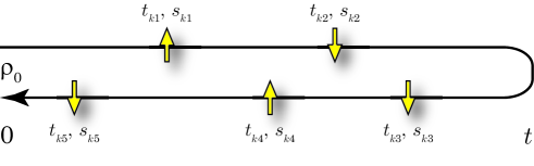
Figure 1: (Color online) Illustration of the Keldysh contour for the CTQMC method. Arrows represent auxiliary Ising spins for a certain configuration corresponding to the perturbation order $l=2$ and $m=3\;\;(n=5)$.

To perform Monte Carlo simulations, we use the Metropolis algorithm with the simple sampling process, where an Ising spin is inserted or removed in the Keldysh contour in each Monte Carlo step. Here, we measure the current from the quantum dot to $\alpha$th lead $I_{\alpha}$, which is defined as $I_{\alpha}=-2{\rm Im}\sum_{k\alpha}V_{k\alpha\sigma}\langle c_{k\alpha\sigma}^{\dagger}d_{\sigma}\rangle$. The detail of the measurement formula is given in Ref. [17]. In this study, we use the coupling constant of the normal lead $\Gamma_{N}$ as the unit of energy and fix the parameters as $\Gamma_{S}/\Gamma_{N}=1$, $V/\Gamma_{N}=0.5$, and $T/\Gamma_{N}=0$. In the following, we perform the CTQMC simulations to discuss the nonequilibrium transport in a quantum dot coupled to normal and superconducting leads.

3 Results

In the section, we discuss how the gap magnitude affects the steady current through the interacting quantum dot. By performing CTQMC simulations, we calculate the time evolution of the currents $I_{N}$ and $-I_{S}$ with a fixed voltage $V/\Gamma_{N}=0.5$, as shown in Fig. 2.

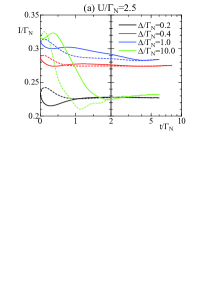
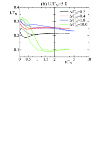
Figure 2: (Color online) Time evolution of the currents for the system with $V/\Gamma_{N}=0.5$ and $T/\Gamma_{N}=0$ when $U/\Gamma_{N}=2.5(a)$ and $5.0$ (b). Solid (dashed) lines represent the currents from the quantum dot to the normal (superconducting) lead.

In the figure, quantities are shown on the linear plot in the initial relaxation region ($t\Gamma_{N}<2$) and on the logarithmic plot in the rest ($t\Gamma_{N}>2$). When $t\Gamma_{N}=0$, the steady current $(I=I_{N}=-I_{S})$ flows through the noninteracting quantum dot. The introduction of the interaction yields oscillation behavior in both currents ($I_{N}$ and $-I_{S}$). Although two currents are different in the transient region, we find that each oscillation behavior is quickly damped and these currents approach a certain value when the time proceeds, as shown in Fig. 2. Therefore, in the case, the current at $t=t_{max}$ can be regarded as the steady current.

When $\Delta/\Gamma_{N}\lesssim 0.5$, there is not so large difference between the currents at $t\Gamma_{N}=0$ and $t=t_{max}$ although the oscillation behavior appears in the initial relaxation, as shown in Fig. 2 (a). This means that the interaction at the quantum dot little affects the steady current. In fact, the increase of the gap magnitude monotonically increases the steady current, which is similar to that for the noninteracting case. Therefore, we can say that when the gap magnitude is small enough, the Andreev reflection is dominant and the Kondo effect little affects transport properties.

On the other hand, when $\Delta/\Gamma_{N}\gtrsim 0.5$, the steady current is suppressed by the increase of the gap magnitude, as shown in Figs. 2 (a) and (b). This behavior may be explained by the following. The Coulomb interaction at the quantum dot induces the Kondo resonance peak around the chemical potential. On the other hand, the energy level for an electron with an opposite spin pairing with the electron is away from the chemical potential and its density of states decreases due to the Kondo effect. Therefore, the Andreev transport under the finite voltage is strongly suppressed. In a larger gap case, the Andreev current little flows and the system may be regarded as an insulating state.

By performing similar calculations, we obtain the density plot of the steady current, as shown in Fig. 3.

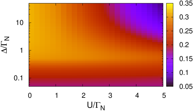
Figure 3: (Color online) Density plot of the normalized steady current $I/\Gamma_{N}$ through the quantum dot system with $V/\Gamma_{N}=0.5$ and $T/\Gamma_{N}=0$.

In the noninteracting case with $U/\Gamma_{N}=0$, the increase of the gap magnitude monotonically increases the steady current, which should be induced by the Andreev reflections. On the other hand, the introduction of the interaction leads to different behavior, where the development of the Kondo peak around the chemical potential suppresses the Andreev reflection. Therefore, in the larger $U$ and $\Delta$ region, the steady current is strongly suppressed.

4 Summary

We study nonequilibrium transport through the interacting quantum dot coupled to the normal and superconducting leads by means of a continuous-time quantum Monte Carlo method in the Keldysh-Nambu formalism. Calculating the time evolution of the current through the quantum dot, we discuss how the gap magnitude in the superconducting lead and the interaction at the quantum dot affect the steady current. We have found that nonmonotonic behavior is induced by the competition between the Kondo effect and the Andreev reflections.

References

- [1] M. R. Gräber, T. Nussbaumer, W. Belzig, and C. Schönenberger: Nanotechnology 15 (2004) S479.
- [2] L. Hofstetter, S. Csonka, J. Nygard, and C. Schönenberger: Nature (London) 461 (2009) 960.
- [3] L. G. Herrmann, F. Portier, P. Roche, A. L. Yeyati, T. Kontos, and C. Strunk: Phys. Rev. Lett. 104 (2010) 026801.
- [4] R. S. Deacon, Y. Tanaka, A. Oiwa, R. Sakano, K. Yoshida, K. Shibata, K. Hirakawa, and S. Tarucha: Phys. Rev. Lett. 104 (2010) 076805; Phys. Rev. B 81 (2010) 121308.
- [5] R. Fazio and R. Raimondi: Phys. Rev. Lett. 80 (1998) 2913.
- [6] P. Schwab and R. Raimondi: Phys. Rev. B 59 (1999) 1637.
- [7] A. A. Clerk, V. Ambegaokar, and S. Hershfield: Phys. Rev. B 61 (2000) 3555.
- [8] J. C. Cuevas, A. Levy Yeyati, and A. Martin-Rodero: Phys. Rev. B 63 (2001) 094515.
- [9] T. Domański, A. Donabidowicz, and K. I. Wysokiński: Phys. Rev. B 76 (2007) 104514.
- [10] Y. Tanaka, N. Kawakami, and A. Oguri: J. Phys. Soc. Jpn. 76 (2007) 074701.
- [11] Y. Yamada, Y. Tanaka, and N. Kawakami: Phys. Rev. B 84 (2011) 075484.
- [12] J. Barański and T. Domański: Phys. Rev. B 84 (2011) 195424.
- [13] E. Gull, A. J. Millis, A. I. Lichtenstein, A. N. Rubtsov, M. Troyer, and P. Werner: Rev. Mod. Phys. 83 (2011) 349.
- [14] P. Werner, T. Oka, and A. J. Millis: Phys. Rev. B 79 (2009) 035320.
- [15] P. Werner, T. Oka, M. Eckstein, and A. J. Millis: Phys. Rev. B 81 (2010) 035108.
- [16] A. Koga and P. Werner: J. Phys. Soc. Jpn. 79 (2010) 064401.
- [17] A. Koga: Phys. Rev. B 87 (2013) 115409.
- [18] A. F. Albuquerque, F. Alet, P. Corboz, P. Dayal, A. Feiguin, S. Fuchs, L. Gamper, E. Gull, S. Gürtler, A. Honecker, R. Igarashi, M. Körner, A. Kozhevnikov, A. Läuchli, S. R. Manmana, M. Matsumoto, I. P. McCulloch, F. Michel, R. M. Noack, G. Pawłowski, L. Pollet, T. Pruschke, U. Schollwöck, S. Todo, S. Trebst, M. Troyer, P. Werner, and S. Wessel: J. Mag. Mag. Mat. 310 (2007) 1187.