Valence Fluctuations in the Extended Periodic Anderson Model at Finite Temperatures

Abstract

We study valence fluctuation at finite temperatures in the periodic Anderson model with the Coulomb interaction between $f$ and conduction electons, combining dynamical mean-field theory with the non-crossing approximation. It is found that a large Coulomb repulsion induces a first-order valence transition. The finite temperature phase diagram is determined.

1 Introduction

Since the discovery of heavy-fermion materials with rare-earth or actinide elements, this class of strongly correlated electron systems has attracted considerable attention. Among them, valence fluctuation phenomena and valence transitions in some Ce- and Yb-based compounds are interesting topics in this field [1, 2, 3]. It has recently been suggested that critical valence fluctuations play an important role in understanding non-fermi liquid behavior and superconductivity in a certain compounds [4, 5], which stimulates further theoretical investigations [6, 7, 8]. Valence fluctuations have theoretically been discussed by means of the periodic Anderson model with the interaction between the conduction and $f$-electrons. It has been clarified that the interaction plays an important role in stabilizing the valence transition, where the Kondo state competes with the mixed-valence state. On the other hand, it may not be so clear how stable a valence transition is against thermal fluctuations. To clarify this, we consider the extended periodic Anderson model. We make use of dynamical mean-field theory (DMFT) [9, 10, 11, 12, 13] and the non-crossing approximation (NCA) [14, 15], which allows us to discuss how valence transitions are realized at finite temperatures.

2 Model and Method

The system should be described by the following extended periodic Anderson Hamiltonian [16, 17, 18, 19, 20] as,

$$H = \sum_{(ij)\sigma}t_{ij}c_{i\sigma}^{\dagger}c_{j\sigma}+\epsilon_{f}\sum_{i\sigma}f_{i\sigma}^{\dagger}f_{i\sigma}+V\sum_{i\sigma}(c_{i\sigma}^{\dagger}f_{i\sigma}+H.c.)$$ (1)

$$+ U\sum_{i}n^{f}_{i\uparrow}n^{f}_{i\downarrow}+U_{cf}\sum_{i\sigma\sigma^{\prime}}n^{c}_{i\sigma}n^{f}_{i\sigma^{\prime}},$$

where $f_{i\sigma}(c_{i\sigma})$ annihilates an $f$-electron (conduction electron) with spin $\sigma(=\uparrow,\downarrow)$ at the $i$th site, $n^{c}_{i\sigma}=c_{i\sigma}^{\dagger}c_{i\sigma}$, and $n^{f}_{i\sigma}=f_{i\sigma}^{\dagger}f_{i\sigma}$. Here, $t_{ij}$ represents the hopping integral for conduction electrons, $\epsilon_{f}$ is the energy level of the $f$ state, and $V$ the hybridization between the conduction and $f$ states. $U$ is the Coulomb interaction between $f$-electrons and $U_{cf}$ is the Coulomb interaction between conduction and $f$ electrons.

To investigate the extended periodic Anderson model eq. (1), we make use of DMFT [9, 10, 11, 12, 13]. which has successfully been applied to various strongly correlated electron systems. In the framework of DMFT, the lattice model is mapped to an effective impurity model, where local particle correlations are taken into account precisely. The Green function for the original lattice system is then obtained via self-consistent equations imposed on the impurity problem.

In DMFT, the Green function in the lattice system is given as,

$${\hat{G}}_{\sigma}({\bf k},z)^{-1}=\left(\begin{array}[]{cc}z+\mu-\epsilon_{k}&-V\\ -V&z+\mu-\epsilon_{f}\end{array}\right)-\left(\begin{array}[]{cc}\Sigma_{cc}(z)&\Sigma_{cf}(z)\\ \Sigma_{fc}(z)&\Sigma_{ff}(z)\end{array}\right),$$ (2)

where $\mu$ and $\Sigma$ are the chemical potential and the self-energy, and $\epsilon_{k}$ is the dispersion relation for the bare conduction band. In the following, we consider the $D$-dimensional Bethe lattice with the hopping integral $t=t^{*}/D$, which results in the density of state $\rho_{0}(x)=\frac{2}{\pi D}\sqrt{1-(x/D)^{2}}$. Then the self-consistency condition is represented as [16],

$$\left[\hat{\cal G}(z)^{-1}\right]_{cc} = z+\mu-\left(\frac{D}{2}\right)^{2}G_{cc}(z),$$ (3)

where $\hat{\cal G}$ is the non-interacting Green function of the effective impurity model.

There are various numerical methods to solve the effective impurity problem. To discuss how valence fluctuations induce transitions in the extended periodic Anderson model, we use here the NCA method, which allows us to discuss finite-temperature properties quantitatively. In the following, we take $D=1$ as unit of energy and use the parameters $U=20$ and $V=0.25$. We also fix the total number of particles as $n=1.9$, where $n=\sum_{i\sigma}\langle n_{i\sigma}^{c}+n_{i\sigma}^{f}\rangle/N$ and $N$ is the total number of sites.

3 Results

We consider valence fluctuations in the model when the interaction between the conduction and $f$-electons varies. To this end, we calculate the number of $f$-electrons $n_{f}\left(=\sum_{i\sigma}\langle n_{i\sigma}^{f}\rangle/N\right)$ and its numerical derivative with respect to $\epsilon_{f}$, as shown in Fig. 1.

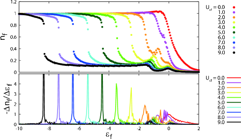
Figure 1: (Upper panel) the $f$-electron number (lower panel) its derivative as a function of the $f$-level at the temperature $T=0.05$ when $U_{cf}=0.0,1.0,\cdots,$ and $9.0$.

When the $f$ level is low enough and the interaction between $f$-electrons is strong enough, the heavy-metallic Kondo state is realized, where $n_{f}\sim 1$. On the other hand, as the $f$ level becomes higher, $n_{f}$ is away from the commensurate value, where the mixed-valence state is realized. It is found that when $U_{cf}=0$, the Kondo state is continuously changed to the mixed-valence state and the crossover occurs around $\epsilon_{f}\sim 0$, where $|\Delta n_{f}/\Delta\epsilon_{f}|$ has maximum. On the other hand, as increasing $U_{cf}$, different behavior appears. The valence at the $f$ level is rapidly changed around the crossover region. Beyond the critical value of $U_{cf}$, the jump singularity appears in the curves, as shown in Fig. 1. This implies the existence of a first-order phase transition between the Kondo and mixed-valence states.

By performing similar calculations, we obtain the finite temperature phase diagram, as shown in Fig. 2.

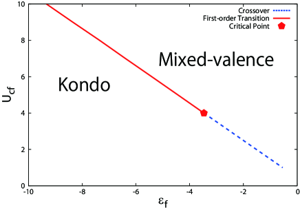
Figure 2: The phase diagram of the extended periodic Anderson model at the temperature $T=0.02$. Solid line represents the phase boundary between the Kondo and mixed-valence regions. Dashed line indicates the crossover between two states.

The Kondo state with $n_{f}\sim 1$ is realized in the case with lower $f$-level. Increasing the $f$ energy level, valence fluctuations are enhanced. In the case $U_{cf}>4$, the first-order valence transition occurs from the Kondo state to the mixed-valence state, while in the other, no sigularity appears in $n_{f}$ and the crossover appears. At the end point of the phase boundary $(U_{cf},\epsilon_{f})\sim(4,-3.7)$, the derivative of the particle number of $f$-electron diverges, where the phase transition is of second order.

Fig. 3 shows the phase diagram in $T-U_{cf}-\epsilon_{f}$ space, by estimating the phase boundaries in the system at different temperatures systematically. At higher temperatures, the effect of the interaction becomes irrelevant and the Kondo state with $n_{f}\sim 1$ becomes unstable. Therefore, the jump singularity in the particle number of $f$-electons smears with increasing temperatures, where the critical end point is shifted up, as shown in Fig. 3. An important point is that the first-order phase boudary between Kondo and mixed-valence regions is little affected by the thermal fluctuation. This implies that at least, in the framework of DMFT with NCA, the valence transition is not induced by lowering temperatures but is induced by changing local parameters $U_{cf}$ and $\epsilon_{f}$.

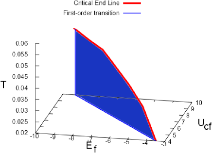
Figure 3: The phase diagram in $T-U_{cf}-\epsilon_{f}$ space.

On the other hand, at low temperatures, the NCA method may not be appropriate to discuss low-energy properties in the system quantitatively. Nevertheless, our results suggests the existence of the quantum critical point at $T=0$, which is consistent with the previous works [6, 7]. Therefore, we have discussed the valence transitions in the extended periodic Anderson model complementally.

4 Summary

We have considered the extended periodic Anderson model by combining dynamical mean-field theory with the non-crossing approximation. Calculating the number of $f$-electrons at each site, we have discussed how valence fluctuations are enhanced by the Coulomb interaction between the conduction and $f$-electrons. We have studied the stability of the valence transition with a jump singularity in the particle number of $f$ electrons at finite temperatures complementally. It is also interesting how the magnetic field induces the metamagnetic transition [8], which is now under consideration.

References

- [1] K. A. Gschneidner and L. Eyring: Handbook on the Physics and Chemistry of rare Earths (North-Holland, Amsterdam, 1978).
- [2] H. Nakamura, K. Nakajima, Y. Kitaoka, K. Asayama, K. Yoshimura, and T. Nitta: J. Phys. Soc. Jpn. 59 (1990) 28.
- [3] B. Kindler, D. Finsterbusch, R. Graf, F. Ritter, W. Assmus, and B. Lüthi: Phys. Rev. B 50 (1994) 704.
- [4] Y. Onishi and K. Miyake: J. Phys. Soc. Jpn. 69 (2000) 3955.
- [5] K. Miyake and H. Maebashi: J. Phys. Soc. Jpn. 71 (2002) 1007.
- [6] S. Watanabe, M. Imada, and K. Miyake: J. Phys. Soc. Jpn. 75 (2006) 043710; S. Watanabe, A. Tsuruta, K. Miyake, and J. Flouquet: Phys. Rev. Lett. 100 (2008) 236401.
- [7] Y. Saiga, T. Sugibayashi, and D. S. Hirashima: J. Phys. Soc. Jpn. 77 (2008) 114710.
- [8] T. Sugibayashi and A. Tsuruta: J. Phys. Soc. Jpn. 79 (2010) 124712.
- [9] W. Metzner and D. Vollhardt: Phys. Rev. Lett. 62 (1989) 324.
- [10] E. Müller-Hartmann: Z. Phys. B: Condens. Matter 74 (1989) 507.
- [11] Th. Pruschke, M. Jarrell, and Freericks: Adv. Phys. 44 (1995) 187.
- [12] A. Georges, G. Kotliar, W. Krauth, and M. J. Rozenberg: Rev. Mod. Phys. 68 (1996) 13.
- [13] G. Kotliar and D. Vollhardt: Phys. Today (2004) 53.
- [14] Y. Kuramoto: Z. Phys. B 53 (1983) 37.
- [15] M. Eckstein and P. Werner: Phys. Rev. B 82 (2010) 115115.
- [16] T. Schork and S. Blawid: Phys. Rev. B 56 (1997) 6559.
- [17] R. Sato, T. Ohashi, A. Koga, and N. Kawakami: J. Phys. Soc. Jpn. 73 (2004) 1864.
- [18] A. Koga, N. Kawakami, R. Peters, and T. Pruschke: Phys. Rev. B 77 (2008) 045120.
- [19] A. Koga, N. Kawakami, R. Peters, and T. Pruschke: J. Phys. Soc. Jpn. 77 (2008) 033704.
- [20] T. Yoshida, T. Ohashi, and N. Kawakami: J. Phys. Soc. Jpn. 80 (2011) 064710.