KUNS-2465
DESY 13-170
More on cosmological constraints on spontaneous R-symmetry breaking models
Yuta Hamada1, Kohei Kamada2,3, Tatsuo Kobayashi1 and Yutaka Ookouchi4
1Department of Physics, Kyoto University, Kyoto 606-8502, Japan
2 Deutsches Elektronen-Synchrotron DESY,
Notkestrasse 85, D-22607 Hamburg, Germany
3Institut de Théorie des Phénomènes Physiques,
École Polytechnique Fédérale de Lausanne,
CH-1015 Lausanne, Switzerland
4Faculty of Arts and Science, Kyushu
University, Fukuoka 819-0395, Japan
Abstract
We study the spontaneous R-symmetry breaking model and investigate the cosmological constraints on this model due to the pseudo Nambu-Goldstone boson, R-axion. We consider the R-axion which has relatively heavy mass in order to complement our previous work. In this regime, model parameters, R-axions mass and R-symmetry breaking scale, are constrained by Big Bang Nucleosynthesis and overproduction of the gravitino produced from R-axion decay and thermal plasma. We find that the allowed parameter space is very small for high reheating temperature. For low reheating temperature, the breaking scale is constrained as regardless of the value of R-axion mass.
1 Introduction
Supersymmetry (SUSY) is one of the most promising candidates of the physics beyond the standard model (SM) because it can relax the naturalness problem and suggests the gauge coupling unification. It is also widely believed to be one of the key ingredients for constructing a consistent string theory encompassing the SM. Since SUSY has not been observed in experiments yet, it has to be broken somewhere between the weak scale and the Planck scale. Recent discovery of a Higgs boson at the LHC [1] may suggest that the stop mass is around TeV without introducing an artificial new mechanism [2], in particular, in models of gauge mediation, which is the main topic in this paper. Although it is not at the right scale for solving the naturalness problem,111In a certain scenario, a heavy stop mass such as several TeV is still natural [3]. other good points of SUSY encourage us to study it further. Therefore, we focus on relatively high-scale SUSY-breaking scenarios in this paper.
If high-scale SUSY is realized in nature, it would be interesting to seek for a connection between the SUSY breaking scale and cosmological observations, which are quite useful tools to probe the high-scale physics beyond the TeV scale. Among many other scenarios of high-scale SUSY breaking, gauge mediation models with spontaneously broken R-symmetry, which is a specific symmetry in supersymmetric theories, is one of the models that has recently experienced striking progress on model building [4], (see for reviews [5, 6, 7]). As is emphasized in Refs. [8, 9, 10, 11], R-symmetry opens up interesting windows into the connection between SUSY breaking and cosmological aspects. In particular, cosmology with the Nambu-Goldstone boson, called R-axion, which is generated and acquires a mass term in coupling to the gravity theory because the constant term in superpotential breaks R-symmetry explicitly is an interesting working place; R-axions are produced at some time in the cosmic history and their decays may affect the standard cosmological scenario, which, in turn, constrains the model parameters [8].
Depending on its mass scale, various decay modes are allowed. In our previous study [8], we focused on relatively light and long-lived R-axions since such parameter regions are favored in the context of “low-scale gauge mediation” [12], where various cosmological constraints including the Big Bang Nucleosynthesis (BBN), the Cosmic Microwave Background (CMB), cosmic -ray and the re-ionization can be imposed in the late epoch of the expanding universe. In addition to these constraints, we here point out that the abundance of heavier R-axions with shorter lifetime, which can explain the 125 GeV Higgs more easily, can be constrained in a wide range of parameter space by two cosmological constraints: One is coming from hadronic decays of R-axions. When the mass scale of the R-axion is much larger than GeV, the R-axion can efficiently decay into various hadrons. For sufficiently heavy R-axions, they immediately turn to hadronic jets, which affects successful BBN. This phenomenon can constrain the parameter space of R-axions. The other constraint comes from gravitino production. In this short note, we mainly focus on the regime in which gauge mediation is the dominant contribution to the mediation of SUSY breaking. In this case, the gravitino is a stable particle and can be over-produced via R-axion decay. In fact, as we will show below, overproduction of such gravitinos yields a condition which is complementary to the one for thermal production of gravitino.
In this paper, we investigate cosmological effects of heavy R-axion whose mass scale is not covered in the previous work [8]. Especially, we focus the mass scale heavier than to avoid subtlety of non-relativistic decay into pions which requires careful treatment because it does not necessarily destroy the light elements constructed by BBN. Also, we assume that all superparticles (except gravitino) are heavier than the R-axion because R-axion decay into superparticles requires highly model dependent argument. If the decay channel into superparticles of R-axions opens, the constraint would become more severe.
The organization of this paper is as follows: In section 2, we briefly review the R-symmetry breaking model. Then, we examine the lifetime of the R-axion and the branching ratio of hadronic decays. In section 3, we firstly review the mechanisms of the R-axion production and its abundance. Then we impose constraints on R-axion abundance from the BBN and gravitino overproduction. As we will show that the R-axion mass and R-symmetry breaking scale are severely constrained. Section 4 is devoted to summary and discussion.
2 Hadronic decay of R-axion
In this section, we briefly review the simple model with spontaneously broken R-symmetry studied in Ref. [8]. Let us focus on the R-charged light SUSY-breaking field, , and consider a low-energy scale where all other fields including messenger fields are integrated out. The effective superpotential is, then, assumed to be
| (2.1) |
Here the constant term is required to realize vanishing cosmological constant. Note that this class of models is common in various -term supersymmetry breaking models [4]. We assume non-canonical Kähler potential yielding the following potential,
| (2.2) |
which realizes a potential minimum with spontaneously broken R-symmetry. Here is the reduced Planck mass. The first term comes from our assumption about Kähler potential. is turned out to be the “axion decay constant” and we assume . The second term appears from the Planck-suppressed interaction in supergravity theory. It breaks R-symmetry explicitly and generates the mass term for the R-axion, the phase component of the field. In coupling to the gravity, vanishing cosmological constant requires
| (2.3) |
Though we have introduced an ad-hoc Kähler potential for the SUSY-braking vacuum with spontaneously broken R-symmetry, we believe that it is a simple toy model which reveals various aspects in spontaneous R-symmetry breaking models 222As we will see later, in order to put cosmological constraints, we need to know the interactions and the abundance of R-axions. In spontaneous R-symmetry breaking models, these are characterized by R-axion mass and decay constant for any Kähler potential. Therefore, taking and as free parameters, our discussion of ad-hoc Kähler potential is applicable to many spontaneous R-symmetry breaking models where the R-symmetry breaking is realized by general non-canonical Kähler potential. [4]. Dividing into VEV and fluctuation,
| (2.4) |
we have the potential for and as
| (2.5) |
Hereafter we call R-saxion and R-axion. From the potential, we can read off the R-axion mass and R-saxion mass as
| (2.6) |
We expect that R-symmetry breaking potential Eq.(2.2) would be related to SUSY breaking and
| (2.7) |
With this assumption, we find the relation of and as
| (2.8) |
Meanwhile the gravitino mass is written by
| (2.9) |
Since the gravitino is lighter than R-axion while R-saxion is heavier than R-axion, R-axion can decay into gravitinos but not R-saxions.
Now we evaluate the interactions of R-axions, which is necessary to investigate the production and decay rate of R-axions. First, let us consider the interaction with the gauge fields. R-axions couple with the SM gauge fields through anomaly couplings,
| (2.10) |
where for and 1 represent the SM gauge groups , and , respectively and s are the corresponding gauge couplings. From these couplings, we obtain the decay rates of R-axion to each pair of gauge bosons as
| (2.11) |
where is the Weinberg angle and and are the Z-boson and W-boson masses, respectively. Since the anomaly coefficients are model-dependent parameters of the order of the unity, we take for all in the following. Taking other values of the order of the unity does not change our results significantly.
Secondly, the R-axion can also couple with the SM fermions through the mixing between the R-axion and the Higgs bosons [12]. Couplings with up type quarks, down type quarks, charged leptons and neutrinos are expressed as the effective interactions, with the coupling constants
| (2.12) |
where with and denotes the mass of each fermion . is the ratio of the vacuum expectation values of the up-type Higgs boson and the down-type Higgs boson . From these couplings, R-axions can decay into a pair of fermions with the decay rates,
| (2.15) |
Note that as well as other parameters such as the stop mass determines the Higgs mass. For the 125 GeV Higgs, is favored for the stop mass with a few TeV [2].
Finally, R-axions can decay to a pair of gravitinos through supergravity effect,
| (2.16) |
Decay rate is given by
| (2.17) |
for . Here we have used the relation and taken into account that for the light gravitino, the decay into the spin 1/2 goldstino component with dominates over the decay into the spin 3/2 component [13].
We plot the lifetime of the R-axion for in Fig.-179. For , decay into tau pairs dominates; for , decay into bottom pairs dominates; and for , decay into gluon or gravitino pairs dominates. Note that for large , the decaying into the gravitino pairs dominates other channels for the heavy R-axion mass since the suppression factor is not so small that overwhelms the loop factors. From this figure, We can see that the lifetime is shorter than s for .
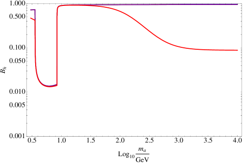
In the case that the energy injected quarks are high enough, right after the axion decay, quarks and gluons immediately turn into hadronic jets333 If the axion mass is around GeV, axion dominantly decay into non- or semi-relativistic pions. In this case the detail of the decay process matters and the analysis is subtle and complicated, and hence we do not consider such cases.. Hence, the process does not depend on the first particles created by axion decay. For the BBN constraint, then, only the branching ratio decaying into hadronic particles determines the constraint. We present the hadronic branching ratio of the R-axion for in Fig.-178, where is the sum of the branching ratio of the R-axion to colored particles. becomes small if we take larger since the branching ratio of the R-axion decay into gravitinos becomes sizable. It is found that becomes constant for large , . Numerically is of for . For , decay channel into bottom pairs dominates the total decaying ratio, we have regardless of . For , becomes small once more because the decay channel to taus dominates the total decay ratio. In this range is of . Summarizing the above, is bigger than for . Thus, the constraint with gives the stringent constraint whereas that with gives the conservative one, as we will see in the next section.

3 Cosmological constraints on R-axion abundance
3.1 R-axion production
Let us consider the R-axion cosmology. First we study the R-axion production. The R-axion production depends on cosmological scenarios, and we here simply suppose that the breaking occurs after inflation. In this case, cosmic R-string forms at the time of the phase transition [9]. The cosmic R-strings enter the scaling regime quickly, and the cosmic string loops that are produced continuously emit R-axions, which is the first source of R-axions [14]. Gradually the explicit breaking effect can no longer be neglected, and string network turns into string-wall system, which is unstable and decay to R-axions immediately [15]. This is the second source of R-axions. At the same time, coherent oscillation of R-axions also starts, which is the third source of R-axions [16]. In addition to these R-axion production from the dynamics, there are thermal production [17] and production from R-saxion decay of R-axions. Note that it can be shown that production from R-saxion decay is negligible (see Appendix of Ref. [8]). Here we summarize the R-axion production from the dynamics (the coherent oscillation, the decay of cosmic string, decay of the string-wall system) and thermal bath referring the result of Ref. [8]. The R-axion abundance produced from dynamics is given by
| (3.3) |
where is reheating temperature. and are Hubble parameters evaluated at the time of reheating and of beginning of the R-axion oscillation, respectively. Note that the result changes only by numerical factors, but parameter dependence does not change if we consider the scenario without cosmic string formation but only with the coherent oscillation of R-axion [8]. The abundance of R-axions produced thermally is given by
| (3.6) |
where is the decoupling temperature. This value is fixed when R-axions become non relativistic. Note that for , R-axions are once thermalized and the R-axion abundance becomes independent of the reheating temperature.
3.2 Constraints for parameter space
The standard BBN scenario can explain the light elements in the present Universe elegantly. However, if massive exotic particle decays occur during or after BBN epoch, light elements would be broken by the decay products, which would abandon the successful BBN [18, 19]. In particular, if the decay includes hadronic decay with hadronic jets, a lot of 4He’s are destroyed and 3He, D, and T are produced from 4He dissociation, which gives much stringent constraint. Hence the amount of hadronic decay product must be small enough, and in turn, R-axion abundance is constrained. The abundance of R-axions is constrained with respect to their decay rate and hadronic branching ratio. For , this constraint [19] is given by
| (3.13) |
The constraint for [19] is also given by
| (3.22) |
Since we have seen from Fig. -178, we obtain the conservative bound if we use (3.13). The larger is, the more severe constraint becomes. Then, (3.22) for gives more severe bound than (3.13). Note that is the good approximation for and . Later, we will show the results of both cases.
There is another cosmological constraint on the R-axion abundance. Since R-axions can decay into the stable gravitinos, their abundance from R-axion decay may overwhelm the present abundance of dark matter (DM). Since the gravitino abundance should not exceed that of DM, we have the following constraint as
| (3.23) |
where is branching ratio of gravitino. Note that the present gravitino abundance has a suppression factor , since a R-axion decays into two relativistic gravitinos with the total energy and gradually becomes nonrelativistic. Since this constraint comes from the present Universe, it exists regardless of the lifetime of R-axion if .
We should also note the constraint from the gravitino produced thermally. The thermally produced gravitino abundance is given by [21]
| (3.24) |
which must be smaller than, again, , where is the gluino mass. Therefore, we need relatively large gravitino mass to avoid the overclosure problem, depending on the gravitino mass. In other words, relatively large and are required, see Eq. (2.9).

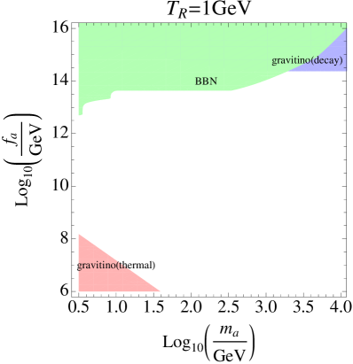
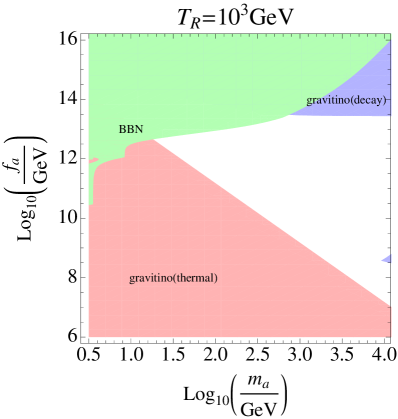
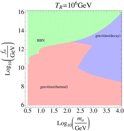
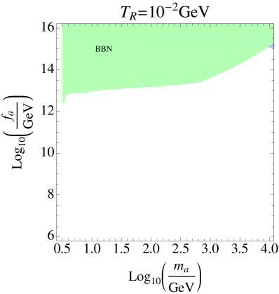
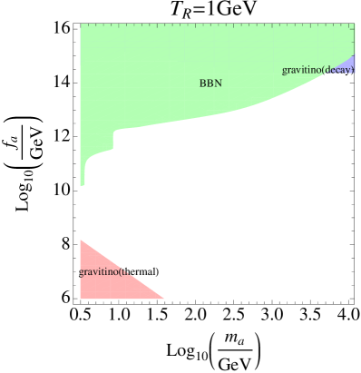
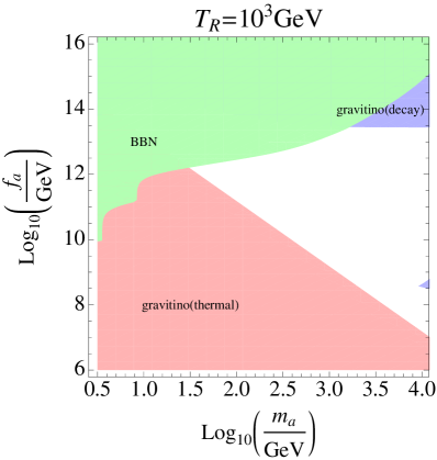
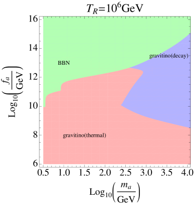
In Fig. -177 and Fig. -176, we present the cosmological constraints on model parameters discussed above, in terms of and with various cases of the reheating temperature. Here we have set . If the reheating temperature is high, GeV, thermal production of R-axion is so large that the gravitino abundance from the R-axion decay exceeds that of DM for GeV and GeV. Since the gravitinos produced thermally overclose the Universe for light gravitinos, which means small and , the allowed parameter space is very small. Allowed parameter region enlarges for lower reheating temperature. In particular, the gravitino overclosure problem is almost absent for GeV. In this case, model parameters are constrained only by the BBN. We can see that R-symmetry breaking scale is constrained from above regardless of the reheating temperature, . Note that we find that the constraint would not change so much if we use the precise value of (between to 1) by comparing the constraints of and .
We comment on the generality of the constraints shown in Fig. -177 and Fig. -176. R-axions couple with SM gauge fields through anomaly couplings and couple with the SM fermions through the mixing between the R-axion and the Higgs bosons which comes from B-term in Higgs potential. These couplings are general in spontaneous R-symmetry breaking models up to numerical factor. On the other hand, it would be possible to change the gravitino mass relation Eq. (2.9) and the R-axion gravitino coupling Eq. (2.17) if we consider more complicated superpotential. In order to avoid the constraint from gravitinos, we need a model to change Eq. (2.9) or Eq. (2.17).
It would be interesting to further explore heavier R-axion such as TeV. In this case, various decay modes into superparticles are open. Thus, arguments become highly model dependent. We will study some examples elsewhere.
4 Summary and discussions
In this paper, we considered the spontaneous R-symmetry breaking model and investigated the cosmological constraints of heavy R-axion which can decay to hadrons. This work complements our previous one [8]. We estimated the abundance of the R-axion produced by decay of R-string and domain wall, vacuum misalignment and thermal plasma. Such abundance is constrained by BBN and the gravitino overproduction. We showed cosmological constraints on model parameters, R-axion mass and R-symmetry breaking scale. As a result, we found that breaking scale is constrained as GeV for low reheating temperature regardless of the value of R-axion mass. For high reheating temperature, BBN, gravitinos from R-axion decay, and gravitinos from thermal plasma constrain different parameter regions and the allowed parameter space is very small. In conclusion, even in the heavy R-axion regime, it has poor compatibility with relatively high reheating temperature GeV. The constraints we showed in this paper can apply to many spontaneous R-symmetry breaking models and are important for phenomenological model building.
Finially it would be useful to re-interpret out results shown above as a constraint for messenger scale by using a simple gauge mediation model, taking the following simple messenger sector,
| (4.1) |
where and represent messenger fields. In this set up, the stop mass is given by
| (4.2) |
In the second line, we used Eq.(2.6) and Eq.(2.8). From this expression we obtain the following formula,
| (4.3) |
In order to realize the appropriate Higgs mass, we take [20]. Therefore, from Eq.(4.3) is required for to obtain .
Acknowledgment
The authors would like to thank M. Ibe for useful comments and discussions. Especially, we would like to thank K. Kohri for his lectures on the Big Bang Nucleosynthesis and for crucial comments on hadronic decay of R-axion. The work of Y. H. was supported by a Grant-in-Aid for Japan Society for the Promotion of Science (JSPS) Fellows No.251107. T.K. is supported in part by the Grants-in-Aid for Scientific Research (A) No. 22244030 and 25400252 from the Ministry of Education, Culture,Sports, Science and Technology of Japan. The work of YO is supported by Grant-in-Aid for Scientific Research from the Ministry of Education, Culture, Sports, Science and Technology, Japan (No. 25800144 and No. 25105011). The work of KK is supported by a JSPS postdoctoral fellowship for research abroad.
References
- [1] G. Aad et al. [ATLAS Collaboration], Phys. Lett. B 716, 1 (2012) [arXiv:1207.7214 [hep-ex]]; S. Chatrchyan et al. [CMS Collaboration], Phys. Lett. B 716, 30 (2012) [arXiv:1207.7235 [hep-ex]].
- [2] P. Draper, P. Meade, M. Reece and D. Shih, Phys. Rev. D 85, 095007 (2012) [arXiv:1112.3068 [hep-ph]]; M. Ibe, S. Matsumoto and T. T. Yanagida, Phys. Rev. D 85, 095011 (2012) [arXiv:1202.2253 [hep-ph]]; B. Bhattacherjee, B. Feldstein, M. Ibe, S. Matsumoto and T. T. Yanagida, arXiv:1207.5453 [hep-ph]; T. Higaki, K. Kamada and F. Takahashi, JHEP 1209, 043 (2012) [arXiv:1207.2771 [hep-ph]]; B. Feldstein and T. T. Yanagida, arXiv:1210.7578 [hep-ph]; T. Moroi, T. T. Yanagida and N. Yokozaki, arXiv:1211.4676 [hep-ph]; M. Endo, K. Hamaguchi, S. Iwamoto and N. Yokozaki, JHEP 1206, 060 (2012) [arXiv:1202.2751 [hep-ph]].
- [3] K. Choi, K. S. Jeong, T. Kobayashi and K. -i. Okumura, Phys. Lett. B 633, 355 (2006) [hep-ph/0508029]; R. Kitano and Y. Nomura, Phys. Lett. B 631, 58 (2005) [hep-ph/0509039]; K. Choi, K. S. Jeong, T. Kobayashi and K. -i. Okumura, Phys. Rev. D 75, 095012 (2007) [hep-ph/0612258]; T. Kobayashi, H. Makino, K. -i. Okumura, T. Shimomura and T. Takahashi, JHEP 1301, 081 (2013) [arXiv:1204.3561 [hep-ph]].
- [4] D. Shih, JHEP 0802, 091 (2008) [hep-th/0703196]; C. Cheung, A. L. Fitzpatrick and D. Shih, JHEP 0807, 054 (2008) [arXiv:0710.3585 [hep-ph]]; L. Ferretti, JHEP 0712, 064 (2007) [arXiv:0705.1959 [hep-th]]; H. Y. Cho and J. -C. Park, JHEP 0709, 122 (2007) [arXiv:0707.0716 [hep-ph]]; S. Abel, C. Durnford, J. Jaeckel and V. V. Khoze, Phys. Lett. B 661, 201 (2008) [arXiv:0707.2958 [hep-ph]]; L. G. Aldrovandi and D. Marques, JHEP 0805, 022 (2008) [arXiv:0803.4163 [hep-th]]; L. M. Carpenter, M. Dine, G. Festuccia and J. D. Mason, Phys. Rev. D 79, 035002 (2009) [arXiv:0805.2944 [hep-ph]]; A. Giveon, A. Katz, Z. Komargodski and D. Shih, JHEP 0810, 092 (2008) [arXiv:0808.2901 [hep-th]]; Z. Sun, JHEP 0901, 002 (2009) [arXiv:0810.0477 [hep-th]]; Z. Komargodski and D. Shih, JHEP 0904, 093 (2009) [arXiv:0902.0030 [hep-th]]; J. L. Evans, M. Ibe, M. Sudano and T. T. Yanagida, JHEP 1203, 004 (2012) [arXiv:1103.4549 [hep-ph]]; T. Azeyanagi, T. Kobayashi, A. Ogasahara and K. Yoshioka, Phys. Rev. D 86, 095026 (2012) [arXiv:1208.0796 [hep-ph]].
- [5] K. A. Intriligator and N. Seiberg, Class. Quant. Grav. 24, S741 (2007) [hep-ph/0702069].
- [6] R. Kitano, H. Ooguri and Y. Ookouchi, Ann. Rev. Nucl. Part. Sci. 60, 491 (2010) [arXiv:1001.4535 [hep-th]].
- [7] M. Dine and J. D. Mason, Rept. Prog. Phys. 74, 056201 (2011) [arXiv:1012.2836 [hep-th]].
- [8] Y. Hamada, K. Kamada, T. Kobayashi and Y. Ookouchi, JCAP 1304 (2013) 043 [arXiv:1211.5662 [hep-ph]].
- [9] M. Eto, Y. Hamada, K. Kamada, T. Kobayashi, K. Ohashi and Y. Ookouchi, JHEP 1303 (2013) 159 [arXiv:1211.7237 [hep-th]].
- [10] K. Kamada, T. Kobayashi, K. Ohashi and Y. Ookouchi, JHEP 1305, 091 (2013) [arXiv:1303.2740 [hep-ph]].
- [11] T. Hiramatsu, M. Eto, K. Kamada, T. Kobayashi and Y. Ookouchi, arXiv:1304.0623 [hep-ph].
- [12] H. -S. Goh and M. Ibe, JHEP 0903 (2009) 049 [arXiv:0810.5773 [hep-ph]].
- [13] T. Moroi, hep-ph/9503210.
- [14] R. L. Davis, Phys. Lett. B 180, 225 (1986); A. Vilenkin and T. Vachaspati, Phys. Rev. D 35, 1138 (1987); R. A. Battye and E. P. S. Shellard, Nucl. Phys. B 423, 260 (1994) [astro-ph/9311017]; M. Yamaguchi, M. Kawasaki and J. ’i. Yokoyama, Phys. Rev. Lett. 82, 4578 (1999) [hep-ph/9811311]; T. Hiramatsu, M. Kawasaki, T. Sekiguchi, M. Yamaguchi and J. ’i. Yokoyama, Phys. Rev. D 83, 123531 (2011) [arXiv:1012.5502 [hep-ph]].
- [15] P. Sikivie, Phys. Rev. Lett. 48, 1156 (1982); D. H. Lyth, Phys. Lett. B 275, 279 (1992); M. Nagasawa and M. Kawasaki, Phys. Rev. D 50, 4821 (1994) [astro-ph/9402066]; S. Chang, C. Hagmann and P. Sikivie, Phys. Rev. D 59, 023505 (1999) [hep-ph/9807374]; T. Hiramatsu, M. Kawasaki, K. ’i. Saikawa and T. Sekiguchi, Phys. Rev. D 85, 105020 (2012) [Erratum-ibid. D 86, 089902 (2012)] [arXiv:1202.5851 [hep-ph]].
- [16] J. Preskill, M. B. Wise and F. Wilczek, Phys. Lett. B 120, 127 (1983); L. F. Abbott and P. Sikivie, Phys. Lett. B 120, 133 (1983); M. Dine and W. Fischler, Phys. Lett. B 120, 137 (1983);
-
[17]
E. Masso, F. Rota and G. Zsembinszki,
Phys. Rev. D 66, 023004 (2002) [hep-ph/0203221].
P. Sikivie, Lect. Notes Phys. 741, 19 (2008) [astro-ph/0610440].
P. Graf and F. D. Steffen, Phys. Rev. D 83, 075011 (2011) [arXiv:1008.4528 [hep-ph]]. - [18] M. H. Reno and D. Seckel, Phys. Rev. D 37 (1988) 3441.
- [19] M. Kawasaki, K. Kohri and T. Moroi, Phys. Rev. D 71 (2005) 083502 [astro-ph/0408426].
- [20] J. L. Feng, P. Kant, S. Profumo and D. Sanford, arXiv:1306.2318 [hep-ph].
- [21] M. Bolz, A. Brandenburg and W. Buchmuller, Nucl. Phys. B 606, 518 (2001) [Erratum-ibid. B 790, 336 (2008)] [hep-ph/0012052]; M. Endo, F. Takahashi and T. T. Yanagida, Phys. Rev. D 76, 083509 (2007) [arXiv:0706.0986 [hep-ph]].