Spectra of random graphs with community structure and arbitrary degrees

Abstract

Using methods from random matrix theory researchers have recently calculated the full spectra of random networks with arbitrary degrees and with community structure. Both reveal interesting spectral features, including deviations from the Wigner semicircle distribution and phase transitions in the spectra of community structured networks. In this paper we generalize both calculations, giving a prescription for calculating the spectrum of a network with both community structure and an arbitrary degree distribution. In general the spectrum has two parts, a continuous spectral band, which can depart strongly from the classic semicircle form, and a set of outlying eigenvalues that indicate the presence of communities.

I Introduction

Spectral analysis of networks provides a useful complement to traditional analyses that focus on local network properties like degree distributions, correlation functions, or subgraph densities Newman03d ; Boccaletti06 . Spectral analysis can return nonlocal information about network structure such as optimal partitions Fiedler73 ; PSL90 , community structure Newman06c , and nonlocal centrality measures Bonacich87 and has been widely used in the study of real-world network data since the 1970s. In additional to the development of practical algorithms and methods based on network spectra, such as spectral partitioning schemes and community detection algorithms, a considerable amount of work has been done on the analytic calculation of spectra for synthetic networks generated using random models FDBV01 ; GKK01a ; CLV03 ; DGMS03 ; Kuhn08 ; CGO09 ; NN12 ; NN13 . Study of these model networks can help us to understand how particular features of network structure are reflected in spectra and to anticipate the performance of spectral algorithms.

Recent work on the spectra of networks with community structure, for instance, has demonstrated the presence of a “detectability threshold” as a function of the strength of the embedded structure NN12 . When the community structure becomes sufficiently weak it can be shown that the spectrum loses all trace of that structure, implying that any method or algorithm for community detection based on spectral properties must fail at this transition point. A limitation of this work, however, is that the synthetic networks studied have Poisson degree distributions, which makes the calculations easier but is known to be highly unrealistic; real-world degree distributions are very far from Poissonian.

In other work a number of authors have studied the spectra of synthetic networks having broad degree distributions, such as the power-law distributions observed in many real-world networks FDBV01 ; GKK01a ; CLV03 ; DGMS03 ; Kuhn08 ; NN13 . Among other results, it is found that while the spectrum for Poisson degree distributions follows the classic Wigner semicircle law, in the more general case it departs from the semicircle, sometimes dramatically.

In this paper, we combine these two previous lines of investigation and study the spectra of networks that possess general degree distributions and simultaneously contain community structure. To do this, we make use of a recently proposed network model that generalizes the models studied before. We derive an analytic prescription for calculating the adjacency matrix spectra of networks generated by this model, which is exact in the limit of large network size and large average degree. In general the spectra have two components. The first is a continuous spectral band containing most of the eigenvalues but having a shape that deviates from the semicircle law seen in networks with Poisson degree distribution. The second component consists of outlying eigenvalues, outside the spectral band and normally equal in number to the number of communities in the network.

II The model

The previous calculations described in the introduction make use of two classes of model networks. For networks with community structure, calculations were performed using the stochastic block model, in which vertices are divided into groups and edges placed between them independently at random with probabilities that depend on the group membership of the vertices involved HLL83 ; CK01 ; RL08 ; DKMZ11a ; NN12 ; HRN12 . This model gives community structure of tunable strength but vertices have a Poisson distribution of degrees within each community.

For networks without community structure but with non-Poisson degree distributions, most calculations have been performed using the so-called configuration model, a random graph conditioned on the actual degrees of the vertices MR95 ; NSW01 , or a variant of the configuration model in which one fixes only the expected values of the degrees and not their actual values CL02b .

The calculations presented in this paper make use of a model proposed by Ball et al. BKN11 that simultaneously generalizes both the stochastic block model and the configuration model, so that both are special cases of the more general model. The model of Ball et al. is defined as follows. We assume an undirected network of $n$ vertices labeled $i=1\ldots n$, with each of which is associated a $q$-component real vector $\mathbf{k}_{i}$ where $q$ is a parameter we choose. Then the number of edges between vertices $i$ and $j$ is an independent, Poisson-distributed random variable with mean $\mathbf{k}_{i}\!\cdot\!\mathbf{k}_{j}/2m$, where $m$ is a normalizing constant given by

$$2m=\Biggl{|}\,\sum_{i=1}^{n}\mathbf{k}_{i}\Biggr{|}.$$ (1)

Physically the value of $m$ represents the average total number of edges in the whole network. Its inclusion is merely conventional—one could easily omit it and renormalize $\mathbf{k}_{i}$ accordingly, and in fact Ball et al. did omit it in their original formulation of the model. However, including it will simplify our notation later, as well as making the connection between this model and the configuration model clearer.

The expected number of edges between vertices must be non-negative and Ball et al. ensured this by requiring that the elements of the vectors $\mathbf{k}_{i}$ all be non-negative, but this is not strictly necessary since one can always rotate the vectors globally through any angle (thereby potentially introducing some negative elements) without affecting their products $\mathbf{k}_{i}\!\cdot\!\mathbf{k}_{j}$. In this paper we will only require that all products be nonnegative, which includes all cases studied by Ball et al. but also allows us to consider some cases they did not.

Note that it is possible in this model for there to be more than one edge between any pair of vertices (because the number of edges is Poisson distributed) and this may seem unrealistic, but in almost all real-world situations we are concerned with networks that are sparse, in the sense that only a vanishing fraction of all possible edges is present in the network, which means that $\mathbf{k}_{i}\cdot\mathbf{k}_{j}/2m$ will be vanishing as $n$ becomes large. We will assume this to be the case here, in which case the chances of having two or more edges between the same pair of vertices also vanishes and for practical purposes the network contains only single edges.

The average degree $c$ of a vertex in the network is

$$c={2m\over n}=\biggl{|}{1\over n}\sum_{i=1}^{n}\mathbf{k}_{i}\biggr{|},$$ (2)

and hence increases in proportion to the average of $\mathbf{k}_{i}$. In this paper we will consider networks where the vectors $\mathbf{k}_{i}$ can have a completely general distribution, which gives us a good deal of flexibility about the structure of our network, but consider for example a network in which the vectors have arbitrary lengths, but each one points toward one of the corners of a regular $q$-simplex in a (hyper)plane perpendicular to the direction $(1,1,1,\ldots)$. For such a choice the vectors have the form $\mathbf{k}_{i}=k_{i}\mathbf{v}_{r}$, where $k_{i}$ is the magnitude of the vector and $\mathbf{v}_{r}$ is one of $q$ unit vectors that will denote the group $r$ that vertex $i$ belongs to. Then

$$\mathbf{k}_{i}\!\cdot\!\mathbf{k}_{j}=k_{i}k_{j}\mathbf{v}_{r}\!\cdot\!\mathbf{v}_{s}=k_{i}k_{j}[\delta_{rs}+(1-\delta_{rs})\cos\phi],$$ (3)

where $\phi$ is the angle between unit vectors $\mathbf{v}_{r}$ and $\mathbf{v}_{s}$ (all vectors being separated by the same angle in a regular simplex). Thus for this choice of parametrization we can increase the expected number of edges from $i$ to all other vertices by increasing the magnitude $k_{i}$ of the vector $\mathbf{k}_{i}$, hence increasing the vertex’s degree. At the same time we can independently control the relative probability of connections within groups (when $r=s$) and between them ($r\neq s$) by varying the angle $\phi$.

If we set $\phi=0$ (so that all $\mathbf{v}_{r}$ point in the $(1,1,1,\ldots)$ direction) then this model becomes equivalent to the variant of the configuration model in which the expected vertex degrees are fixed and there is probability $k_{i}k_{j}/2m$ of connection between each pair of vertices, regardless of community membership. (Alternatively, if we set the number of groups $q$ to 1, so that the vectors $\mathbf{k}_{i}$ become scalars $k_{i}$ then we also recover the configuration model.) If we allow $\phi$ to be nonzero but make all $k_{i}$ equal to the same constant value $a$, then the model becomes equivalent to the standard stochastic block model, having a probability $p_{\textrm{in}}=a^{2}/2m$ of connection between vertices in the same community and a smaller probability $p_{\textrm{out}}=(a^{2}/2m)\cos\phi$ between vertices in different communities. For all other choices, the model generalizes both the configuration model and the stochastic block model, allowing us to have nontrivial degrees and community structure in the same network, as well as other more complex types of structure (such as overlapping groups—see Ref. BKN11 ).

III Calculation of the spectrum

In this section we calculate the average spectrum of the adjacency matrix $\mathbf{A}$ for networks generated from the model above, in the limit of large system size. The adjacency matrix is the symmetric matrix with elements $A_{ij}$ equal to the number of edges between vertices $i$ and $j$. The elements are Poisson independent random integers for our model, although crucially they are not identically distributed. The spectra of matrices with Poisson elements of this kind can be calculated using methods of random matrix theory. Our strategy will be first to calculate the spectrum of the matrix

$$\mathbf{X}=\mathbf{A}-\langle\mathbf{A}\rangle,$$ (4)

where $\langle\mathbf{A}\rangle$ is the average value of the adjacency matrix within the model, which has elements $\langle A_{ij}\rangle=\mathbf{k}_{i}\!\cdot\!\mathbf{k}_{j}/2m$. Since $\mathbf{k}_{i}$ is a $q$-element vector, this implies that $\langle\mathbf{A}\rangle$ has rank $q$ and hence its eigenvector decomposition has the form

$$\langle\mathbf{A}\rangle=\sum_{r=1}^{q}\alpha_{r}\mathbf{u}_{r}\mathbf{u}_{r}^{T},$$ (5)

where $\mathbf{u}$ are normalized eigenvectors and $\alpha_{r}$ are the corresponding eigenvalues.

The matrix $\mathbf{X}$ is a “centered” random matrix, having independent random elements with zero mean, which makes the calculation of its spectrum particularly straightforward. Once we have calculated the spectrum of this centered matrix we will then add the rank-$q$ term $\langle\mathbf{A}\rangle$ back in as a perturbation:

$$\mathbf{A}=\mathbf{X}+\langle\mathbf{A}\rangle.$$ (6)

As we will see, the only property of the centered matrix needed to compute its spectrum is the variance of its elements, and since the variance of a Poisson distribution is equal to its mean, we can immediately deduce that the variance of the $ij$ element of $\mathbf{X}$ is $\mathbf{k}_{i}\!\cdot\!\mathbf{k}_{j}/2m$.

III.1 Spectrum of the centered matrix

In this section we calculate the spectral density $\rho(z)$ of the centered matrix $\mathbf{X}$, Eq. (4). The spectral density is defined by

$$\rho(z)={1\over n}\sum_{i=1}^{n}\delta(z-\lambda_{i}),$$ (7)

where $\lambda_{i}$ is the $i$th eigenvalue of $\mathbf{X}$ and $\delta(z)$ is the Dirac delta. The starting point for our calculation is the well-known Stieltjes–Perron formula, which gives the spectral density directly in terms of the matrix as

$$\rho(z)=-{1\over n\pi}\operatorname{Im}\operatorname{Tr}\bigl{\langle}(z-\mathbf{X})^{-1}\bigr{\rangle},$$ (8)

where $z-\mathbf{X}$ is shorthand for $z\mathbf{I}-\mathbf{X}$ with $\mathbf{I}$ being the identity.

To calculate the trace, we follow the approach of Bai and Silverstein BS10 , making use of the result that the $i$th diagonal component of the inverse of a symmetric matrix $\mathbf{B}$ is NN13

$$\bigl{[}\mathbf{B}^{-1}\bigr{]}_{ii}={1\over B_{ii}-\mathbf{b}_{i}^{T}\mathbf{B}_{i}^{-1}\mathbf{b}_{i}},$$ (9)

where $B_{ii}$ is the $i$th diagonal element of $\mathbf{B}$, $\mathbf{b}_{i}$ is the $i$th column of the matrix, and $\mathbf{B}_{i}$ is the matrix with the $i$th row and column removed. In the limit of large system size, and provided that the degrees of vertices become large as the network does, the distribution of values of $[\mathbf{B}^{-1}]_{ii}$ becomes narrowly peaked about its mean, and one can write the mean value as

$$\bigl{\langle}\bigl{[}\mathbf{B}^{-1}\bigr{]}_{ii}\bigr{\rangle}={1\over\langle B_{ii}\rangle-\langle\mathbf{b}_{i}^{T}\mathbf{B}_{i}^{-1}\mathbf{b}_{i}\rangle}.$$ (10)

If, as in our case, the elements of $\mathbf{B}$ are independent random variables with mean zero, then

$$\bigl{\langle}\mathbf{b}_{i}^{T}\mathbf{B}_{i}^{-1}\mathbf{b}_{i}\bigr{\rangle} =\sum_{jk}\bigl{\langle}\bigl{[}\mathbf{B}_{i}^{-1}\bigr{]}_{jk}\bigr{\rangle}\bigl{\langle}[\mathbf{b}_{i}]_{j}[\mathbf{b}_{i}]_{k}\bigr{\rangle}$$

$$=\sum_{j}\bigl{\langle}\bigl{[}\mathbf{B}_{i}^{-1}\bigr{]}_{jj}\bigr{\rangle}\bigl{\langle}[\mathbf{b}_{i}]_{j}^{2}\bigr{\rangle},$$ (11)

where we have made use of $\langle[\mathbf{b}_{i}]_{j}[\mathbf{b}_{i}]_{k}\rangle=\langle[\mathbf{b}_{i}]_{j}\rangle\langle[\mathbf{b}_{i}]_{k}\rangle=0$ when $j\neq k$.

In our particular example we have $\mathbf{B}=z-\mathbf{X}$, which means that

$$[\mathbf{b}_{i}]_{j}=-X_{ij}$$ (12)

(since $i\neq j$ by definition, the $i$th row having been removed from the matrix), so

$$\bigl{\langle}\mathbf{b}_{i}^{T}\mathbf{B}_{i}^{-1}\mathbf{b}_{i}\bigr{\rangle} =\sum_{j}\bigl{\langle}\bigl{[}\mathbf{B}_{i}^{-1}\bigr{]}_{jj}\bigr{\rangle}\bigl{\langle}X_{ij}^{2}\bigr{\rangle}=\sum_{j}\bigl{\langle}\bigl{[}\mathbf{B}_{i}^{-1}\bigr{]}_{jj}\bigr{\rangle}\>{\mathbf{k}_{i}\!\cdot\!\mathbf{k}_{j}\over 2m}$$

$$={1\over 2m}\mathbf{k}_{i}\!\cdot\!\sum_{j}\mathbf{k}_{j}\bigl{\langle}\bigl{[}(z-\mathbf{X})^{-1}\bigr{]}_{jj}\bigr{\rangle},$$ (13)

where the last equality applies in the limit of large system size (for which it makes a vanishing difference whether we drop the $i$th row and column from the matrix or not, so $\mathbf{B}_{i}$ can be replaced with $z-\mathbf{X}$ for all $i$). Then, noting that $\langle B_{ii}\rangle=z-\langle X_{ii}\rangle=z$, Eq. (10) becomes

$$\bigl{\langle}\bigl{[}(z-\mathbf{X})^{-1}\bigr{]}_{ii}\bigr{\rangle}={1\over z-\mathbf{k}_{i}\!\cdot\!\sum_{j}\mathbf{k}_{j}\bigl{\langle}\bigl{[}(z-\mathbf{X})^{-1}\bigr{]}_{jj}\bigr{\rangle}/2m}.$$ (14)

Summing this expression over $i$ we then get the trace we were looking for, which we will write in terms of a new function

$$g(z) ={1\over n}\operatorname{Tr}\bigl{\langle}(z-\mathbf{X})^{-1}\bigr{\rangle}={1\over n}\sum_{i=1}^{n}\bigl{\langle}\bigl{[}(z-\mathbf{X})^{-1}\bigr{]}_{ii}\bigr{\rangle}$$

$$={1\over n}\sum_{i=1}^{n}{1\over z-\mathbf{k}_{i}\!\cdot\!\mathbf{h}(z)},$$ (15)

where we have for convenience defined the vector function

$$\mathbf{h}(z)={1\over 2m}\sum_{i}\mathbf{k}_{i}\bigl{\langle}\bigl{[}(z-\mathbf{X})^{-1}\bigr{]}_{ii}\bigr{\rangle}.$$ (16)

The quantity $g(z)$ (which is just the trace divided by $n$) is called the Stieltjes transform of the matrix $\mathbf{X}$, and it will play a substantial role in the remainder of our calculation.

It remains to calculate the function $\mathbf{h}(z)$, which is now straightforward. Multiplying Eq. (14) by $\mathbf{k}_{i}$ and substituting into (16), we get

$$\mathbf{h}(z)={1\over 2m}\sum_{i}{\mathbf{k}_{i}\over z-\mathbf{k}_{i}\!\cdot\!\mathbf{h}(z)}.$$ (17)

The solution for the spectral density involves solving this equation for $\mathbf{h}(z)$, then substituting the answer into Eq. (15) to get the Stieltjes transform $g(z)$. Then the spectral density itself can be calculated from Eq. (8):

$$\rho(z)=-{1\over\pi}\operatorname{Im}g(z).$$ (18)

Alternatively, we can simplify the calculation somewhat by rewriting Eq. (14) as

$$z\bigl{\langle}\bigl{[}(z-\mathbf{X})^{-1}\bigr{]}_{ii}\bigr{\rangle}-\bigl{\langle}\bigl{[}(z-\mathbf{X})^{-1}\bigr{]}_{ii}\bigr{\rangle}\,\mathbf{k}_{i}\!\cdot\!\mathbf{h}(z)=1,$$ (19)

then summing over $i$ and dividing by $n$ to get $zg(z)-c\|\mathbf{h}(z)\|^{2}=1$, or

$$g(z)={1+c\|\mathbf{h}(z)\|^{2}\over z},$$ (20)

where $c=2m/n$ as previously, which is the average degree of the network, and $\|\mathbf{h}(z)\|$ denotes the vector magnitude of $\mathbf{h}(z)$, i.e., $\mathbf{h}\cdot\mathbf{h}$ (not the complex absolute value). Then the spectral density itself, from Eq. (18), is

$$\rho(z)=-{c\over\pi z}\operatorname{Im}\|\mathbf{h}(z)\|^{2}.$$ (21)

If we further suppose that the parameter vectors $\mathbf{k}_{i}$ are drawn independently from some probability distribution $p(\mathbf{k})$, which plays roughly the role played by the degree distribution in other network models, then in the limit of large network size Eq. (17) can be written as

$$\mathbf{h}(z)={1\over c}\int{\mathbf{k}\,p(\mathbf{k})\>\mathrm{d}^{q}k\over z-\mathbf{k}\!\cdot\!\mathbf{h}(z)}.$$ (22)

Equations (21) and (22) between them give us our solution for the spectral density. These equations can be regarded as generalizations of the equations for the configuration model given in Ref. NN13 and similar equations have also appeared in applications of random matrix methods to other problems molchanov1992limiting ; shlyakhtenko1996random ; anderson2006clt ; casati2009wigner ; bai2010limiting .

III.2 Examples

As an example of the methods of the previous section, consider a network of $n$ vertices with two communities of $\tfrac{1}{2}n$ vertices each. Let the first group consist of vertices $1\ldots\tfrac{1}{2}n$ and the second of vertices $\tfrac{1}{2}n+1\ldots n$. Vertices in the first group will have parameter vector $\mathbf{k}_{i}=(\kappa_{i},\theta)$ and those in the second group will have $\mathbf{k}_{i}=(\kappa_{i-n/2},-\theta)$, where the quantities $\kappa_{i}$ and $\theta$ are positive constants that we choose and $\kappa_{i}\geq\theta$ for all $i$, to ensure that the expected values $\langle A_{ij}\rangle=\mathbf{k}_{i}\!\cdot\!\mathbf{k}_{j}/2m$ of the adjacency matrix elements are non-negative.

This particular parametrization is attractive for a number of reasons. First, it already takes the form of the rank-2 eigenvector decomposition of Eq. (5), which simplifies the our calculations—the two (unnormalized) eigenvectors are the $n$-element vectors $(\boldsymbol{\kappa},\boldsymbol{\kappa})$ and $(1,1,\ldots,-1,-1,\dots)$ where $\boldsymbol{\kappa}$ is the $(\tfrac{1}{2}n)$-element vector with elements $\kappa_{1},\ldots,\kappa_{n/2}$. Also the expected degrees take a particularly simple form. The expected degree of vertex $i$ for $i\leq\tfrac{1}{2}n$ is

$${1\over 2m}\sum_{j=1}^{n}\mathbf{k}_{i}\!\cdot\!\mathbf{k}_{j} ={1\over 2m}\Biggl{[}\sum_{j=1}^{n/2}(\kappa_{i}\kappa_{j}+\theta^{2})$$

$$+\sum_{j=n/2+1}^{n}(\kappa_{i}\kappa_{j-n/2}-\theta^{2})\Biggr{]}={\kappa_{i}\over m}\sum_{j=1}^{n/2}\kappa_{j}.$$ (23)

But, applying Eq. (1), we have $m=\sum_{j=1}^{n/2}\kappa_{j}$ and hence the expected degree of vertex $i$ is simply $\kappa_{i}$. By a similar calculation it can easily be shown that for $i>\tfrac{1}{2}n$ the expected degree is $\kappa_{i-n/2}$, and the average degree in the whole network is

$$c={1\over n/2}\sum_{i=1}^{n/2}\kappa_{i}.$$ (24)

The parameter $\theta$ also has a simple interpretation in this model: it controls the strength of the community structure. For instance, when $\theta=0$ vertices in the two communities are equivalent and there is no community structure at all.

To calculate the spectrum for this model, we substitute the values of $\mathbf{k}_{i}$ into Eq. (22) to get equations for the two components of the vector function $\mathbf{h}(z)$ thus:

$$h_{1}(z) ={1\over c}\int\kappa p(\kappa)\biggl{[}{1\over z-\kappa h_{1}(z)-\theta h_{2}(z)}$$

$$\hskip 70.0001pt{}+{1\over z-\kappa h_{1}(z)+\theta h_{2}(z)}\biggr{]}\>\mathrm{d}\kappa,$$ (25)

$$h_{2}(z) ={\theta\over c}\int p(\kappa)\biggl{[}{1\over z-\kappa h_{1}(z)-\theta h_{2}(z)}$$

$$\hskip 70.0001pt{}-{1\over z-\kappa h_{1}(z)+\theta h_{2}(z)}\biggr{]}\>\mathrm{d}\kappa,$$ (26)

where $p(\kappa)$ is the probability distribution of the quantities $\kappa_{i}$. Equation (III.2) has the trivial solution $h_{2}(z)=0$, so the two equations simplify to a single one:

$$h_{1}(z)={1\over c}\int{\kappa p(\kappa)\>\mathrm{d}\kappa\over z-\kappa h_{1}(z)},$$ (27)

and then

$$\rho(z)=-{c\over\pi z}\operatorname{Im}h_{1}^{2}(z),$$ (28)

which is independent of the parameter $\theta$. These results are identical to those for the corresponding quantities in the ordinary configuration model with no community structure and expected degree distribution $p(\kappa)$, as derived in Ref. NN13 , and hence we expect the spectrum of the centered adjacency matrix to be the same for the current model as it is for the configuration model with the same distribution of expected degrees.

To give a simple example application, suppose that there are only two different values of $\kappa$. Half the vertices in each community have a value $\kappa_{1}$ and the other half $\kappa_{2}$. Then $p(\kappa)=\tfrac{1}{2}[\delta(\kappa-\kappa_{1})+\delta(\kappa-\kappa_{2})]$, where $\delta(x)$ is the Dirac delta, and $c=\tfrac{1}{2}(\kappa_{1}+\kappa_{2})$. With this choice

$$h_{1}(z)={1\over\kappa_{1}+\kappa_{2}}\biggl{[}{\kappa_{1}\over z-\kappa_{1}h_{1}(z)}+{\kappa_{2}\over z-\kappa_{2}h_{1}(z)}\biggr{]},$$ (29)

which can be rearranged to give the cubic equation:

$$\kappa_{1}\kappa_{2}h_{1}^{3}-(\kappa_{1}+\kappa_{2})zh_{1}^{2}+\biggl{[}{2\kappa_{1}\kappa_{2}\over\kappa_{1}+\kappa_{2}}+z^{2}\biggr{]}h_{1}-z=0,$$ (30)

which can be solved exactly for $h_{1}(z)$ and hence we can derive an exact expression for the spectral density. The expression itself is cumbersome (like the solutions of most cubic equations), but Fig. 1 shows an example for the choice $\kappa_{1}=60$, $\kappa_{2}=120$, along with numerical results for the spectrum of a single random realization of the model. As the figure shows, the two agree well. (The histogram in the left-hand part of the figure represents the spectrum of the centered matrix. The two outlying eigenvalues that appear to the right belong to the full, non-centered adjacency matrix and are calculated in the following section.)

Note also that in the special case where $\kappa_{1}=\kappa_{2}=c$, so that $\kappa$ is constant over all vertices, Eq. (29) simplifies further to

$$h_{1}(z)={1\over z-ch_{1}(z)},$$ (31)

which is a quadratic equation with solutions

$$h_{1}(z)={z\pm\sqrt{z^{2}-4c}\over 2c},$$ (32)

and hence the spectral density is

$$\rho(z)={\sqrt{4c-z^{2}}\over 2\pi c},$$ (33)

where we take the negative square root in Eq. (32) to get a positive density. Equation (33) has the form of the classic semicircle distribution for random matrices. This model is equivalent to the standard stochastic block model and (33) agrees with the expression for the spectral density derived for that model by other means in Ref. NN12 .

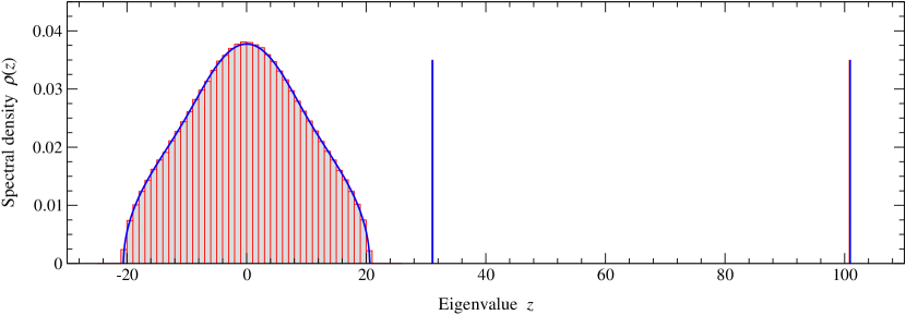
Figure 1: The spectrum of the adjacency matrix for the case of a network with two groups of equal size and $\mathbf{k}_{i}=(\kappa_{i},\pm\theta)$, where $\theta=50$, $\kappa_{i+n/2}=\kappa_{i}$, and $\kappa_{i}$ is either 60 or 120 with equal probability. Blue represents the analytic solution, Eqs. (29) and (39). Red is the numerical diagonalization of the adjacency matrix of a single network with $n=10\,000$ vertices generated from the model with the same parameters. The numerically evaluated positions of the two outlying eigenvalues (the red spikes) agree so well with the analytic values (blue spikes) that the red is mostly obscured behind the blue.

III.3 Spectrum of the adjacency matrix

So far we have derived the spectral density of the centered adjacency matrix $\mathbf{X}=\mathbf{A}-\langle\mathbf{A}\rangle$. We can use the results of these calculations to compute the spectrum of the full adjacency matrix by generalizing the method used in NN13 , as follows.

Using Eq. (5) we can write the adjacency matrix as

$$\mathbf{A}=\mathbf{X}+\langle\mathbf{A}\rangle=\mathbf{X}+\sum_{r=1}^{q}\alpha_{r}\mathbf{u}_{r}\mathbf{u}_{r}^{T}.$$ (34)

Let us first consider the effect of adding just one of the terms in the sum to the centered matrix $\mathbf{X}$, calculating the spectrum of the matrix $\mathbf{X}+\alpha_{1}\mathbf{u}_{1}\mathbf{u}_{1}^{T}$. Let $\mathbf{v}$ be an eigenvector of this matrix with eigenvalue $z$:

$$(\mathbf{X}+\alpha_{1}\mathbf{u}_{1}\mathbf{u}_{1}^{T})\mathbf{v}=z\mathbf{v}.$$ (35)

Rearranging this equation we have $\alpha_{1}\mathbf{u}_{1}\mathbf{u}_{1}^{T}\mathbf{v}=(z-\mathbf{X})\mathbf{v}$ and, multiplying by $\mathbf{u}_{1}^{T}(z-\mathbf{X})^{-1}$, we find

$$\mathbf{u}_{1}^{T}(z-\mathbf{X})^{-1}\mathbf{u}_{1}={1\over\alpha_{1}}.$$ (36)

Note that the vector $\mathbf{v}$ has canceled out of the equation, leaving us with an equation in $z$ alone. The solutions for $z$ of this equation give us the eigenvalues of the matrix $\mathbf{X}+\alpha_{1}\mathbf{u}_{1}\mathbf{u}_{1}^{T}$.

Expanding the vector $\mathbf{u}_{1}$ as a linear combination of the eigenvectors $\mathbf{x}_{i}$ of the matrix $\mathbf{X}$, the equation can also be written in the form

$$\sum_{i=1}^{n}{(\mathbf{x}_{i}^{T}\mathbf{u}_{1})^{2}\over z-\lambda_{i}}={1\over\alpha_{1}},$$ (37)

where $\lambda_{i}$ are the eigenvalues of $\mathbf{X}$. Figure 2 shows a graphical representation of the solution of this equation for the eigenvalues $z$. The left-hand side of the equation, represented by the solid curves, has simple poles at $z=\lambda_{i}$ for all $i$. The right-hand side, represented by the horizontal dashed line, is constant. Where the two intercept, represented by the dots, are the solutions for $z$. From the geometry of the figure we can see that the values of $z$ must fall between consecutive values of $\lambda_{i}$—we say that the $z$’s and $\lambda$’s are interlaced. If we number the eigenvalues $\lambda_{i}$ in order from largest to smallest so that $\lambda_{1}\geq\lambda_{2}\geq\ldots\geq\lambda_{n}$, and similarly for the $n$ solutions $z_{i}$ to Eq. (37), then $z_{1}\geq\lambda_{1}\geq z_{2}\geq\lambda_{2}\geq\ldots\geq z_{n}\geq\lambda_{n}$. In the limit of large system size, as the $\lambda_{i}$ become more and more closely spaced in the spectrum of the matrix, this interlacing places tighter and tighter bounds on the values of $z_{i}$, and asymptotically we have $z_{i}=\lambda_{i}$ and the spectral density of $\mathbf{X}+\alpha_{1}\mathbf{u}_{1}\mathbf{u}_{1}^{T}$ is the same as that of $\mathbf{X}$ alone.

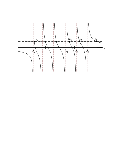
Figure 2: A plot of the left-hand size of Eq. (37) as a function of $z$ has simple poles at $z=\lambda_{i}$ for all $i$. The solutions of the equation fall at the points where the curve crosses the horizontal dashed line representing the value of $1/\alpha_{1}$. From the geometry of the figure we can see that the solutions must lie in between the values of the $\lambda_{i}$, interlacing with them, so that $z_{1}\geq\lambda_{1}\geq z_{2}\geq\ldots\geq z_{n}\geq\lambda_{n}$.

There is one exception, however, in the highest-lying eigenvalue $z_{1}$, which is bounded below by $\lambda_{1}$ but unbounded above, meaning it need not be equal to $\lambda_{1}$ and may lie outside the band of values occupied by the spectrum of the matrix $\mathbf{X}$. To calculate this eigenvalue we observe that, the matrix $\mathbf{X}$ being random, its eigenvectors $\mathbf{x}_{i}$ are also random and hence $\mathbf{x}_{i}^{T}\mathbf{u}_{1}$ is a zero-mean random variable with variance $1/n$. Taking the average of Eq. (37) over the ensemble of networks, the numerator on the left-hand side gives simply a factor of $1/n$ and we have

$${1\over\alpha_{1}}={1\over n}\Biggl{\langle}\sum_{i=1}^{n}{1\over z-\lambda_{i}}\Biggr{\rangle}={1\over n}\bigl{\langle}\operatorname{Tr}(z-\mathbf{X})^{-1}\bigr{\rangle}=g(z).$$ (38)

The solution to this equation gives us the value of $z_{1}$.

This then gives us the complete spectrum for the matrix $\mathbf{X}+\alpha_{1}\mathbf{u}_{1}\mathbf{u}_{1}^{T}$. It consists of a continuous spectral band with spectral density equal to that of the matrix $\mathbf{X}$ alone, which is calculated from Eq. (21), plus a single eigenvalue outside the band whose value is the solution for $z$ of $g(z)=1/\alpha_{1}$.

We could have made the same argument about any single term $\alpha_{r}\mathbf{u}_{r}\mathbf{u}_{r}^{T}$ appearing in Eq. (34) and derived the corresponding result that the continuous spectral band is unchanged from the centered matrix but there can be an outlying eigenvalue $z_{r}$ given by

$$g(z_{r})={1\over\alpha_{r}}.$$ (39)

The calculation of the spectrum of the full adjacency matrix requires that we consider all terms in Eq. (34) simultaneously, but in practice it turns out that it is enough to consider them one by one using Eq. (39). The argument for this is in two parts as follows.

1. We have shown that the spectral density of the continuous band in the spectrum of the matrix $\mathbf{X}+\alpha_{1}\mathbf{u}_{1}\mathbf{u}_{1}^{T}$ is the same as that for the matrix $\mathbf{X}$ alone, and there is one additional outlying eigenvalue, which we denote $z_{1}$. Now we can add another term $\alpha_{2}\mathbf{u}_{2}\mathbf{u}_{2}^{T}$ and repeat our argument for the matrix $\mathbf{X}+\alpha_{1}\mathbf{u}_{1}\mathbf{u}_{1}^{T}+\alpha_{2}\mathbf{u}_{2}\mathbf{u}_{2}^{T}$, finding the equivalent of Eq. (37) to be

   $$\sum_{i=2}^{n}{(\mathbf{x}_{i}^{T}\mathbf{u}_{2})^{2}\over z^{\prime}-z_{i}}+{(\mathbf{x}_{1}^{T}\mathbf{u}_{2})^{2}\over z^{\prime}-z_{1}}={1\over\alpha_{2}},$$ (40)

   where $z^{\prime}$ is the eigenvalue of the new matrix and $z_{i}$ are the solutions of (37). As before, this implies there is an interlacing condition and that the spectral density of the perturbed matrix is the same within the spectral band as that for the unperturbed matrix. We can repeat this argument as often as we like and thus demonstrate that the shape of the spectral band never changes, so long as the number of perturbations (which is also the rank of $\langle\mathbf{A}\rangle$) is small compared to the size of the network, i.e, $q\ll n$.

2. This argument pins down all but the top two eigenvalues of $\mathbf{X}+\alpha_{1}\mathbf{u}_{1}\mathbf{u}_{1}^{T}+\alpha_{2}\mathbf{u}_{2}\mathbf{u}_{2}^{T}$. These two we can calculate by a variant of our previous argument. We average Eq. (40) over the ensemble, noting again that $\langle(\mathbf{x}_{i}^{T}\mathbf{u}_{2})^{2}\rangle=1/n$ and find that

   $${1\over n}\sum_{i=2}^{n}{1\over z^{\prime}-z_{i}}+{1/n\over z^{\prime}-z_{1}}={1\over\alpha_{2}}.$$ (41)

   For large $n$ the first sum is once again equal to the Stieltjes transform $g(z)$ and hence the top two eigenvalues are solutions for $z^{\prime}$ of

   $$g(z^{\prime})+{1/n\over z^{\prime}-z_{1}}={1\over\alpha_{2}}.$$ (42)

   But $g(z)$ and $\alpha_{2}$ are of order 1, while the term $n^{-1}/(z^{\prime}-z_{1})$ is of order $1/n$ and hence can in most circumstances be neglected, giving $g(z^{\prime})=1/\alpha_{2}$, which recovers Eq. (39). The only time this term cannot be neglected is when $z^{\prime}$ is within a distance of order $1/n$ from $z_{1}$, in which case we have a simple pole in the left-hand side of the equation as $z^{\prime}$ approaches $z_{1}$. Thus the left-hand side has the form sketched in Fig. 3, following $g(z)$ closely for most values of $z$, but diverging suddenly when very close to $z_{1}$. Equation (42) then has two solutions, as indicated by the dots in the figure, one given by $g(z)=1/\alpha_{2}$ and one that is asymptotically equal to $z_{1}$, which is the solution of $g(z)=1/\alpha_{1}$.

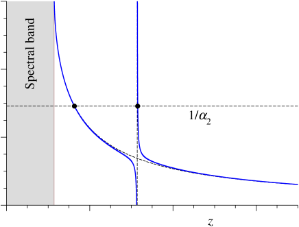
Figure 3: A graphical representation of the solution of Eq. (42). The left-hand size of the equation, represented by the solid blue curve, follows closely the form of the Stieltjes transform $g(z)$, except within a distance of order $1/n$ from $z_{1}$, where it diverges. The horizontal dashed line represents the value $1/\alpha_{2}$ and the solutions to (42), of which there are two, fall at the intersection of this line with the solid curve, as indicated by the dots. One of these solutions coincides closely with $z_{1}$, the other is the solution of $g(z)=1/\alpha_{2}$.

We can repeat this argument as many times as we like to demonstrate that the outlying eigenvalues are just the $q$ solutions of Eq. (39) for each value $r=1\ldots q$. Thus our final solution for the complete spectrum of the adjacency matrix has two parts: a continuous spectral band, given by Eqs. (21) and (22), and $q$ outlying eigenvalues, given by the solutions of Eq. (39), with $g(z)$ given by Eq. (20).

III.4 Examples

Let us return to the examples of Section III.2 and apply the methods above to the calculation of their outlying eigenvalues. Recall that we looked at networks with two communities and chose parameter vectors $\mathbf{k}_{i}=(\kappa_{i},\theta)$ for vertices in the first community and $\mathbf{k}_{i}=(\kappa_{i-n/2},-\theta)$ for those in the second. For such networks the vector function $\mathbf{h}(z)$ reduces to a single scalar function $h_{1}(z)$ that satisfies Eq. (27). At the same time, Eq. (20) tells us that for this model $zg(z)=1+ch_{1}^{2}(z)$ and hence from Eq. (39) the positions of the outlying eigenvalues are solutions of

$$1+ch_{1}^{2}(z)-{z\over\alpha_{r}}=0,$$ (43)

for $r=2\ldots q$. Locating the outliers is thus a matter of solving (27) for $h_{1}$, substituting the result into (43), and then solving for $z$.

Consider, for instance, the choice we made in Section III.2, where there were just two values of $\kappa$, denoted $\kappa_{1}$ and $\kappa_{2}$, with half the vertices in each community taking each value. Then $h_{1}$ obeys the cubic equation (30), which can be solved exactly, and hence we can calculate the position of the outliers. Figure 1 shows the results for the choice $\kappa_{1}=60$, $\kappa_{2}=120$, $\theta=50$, along with numerical results for the same parameter values. As the figure shows, analytic and numerical calculations again agree well—so well, in fact, that the difference between them is quite difficult to make out on the plot.

We also looked in Section III.2 at the simple case where $\kappa=c$ for all vertices, so that they all have the same expected degree, in which case the model becomes equivalent to the standard stochastic block model and the continuous spectral band takes the classic semicircle form of Eq. (33). For this model we have $\alpha_{1}=c$ and $\alpha_{2}=\theta^{2}/c$. Using Eq. (32) for $h_{1}(z)$ and solving (43) for $z$, we then find the top two eigenvalues of the adjacency matrix to be

$$z_{1}=c+1,\qquad z_{2}={\theta^{2}\over c}+{c^{2}\over\theta^{2}},$$ (44)

which agrees with the results given previously for the stochastic block model in Ref. NN12 .

III.5 Detectability of communities

One of the primary uses of network spectra is for the detection of community structure Newman06c ; NN12 . As we have seen, the number of eigenvalues above the edge of the spectral band is equal to the number of communities in the network, and hence the observation of these eigenvalues can be taken as evidence of the presence of communities and their number as an empirical measure of the number of communities. The identity of the communities themselves—which vertices belong to which community—can be deduced, at least approximately, by looking at the elements of the eigenvectors Newman06c .

However, as shown previously in NN12 for the simplest two-community block model, the position of the leading eigenvalues varies as one varies the strength of community structure, and for sufficiently low (but still nonzero) strength an eigenvalue may meet the edge of the spectral band and hence become invisible in the spectrum, meaning it can no longer be used as evidence of the presence of community structure. Moreover, as also shown in NN12 , the elements of the corresponding eigenvector become uncorrelated with group membership at this point, so that any algorithm which identifies communities by examining the eigenvector elements will fail. The point where this happens, at least in the simple two-community model, coincides with the known “detectability threshold” for community structure, at which it is believed all algorithms for community detection must fail RL08 ; DKMZ11a ; HRN12 .

We expect qualitatively similar behavior in the present model as well. Consider the Stieltjes transform $g(z)$ defined in Eq. (15). Inside the spectral band the transform is complex by definition—see from Eq. (18). Above the band it is real and monotonically decreasing in $z$, as we can see by evaluating the trace in the basis in which $\mathbf{X}$ is diagonal:

$$g(z)={1\over n}\sum_{i=1}^{n}{1\over z-\lambda_{i}},$$ (45)

where $\lambda_{i}$ are the eigenvalues of $\mathbf{X}$ as previously. Above the band, where $z>\lambda_{i}$ for all $i$, every term in this sum is monotonically decreasing, and hence so is $g(z)$. This implies via Eq. (39) that larger values of $\alpha_{r}$ give larger eigenvalues and that the largest real value $g_{\textrm{max}}$ of the Stieltjes transform occurs exactly at the band edge. Moreover, as shown in Ref. NN13 , the edge of the band is marked generically by a square-root singularity in the spectral density, which implies that $g_{\textrm{max}}$ is finite—see Fig. 3 for a sketch of the function. Thus when we make the community structure in the network weaker, meaning we decrease the values of the $\alpha_{r}$, we also decrease the outlying eigenvalues of the adjacency matrix and eventually the lowest of those eigenvalues will meet the edge of the band and disappear at the point where $1/\alpha_{r}=g_{\textrm{max}}$. If we continue to weaken the structure, more eigenvalues will disappear, in order—smallest first, then second smallest, and so forth.

Thus we expect there to be a succession of detectability transitions in the network, $q-1$ of them in all, where $q$ again is the number of communities. At the first of these transitions the $q$th largest eigenvalue will meet the band edge and disappear, meaning there will only be $q-1$ outlying eigenvalues left and hence there will be observational evidence of only $q-1$ communities in the network, even if in fact we know there to be $q$. At the next transition the number will decrease further to $q-2$, and so forth. One thus loses the ability to detect community structure in stages, one community at a time. Final evidence of any structure at all disappears at the point where the second largest eigenvalue meets the band edge.

Consider, for instance, the example network from Section III.2 again, in which there are two groups with parameter vectors of the form $(\kappa_{i},\pm\theta)$, where the parameters $\kappa_{i}$ control the expected degrees and $\theta$ controls the strength of the community structure. As before, let us study the case where the $\kappa_{i}$ take just two different values with equal probability, so that $h_{1}$ satisfies the cubic equation (30) (and $h_{2}=0$). Then we can calculate the maximal real value of $g(z)$ as follows.

Like $g(z)$, the function $h_{1}(z)$ is real outside the continuous spectral band but complex inside it, as one can see from Eq. (28). The band edge is thus the point at which the solution of the cubic equation becomes complex, which is given by the zero of the discriminant of the cubic. Take, for example, the case where $\kappa_{1}=\kappa$ and $\kappa_{2}=2\kappa$ for some constant $\kappa$. Then, employing the standard formula, the discriminant of (30) is

$${\kappa^{5}\over 27}\biggl{[}27\biggl{(}{z^{2}\over\kappa}\biggr{)}^{3}-216\biggl{(}{z^{2}\over\kappa}\biggr{)}^{2}+252\biggl{(}{z^{2}\over\kappa}\biggr{)}-512\biggr{]}.$$ (46)

This is zero when, and hence the band edge falls at, $z=\sqrt{x\kappa}$, where $x\simeq 7.058$ is the sole real solution of the cubic equation $27x^{3}-216x^{2}+252x-512=0$. Substituting into Eq. (30), we then find that the value of $h_{1}$ at the band edge is $y/\sqrt{\kappa}$ where $y=0.723$ is the smallest real solution of the cubic equation $2y^{3}-3\sqrt{x}y^{2}+(x+\tfrac{4}{3})y-\sqrt{x}=0$. Then, using Eq. (20) and the fact that the average degree is $c=\frac{3}{2}\kappa$, the value of $g(z)$ at the band edge is

$$g_{\textrm{max}}={2+3y^{2}\over 2\sqrt{x\kappa}}.$$ (47)

In this case there is only one parameter $\alpha_{r}$ with $r\geq 2$, which is $\alpha_{2}=\theta^{2}/c$. Hence there is a single threshold at which we lose the ability to detect communities, falling at

$${c\over\theta^{2}}={2+3y^{2}\over 2\sqrt{x\kappa}},$$ (48)

or

$$\theta=\sqrt{3\sqrt{x\kappa^{3}}\over 2+3y^{2}}\simeq 1.494\kappa^{3/4}.$$ (49)

If $\theta$ is smaller than this value then spectral methods will fail to detect the communities in the network. We have checked this behavior numerically and find indeed that spectral community detection fails at approximately this point.

IV Conclusions

In this paper we have given a prescription for calculating the spectrum of the adjacency matrix of an undirected random network containing both community structure and a nontrivial degree distribution, generated using the model of Ball et al. BKN11 . In the limit of large network size the spectrum consists in general of two parts: (1) a continuous spectral band containing the bulk of the eigenvalues and (2) $q$ outlying eigenvalues above the spectral band, where $q$ is the number of communities in the network. We give expressions for both the shape of the band and the positions of the outlying eigenvalues that are exact in the limit of a large network and large vertex degrees, although their evaluation involves integrals that may not be analytically tractable in practice, in which case we must resort to numerical evaluation. We have compared the spectra calculated using our method with direct numerical diagonalizations and find the agreement to be excellent. Based on our results we also argue that there should be a series of $q-1$ “detectability transitions” as the community structure gets weaker, at which one’s ability to detect communities becomes successively impaired. The positions of these transitions correspond to the points at which the outlying eigenvalues meet the edge of the spectral band and disappear. With the disappearance of the second-largest eigenvalue in this manner, all trace of the community structure vanishes from the spectrum and the network is indistinguishable from an unstructured random graph.

- (1) M. E. J. Newman, The structure and function of complex networks. SIAM Review 45, 167–256 (2003).
- (2) S. Boccaletti, V. Latora, Y. Moreno, M. Chavez, and D.-U. Hwang, Complex networks: Structure and dynamics. Physics Reports 424, 175–308 (2006).
- (3) M. Fiedler, Algebraic connectivity of graphs. Czech. Math. J. 23, 298–305 (1973).
- (4) A. Pothen, H. Simon, and K.-P. Liou, Partitioning sparse matrices with eigenvectors of graphs. SIAM J. Matrix Anal. Appl. 11, 430–452 (1990).
- (5) M. E. J. Newman, Finding community structure in networks using the eigenvectors of matrices. Phys. Rev. E 74, 036104 (2006).
- (6) P. F. Bonacich, Power and centrality: A family of measures. Am. J. Sociol. 92, 1170–1182 (1987).
- (7) I. J. Farkas, I. Derényi, A.-L. Barabási, and T. Vicsek, Spectra of “real-world” graphs: Beyond the semicircle law. Phys. Rev. E 64, 026704 (2001).
- (8) K.-I. Goh, B. Kahng, and D. Kim, Spectra and eigenvectors of scale-free networks. Phys. Rev. E 64, 051903 (2001).
- (9) F. Chung, L. Lu, and V. Vu, Spectra of random graphs with given expected degrees. Proc. Natl. Acad. Sci. USA 100, 6313–6318 (2003).
- (10) S. N. Dorogovtsev, A. V. Goltsev, J. F. F. Mendes, and A. N. Samukhin, Spectra of complex networks. Phys. Rev. E 68, 046109 (2003).
- (11) R. Kühn, Spectra of sparse random matrices. J. Phys. A 41, 295002 (2008).
- (12) S. Chauhan, M. Girvan, and E. Ott, Spectral properties of networks with community structure. Phys. Rev. E 80, 056114 (2009).
- (13) R. R. Nadakuditi and M. E. J. Newman, Graph spectra and the detectability of community structure in networks. Phys. Rev. Lett. 108, 188701 (2012).
- (14) R. R. Nadakuditi and M. E. J. Newman, Spectra of random graphs with arbitrary expected degrees. Phys. Rev. E 87, 012803 (2013).
- (15) P. W. Holland, K. B. Laskey, and S. Leinhardt, Stochastic blockmodels: Some first steps. Social Networks 5, 109–137 (1983).
- (16) A. Condon and R. M. Karp, Algorithms for graph partitioning on the planted partition model. Random Structures and Algorithms 18, 116–140 (2001).
- (17) J. Reichardt and M. Leone, (Un)detectable cluster structure in sparse networks. Phys. Rev. Lett. 101, 078701 (2008).
- (18) A. Decelle, F. Krzakala, C. Moore, and L. Zdeborová, Inference and phase transitions in the detection of modules in sparse networks. Phys. Rev. Lett. 107, 065701 (2011).
- (19) D. Hu, P. Ronhovde, and Z. Nussinov, Phase transitions in random Potts systems and the community detection problem: Spin-glass type and dynamic perspectives. Phil. Mag. 92, 406–445 (2012).
- (20) M. Molloy and B. Reed, A critical point for random graphs with a given degree sequence. Random Structures and Algorithms 6, 161–179 (1995).
- (21) M. E. J. Newman, S. H. Strogatz, and D. J. Watts, Random graphs with arbitrary degree distributions and their applications. Phys. Rev. E 64, 026118 (2001).
- (22) F. Chung and L. Lu, The average distances in random graphs with given expected degrees. Proc. Natl. Acad. Sci. USA 99, 15879–15882 (2002).
- (23) B. Ball, B. Karrer, and M. E. J. Newman, An efficient and principled method for detecting communities in networks. Phys. Rev. E 84, 036103 (2011).
- (24) Z. Bai and J. W. Silverstein, Spectral analysis of large dimensional random matrices. Springer, Berlin, 2nd edition (2010).
- (25) S. Molchanov, L. Pastur, and A. Khorunzhii, Limiting eigenvalue distribution for band random matrices. Theoretical and Mathematical Physics 90, 108–118 (1992).
- (26) D. Shlyakhtenko, Random Gaussian band matrices and freeness with amalgamation. International Mathematics Research Notices 1996, 1013–1025 (1996).
- (27) G. Anderson and O. Zeitouni, A CLT for a band matrix model. Probability Theory and Related Fields 134, 283–338 (2006).
- (28) G. Casati and V. Girko, Wigner’s semicircle law for band random matrices. Random Operators and Stochastic Equations 1, 15–22 (2009).
- (29) Z. Bai and L. Zhang, The limiting spectral distribution of the product of the Wigner matrix and a nonnegative definite matrix. Journal of Multivariate Analysis 101, 1927–1949 (2010).