Exact solution of rectangular Ising lattice in a uniform external field

Abstract

A method is proposed for exactly calculating the partition function of a rectangular Ising lattice with the presence of a uniform external field. This approach is based on the method of the transfer matrix developed about seventy years ago for the rectangular Ising model in the absence of external field. The basis for the vector space is chosen as the eigenvectors of the diagonal part of the transfer matrix. The matrix elements for the non-diagonal part can be calculated very easily. Then the partition function and thermodynamical quantities can be evaluated. The limit of infinite lattice is discussed.

PACS number(s): 05.50.+q, 64.60.an, 75.30.Kz

The study of various phase transitions has been an extremely important research subject in many fields, because phase transitions are common in physics and familiar in everyday life, as liquid water freezes at zero census degree, the formation of binary alloys and the phenomenon of ferromagnetism. In spite of their familiarity, phase transitions are not well understood. The Ising model Ising , which was initially proposed to explain how short-range interactions give rise to long-range, correlative behavior, and to predict in some sense the potential for a phase transition or spontaneous magnetization, has been one of the most important models in investigating phenomena involving a phase transition. There is no other local model that incorporates a phase transition that can be analyzed at anything like the resolution that is possible for the Ising model Palmer . The Ising model has attracted enormous interest and also been applied to problems in chemistry, molecular biology, and other areas where “cooperative” behavior of large systems is studied, and more than thousand research papers published on properties of systems described by the model.

The one-dimensional Ising model model, which was suggested by Ernst Ising in the early 1920s, can be solved easily but does not exhibit a phase transition at any finite temperature. The interest in the model was revived when in 1936 R. Peierls argued peierls that the two-dimensional Ising model should have a phase transition. The transition point was located by Kramers and Wannier in 1941 kramers . The exact solution for the partition function of the rectangular Ising model was obtained in 1944 by L. Onsager onsager by using the transfer matrix method introduced in montr ; kramers , when there is no external field interacting on the lattice system. In 1949 B. Kaufman simplified Onsager’s calculations kaufman . Since then, many different methods have been developed for studying the thermodynamical properties of the Ising model in the absence of external field. For a recent review, one can read Palmer ; hystad . Up to now, however, the two-dimensional Ising model in the presence of a uniform external field has not been solved exactly, and Monte Carlo simulation is the only way to study the properties of the Ising lattice under the influence of external field. Such simulation is powerful only for lattices of small sizes because of the limitation of computer memory and takes a long time for computing physical quantities to a high accuracy. Because of the extremely wide applications of the model, finding an exact solution of the in-field model is very important and may bring us deeper understanding of the model and the phenomenon of magnetization and order-disorder transitions.

In this paper, based on the results of onsager and kaufman , a method is proposed for calculating exactly the partition function of the rectangular Ising model in the presence of a uniform external field. The transfer matrix for an $N\times M$ lattice is represented by a $2^{N}\times 2^{N}$ matrix. The partition function of the system can be obtained by calculating the maximum eigenvalue of the matrix. No approximation is made in the process, thus the solution obtained is exact for $M$ larger enough.

For an $N\times M$ rectangular Ising lattice in a uniform external field, the Hamiltonian of the system can be written as

$$\varepsilon=-\sum_{i,j}(J_{1}\sigma_{i,j}\sigma_{i+1,j}+J_{2}\sigma_{i,j}\sigma_{i,j+1})-H\sum_{i,j}\sigma_{i,j}\ ,$$ (1)

with the coupling constants between spins on the nearest neighboring sites $J_{1}>0,J_{2}>0$ and a uniform external magnetic field $H>0$. In the above equation, any $\sigma_{i,j}$ can take only two values, $\pm 1$. The partition function can be expressed in terms of the transfer matrices as, in a way similar to that used in onsager ,

$$Z=(\exp K_{2})^{MN}{\rm Tr}(V_{1}V_{2}V_{3})^{M}\ ,$$ (2)

where

$$V_{1} = \prod_{j=1}^{N}(1+tC_{j})\ ,\ \ t=\exp(-2K_{2})\ ,$$ (3)

$$V_{2} = \prod_{j=1}^{N}\exp(K_{1}\sigma_{j}\sigma_{j+1})\ ,$$ (4)

$$V_{3} = \prod_{j=1}^{N}\exp(h\sigma_{j})\ .$$ (5)

In the above expressions, $h=\beta H,K_{i}=\beta J_{i}$ for $i=1,2$. Here $\beta=kT$ and $\sigma_{j}=\left(\begin{array}[]{cc}1&0\\ 0&-1\\ \end{array}\right)$ and $C_{j}=\left(\begin{array}[]{cc}0&1\\ 1&0\\ \end{array}\right)$ are operators acting on the spin of site $j$ in a row. When acting on a state function, the operator $\sigma_{j}$ gives us the spin ($\pm 1$) for the $j$-th site in a row, but $C_{j}$ will reverse the spin of that site. The operators $C_{j}$ and $\sigma_{j}$ satisfy the following quaternion algebra relations

$$\sigma_{i}\sigma_{j} = \sigma_{j}\sigma_{i},\ \ C_{i}C_{j}=C_{j}C_{i},$$

$$C_{i}\sigma_{j} = (-1)^{\delta_{i,j}}\sigma_{j}C_{i}\ ,\ \ C_{j}^{2}=\sigma_{j}^{2}=1\ .$$

The partition function can be written in terms of the eigenvalues $\lambda_{i}$ of $V_{1}V_{2}V_{3}$ as $Z=(\exp(K_{2}))^{MN}\sum_{i=1}^{N}\lambda_{i}^{M}$. When the lattice size $M$ is large enough, only the maximum eigenvalue $\lambda$ is needed for calculating the partition function. In solving the eigenvalue problem, one can use a “wrap-around” model, therefore, $\sigma_{N+1}=\sigma_{1}$. In onsager ; kaufman , a chiral operator $U=\prod_{j=1}^{n}C_{j}$ was defined and the matrix $V_{1}^{1/2}V_{2}V_{1}^{1/2}$ can be decomposed as a direct sum of two parts corresponding to $U=1$ and $U=-1$, respectively. Denote those eigenvectors of $V_{1}^{1/2}V_{2}V_{1}^{1/2}$ corresponding to $U=1$ by $\Psi^{+}$, those corresponding to $U=-1$ by $\Psi^{-}$. The former is even under operation of $U$, and the latter is odd. Because $V_{1}^{1/2}V_{2}V_{1}^{1/2}$ is a Hermitian operator, the eigenvectors $\Psi^{+}$ and $\Psi^{-}$ form a complete orthogonal basis for the vector space in question. Naively, a natural extension of the method to the case with a uniform external field would be to calculate matrix elements of $V_{3}$ in the vector space spanned by $\Psi^{+}$ and $\Psi^{-}$. Because the operator $V_{3}$ does not commute with $U$, the acting of $V_{3}$ will cause a mixing between states of $\Psi^{+}$ and $\Psi^{-}$. When the external field is weak, standard perturbation theory can be used to obtain the partition function and the spontaneous magnetization cnyang . For this case, the only mixing needed for consideration is that between the two states $\Psi^{+}$ and $\Psi^{-}$ corresponding to maximum eigenvalues. For the general case when the external field is not weak, mixing among all states is possible and needed for solving the eigenvalue problem. Then one has to work with a dense $2^{N}\times 2^{N}$ matrix, thus analytical solution to the problem may be impossible for finite $M$ and $N$. It will be shown in this paper that an exact solution can still be obtained.

To get the matrix elements for $V_{1}V_{2}V_{3}$, the eigenvectors $\Psi^{+}$ and $\Psi^{-}$ for $V_{1}^{1/2}V_{2}V_{1}^{1/2}$ are not a good choice as the basis, because those eigenvectors cannot be used easily in calculating the spin matrix elements. If one wishes to calculate the spin matrix of only one site, the site at the center of lattice for example, the method in bugrij can be used. We need, however, the spin matrix elements for all spins in a row, and the method used in bugrij does not work. Alternatively, to set up a basis, one can first solve the eigenvalue problem for operator $V_{2}V_{3}$. This is a simple problem, because that operator is diagonal in the meaning that it depends only on the spin configuration of sites in a row. Thus this problem is like a one-dimensional Ising model. One can identify an eigenvector of $V_{2}V_{3}$ by a set of sites with spin down, such as $|\emptyset\rangle$ for the state with no spin down, $|2\rangle$ for the state with only one (the second site) spin down, etc. If there are $n$ sites with spin down, there are $N!/n!(N-n)!$ possible ways to distribute those sites in a row. Therefore, we have in total $2^{N}$ eigenvectors for the operator $V_{2}V_{3}$. It is apparent that the set of such eigenvectors forms a complete orthogonal basis for the problem involved. The eigenvalue of $V_{2}V_{3}$ corresponding to any one of those states can be easily calculated, since it is determined only by the number of sites with spin down ($N_{-}$) and the number of nearest neighboring down-down spin pairs ($N_{--}$). These two numbers can be easily counted when the sites with spin down is fixed. Then the next task is to calculate the matrix elements of $V_{1}$ on the basis. A crucial observation is that an eigenvector of $V_{2}V_{3}$ with $n$ sites spin down, $|I_{n}\rangle$ with $I_{n}$ the set of sites with spin down, can be expressed as

$$|I_{n}\rangle=\prod_{j\in I_{n}}C_{j}|\emptyset\rangle\ .$$ (7)

Because $C_{i}^{2}=1$ for any $i$, the action of $C_{i}$ on $|I_{n}\rangle$ may increase the number of spin down sites from $n$ to $n+1$ if the site $i$ is not included in $I_{n}$. Otherwise, $n$ will be decreased to $n-1$. Therefore the operator $C_{i}$ can be an annihilation or a creation operator, depending on whether $i$ is in the set $I_{n}$ or not. This observation makes the calculation of matrix elements for $V_{1}$ extremely easy. To obtain the matrix elements for $V_{1}$, one first expands $V_{1}$ as

$$V_{1}=\sum_{m=0}^{N}t^{m}\sum_{I_{m}}\prod_{j\in I_{m}}C_{j}\ ,$$ (8)

where $I_{m}$ is a set of $m$ different integers from 1 to $N$, and the summation over $I_{m}$ runs for all possible different sets. Then a matrix element of $V_{1}$ between two states $|I_{n}\rangle$ and $|I_{l}\rangle$, $\langle T_{l}|V_{1}|I_{n}\rangle$, is

$$V_{1}(n,l)=\sum_{m=0}^{N}t^{m}\sum_{I_{m}}\langle\emptyset|\prod_{i\in I_{l}}C_{i}\prod_{j\in I_{m}}C_{j}\prod_{k\in I_{n}}C_{k}|\emptyset\rangle\ .$$ (9)

Considering that the operator $C_{j}$ can be an annihilation or creation operator in different situations, only one term in the above expression has nonzero value. That term has a special property that in the set $I=I_{l}\bigcup I_{m}\bigcup I_{n}$, each site involved appears exactly twice. In other words, the nonzero term in the above equation has $m$ equal to the number of different sites in sets $I_{l}$ and $I_{n}$, because any site can be in $I_{l}$ and/or $I_{n}$ at most once. Therefore, $V_{1}(n,l)=t^{m}=V_{1}(l,n)$ with $m$ uniquely determined by the difference of sets $I_{n}$ and $I_{l}$, $m=n+l-2({\rm number\ of\ common\ sites})$. So $V_{1}(n,n)=1$ for any $n$. Then the eigenvalue problem for the rectangular Ising model in a unifrom external field

$$(V_{2}V_{3})^{1/2}V_{1}(V_{2}V_{3})^{1/2}\Psi=\lambda\Psi\ ,$$ (10)

can be rewritten as

$$BA=\lambda A\ ,$$ (11)

where all the elements of $B$ are positive

$$B_{l,n}=B_{n,l}=\mu_{l}t^{m}\mu_{n}\ ,$$ (12)

with $\mu_{l}=\exp(K_{1}(N-4N_{-}+4*N_{--})/2+h(N-2N_{-})/2)$ the eigenvalue of $(V_{2}V_{3})^{1/2}$ corresponding to $|I_{l}\rangle$. The vector $A$ in Eq. (11) is for the expanding coefficients of $\Psi$ on the basis of $I_{n}$. There are effective ways for calculating the eigenvalue $\lambda$ with maximum magnitude for such a symmetric matrix. From $\lambda$ all thermodynamical quantities can be calculated.

In this paper, we only consider the case with $J_{1}=J_{2}=J$, thus $K_{1}=K_{2}=K$. We first investigate the temperature dependence of the mean spin per site $\langle\sigma\rangle=\overline{\sum_{ij}\sigma_{ij}}/MN$ for an arbitrary chosen field $H=0.1J$. It is obvious that

$$\langle\sigma\rangle=\frac{\partial\ln Z}{\partial h}/MN=\frac{\partial\ln\lambda}{\partial h}/N\ .$$ (13)

Since the temperature $T$ appears in the problem always together with $J$ and $H$, one can get the $T$ dependence of $\langle\sigma\rangle$ from its $K=\beta J$ dependence, which is shown in Fig. 1. With the decrease of temperature or increase of $K$ from 0 to 1, $\langle\sigma\rangle$ increases smoothly from 0 to 1, very quickly in the small $K$ region and saturating slowly in the low temperature (large $K$) region. For comparison with the spontaneous magnetization for the field free situation mccoy , the $K$ dependence of $\langle\sigma\rangle$ at $h=0$ for an infinite rectangular Ising lattice is drawn also in Fig.1. At high temperature (or small $K$), the external field makes $\langle\sigma\rangle$ larger than zero while the spontaneous magnetization is nonzero only for $T<T_{C}$ or $K>K_{C}$. When the temperature is low enough, the difference in $\langle\sigma\rangle$ for the two cases is very small, because almost all spins have been aligned to the direction of the external field without external field. It is obvious in the figure that the presence of external field makes the behavior of $\langle\sigma\rangle$ analytic, very different from that at $H=0$ .

Figure 1: The mean magnetization per site $\langle\sigma\rangle$ as a function of parameter $K=\beta J$ for fixed $H=0.1J$. The dashed curve for the case $h=0$ is drawn according to Eq. (4.9) on page 245 of Ref. mccoy .

We are more interested in the dependence of quantities on the external field $H$. Therefore, one can study the $H$ dependences of $\langle\sigma\rangle$ and the mean energy per site. For this purpose, we fix the coupling $J_{1}=J_{2}=k$ as an example, and investigate the dependence of $\langle\sigma\rangle$ on $H/k$ for a few temperatures T=1.0, 2.0, 4.0 and 6.0. The results are shown in Fig. 2. At low temperature $T=1.0$, which is well below the critical temperature for the case with $H=0$, $\langle\sigma\rangle$ is almost 1 even for very weak external field. With the increase of $T$, $\langle\sigma\rangle$ becomes smaller in low $H$ region and increases with $H$.

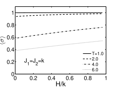
Figure 2: The mean magnetization per site $\langle\sigma\rangle$ as a function of $H/k$ for fixed $J_{1}=J_{2}=k$ at four temperatures.

One can get the mean energy $E$ per site from

$$-\beta E=\left(K\frac{\partial\ln Z}{\partial K}+h\frac{\partial\ln Z}{\partial h}\right)/(MN)\ .$$ (14)

The numerical results for $-\beta E$ are shown in Fig. 3.

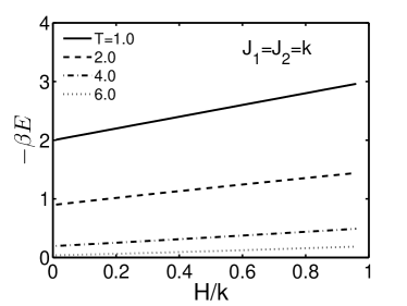
Figure 3: The product of $-\beta$ and the mean energy per site $E$ as a function of $H/k$ for fixed coupling $J_{1}=J_{2}=k$ at four temperatures as in Fig. 2.

At the four temperatures as in Fig.2, the product $-\beta E$ depends approximately linearly on the external field $H$ in the region shown. This can be understood in combination with the $K$ dependence of $\langle\sigma\rangle$ in Fig.1. Even at $T=4.0,K=\beta J=0.25$, $\langle\sigma\rangle$ is about 0.7. Thus the increase of $-\beta E$ from the spin-spin interaction is very small with the increase of $H$. The increase of $-\beta E$ with $H$ comes mainly from the field-spin interaction term which is proportional to the strength $H$ of the external field. At low temperature, the mean energy is not zero at zero external field, because of the spontaneous magnetization. At $H=0$, the lower the temperature, the more the aligned spins, the lower the energy.

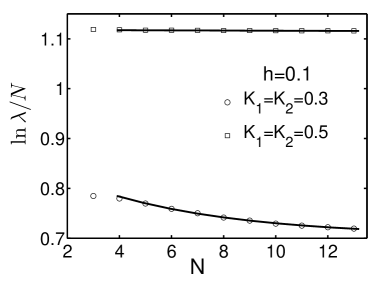
Figure 4: The lattice size $N$ dependence of the maximum eigenvalue $\lambda$ at two cases with different values of $K=0.5$ and 0.3 but with fixed external field $h=0.1$. The solid curve is from fitting the results to Eq. (15).

The method described in this paper can be used for finite $N$, whereas the value of $M$ can be arbitrarily large. The matrix involved in calculating the maximum eigenvalue is $2^{N}\times 2^{N}$, thus its dimension increases very fast with $N$. For real applications, one needs to study the thermodynamical limit, $N\to\infty$ and $M\to\infty$. The $N$ dependence of the maximum eigenvalue $\lambda$ is shown in Fig. 4, for two cases, one with $K_{1}=K_{2}=0.5$, the other with $K_{1}=K_{2}=0.3$, while the external field is fixed at $h=0.1$. For larger $K_{1}=K_{2}$, $\ln\lambda/N$ is larger. For the case with higher $K_{1}=K_{2}$, the lattice size $N$ dependence of $\ln\lambda/N$ is weaker. One can see that, with the increase of lattice size $N$, $\ln\lambda/N$ decreases and approaches its saturation value quickly. In fact, points shown in Fig.4 for the two cases can be well described by

$$\ln\lambda/N=a+b\exp(-cN)\ ,$$ (15)

with the saturation value $a=1.106$ for the case with $K_{1}=K_{2}=0.5$ and 0.704 for the other case. The fitted value of the parameter $c$ equals to 0.187 for the smaller $K_{1}=K_{2}$ case, while it is $5.69\times 10^{-5}$ for the other case. Similarly, the lattice size dependence and the infinite $N$ limit for thermodynamical quantities can be obtained.

The method developed in this paper can be extended to situations much more complicated. When $J_{2}$ depends on the position of column, $J_{2}$ in Eq. (1) must be replaced by $J_{2j}$. For this case, the only modifications are replacements of $\exp(NK_{2})$ in Eq. (2) by $\prod_{j}\exp(K_{2j})$ and $t^{m}$ in Eq. (12) by $\prod_{j}t_{j}$. When the coupling $J_{1}$ depends on the position $j$, the method in this paper can also be used with a modification $K_{1}\to K_{1j}$. In this case, the eigenvalues $\mu_{l}$ and $\mu_{n}$ in Eq. (12) cannot be expressed simply in terms of $N_{-}$ and $N_{--}$ only, but depend on the partition of the spin down-down pairs to a row. If the external field is fixed but not uniform, similar extension can also be made.

In summary, we proposed a method for exactly calculating the partition function of the rectangular Ising model with the presence of a uniform external field. With suitably chosen basis, the elements of the transfer matrix and the maximum eigenvalue can be evaluated without any approximation. The temperature and field strength dependence of the mean magnetization and mean energy per site are presented. Though this method can be used only for a lattice with finite size in one direction, the infinite limit can be obtained from the lattice size dependence of the thermodynamical quantities. Applications of the method to much more complicated situations are straightforward.

This work was supported in part by the National Natural Science Foundation of China under Grant Nos. 11075061 and 11221504, by the Ministry of Education of China under Grant No. 306022 , and by the Programme of Introducing Talents of Discipline to Universities under Grant No. B08033.

References

- (1) E. Ising, Zeits. f. Physik, 31, 253 (1925).
- (2) J. Palmer, Prog. Math. Phys. 49 (Birkhäuser Boston, 2007).
- (3) R. Peierlsm Proc. Camb. Phil. SOc. 32, 477 (1936).
- (4) H.A. Kramers and G.H. Wannier, Phys. Rev. 60, 263 (1941).
- (5) L. Onsager, Phys. Rev. 65, 117 (1944).
- (6) E. Montroll, J. Chen. Phys. 9, 706 (1941).
- (7) B. Kaufman, Phys. Rev. 76, 1232 (1949).
- (8) G. Hystad, J. Math. Phys. 52, 013302 (2011).
- (9) C.N. Yang, Phys. Rev. 85, 808 (1952).
- (10) A.I. Bugrij and O. Lisovyy, Phys. Lett. A 319, 390 (2003); J. Palmer and G. Hystad, J. Math. Phys. 51, 123301 (2010).
- (11) B.M. Mccoy and T.T. Wu, The two-dimensional Ising model, Harvard University Press, Canbridge, Massachusetts, 1973.